The Radial Orbit Instability in Collisionless N-Body Simulations

Abstract

Using a suite of self-gravitating, collisionless $N$-body models, we systematically explore a parameter space relevant to the onset and behavior of the radial orbit instability (ROI), whose strength is measured by the systemic axis ratios of the models. We show that a combination of two initial conditions, namely the velocity anisotropy and the virial ratio, determines whether a system will undergo ROI and exactly how triaxial the system will become. A third initial condition, the radial shape of the density profile, plays a smaller, but noticeable role. Regarding the dynamical development of the ROI, the instability a) begins after systems collapse to their most compact configuration and b) evolves fastest when a majority of the particles have radially anisotropic orbits while there is a lack of centrally-concentrated isotropic orbits. We argue that this is further evidence that self-reinforcing torques are the key to the onset of the ROI. Our findings support the idea that a separate orbit instability plays a role in halting the ROI.

1. Introduction

$N$-body simulations of self-gravitating, collisionless systems of massive particles have become a standard tool used to investigate the behavior of galactic systems. Such particle aggregations can represent the visible, stellar components of galaxies as well as the dark matter that is hypothesized to surround individual galaxies (halos). Since the dark matter halos of galaxies are thought to contain the majority of the mass in a galactic system, the simplest approximation to modeling a real galaxy is to ignore the stars and focus on the dark matter.

This approach has led to cosmological simulations that produce cosmic webs of dark matter, where hierarchical merging creates sub-galactic, galactic, and cluster sized systems. More sophisticated models (like the Millenium Simulation, Springel et al., 2005) also include gas and stars, but the dark matter remains the dominant gravitational component. Simulations like these have found a number of interesting properties of dark matter systems. The density profiles of dark matter halos tend to have shapes described by a simple relation (e.g., Navarro et al., 2004). Generically, density increases with decreasing radius, but the increase is larger near the edges of systems. The overall shape of the density profiles appears to be a robust outcome of dark matter halo evolution (Le Delliou & Henriksen, 2003; Lu et al., 2006; Gonzalez-Casado et al., 2007). However, the inclusion of gaseous baryonic material can impact the innermost regions of dark matter halos (Kazantzidis, Zentner, & Kravtsov, 2006), possibly playing an important role in halo evolution.

Our overall goal is to better understand the physics involved in the evolution of dark matter halos. Such understanding should explain, for example, the shapes of halo density profiles and why the coarse-grained phase-space density is single power-law in radius (Taylor & Navarro, 2001; Barnes et al., 2007). In this work, we focus on models that involve, to some degree, the well-discussed radial orbit instability (ROI) (for example, Polyachenko & Shukhman, 1981; van Albada, 1982; Merritt & Aguilar, 1985; Palmer & Papaloizou, 1987; Katz, 1991; Saha, 1991; Cincotta, Nunez, & Muzzio, 1996; Theis & Spurzem, 1999; Huss, Jain, & Steinmetz, 1999; Barnes et al., 2005; MacMillan, Widrow, & Henriksen, 2006; Boily & Athanassoula, 2006; Bellovary et al., 2008). To this end, we have constructed a set of $N$-body models with a variety of defining characteristics to represent dark matter halos. These models have been evolved in time, and the evolutions have been analyzed to find common trends in behavior.

The ROI can be briefly summarized as follows. Initally spherical $N$-body systems made up of particles that have predominantly radial motions do not remain spherical. In general, the overall shapes of these systems become prolate spheroidal or triaxial (but on time scales of order the relaxation time, they can become more spherical again, see Theis & Spurzem, 1999). The instability appears in models with and without Hubble expansion. As this instability can drive changes in the density and velocity distributions in dark matter systems, we are interested in furthering the description and understanding of its mechanisms.

We will present relationships between initial conditions of $N$-body models and the behavior of the ROI. In particular, we show that neither global measures of velocity anisotropy nor virial ratio alone can be used to predict the onset of the ROI. Instead, we find that combining these measures provides a determination of the end result of the ROI, specifically the overall shape of the system. We also argue that the results of our simulations support the idea that another orbit instability, detailed by Adams et al. (2007), plays an important role in halting the ROI. However, we point out that our simulations cannot speak to any possible role gas could play in stopping the ROI.

As a first step in gathering information about the physics of collisionless, self-gravitating systems, we investigate models that do not include Hubble expansion. As we will discuss, these non-cosmological systems contain complexities that would be compounded by the inclusion of initial radial expansion. Section 2 begins with an explanation of our model creation and evolution methods. Our analysis routines and testing criteria are also described in this section. The crux of this work begins with § 3, a discussion of the global behavior of the ROI in our models. Section 4 deals with our observations of the onset and early development of the ROI. Executive summaries of these topics can be found in Sections 3.3, 4.1.3, and 4.2.4. A synopsis of this work and our conclusions are presented in § 5.

2. Methods & Testing

2.1. Initial Conditions

We create $N$-body systems with three different initial density profiles; $\rho=\rho_{0}$ (constant), $\rho\propto r^{-1}$ (cuspy), and $\rho\propto e^{-r^{2}}$ (Gaussian). Particles are distributed randomly within a sphere of radius $R=1$ according to the density distribution so that the total mass $M=1$. Both $R$ and $M$ are discussed in dimensionless code units where $G=1$; fixing a physical value of $M$ and $R$ would allow us to also transform any other quantities to physical units. The cuspy and Gaussian profiles involve scalelengths; the density at the scalelength is half its central value for the cuspy profile and $e^{-1}$ times its central value for the Gaussian profile. The cuspy scalelength is $10^{-3}$ and the Gaussian scalelength is $1/\sqrt{5}$. The density profile of a cuspy system is shown in Figure 1a. For most of our simulations, the particles have equal masses, but we have also created models with particles of different mass (see § 2.3). For these multi-mass models, the fractions of particles with each mass is determined so that the total mass of the system remains $M=1$.

With the initial positions of the particles fixed, we calculate the potential energy of a system and adopt a value for the initial virial ratio $Q_{0}\equiv T/|W|$ to calculate a scale speed that is used to assign individual particle velocities. The virial ratio changes during the evolution of the systems, and we denote its value at times after $t=0$ simply as $Q$. Velocities are assigned to particles based on an assumed radial velocity anisotropy profile, where $\beta=1-\sigma^{2}_{\rm tan}/2\sigma^{2}_{\rm rad}$ is the velocity anisotropy and $\sigma$ denotes velocity dispersion. We utilize the anisotropy profile discussed in Barnes et al. (2007),

$$\beta(r)=\frac{1}{2}(\beta_{\rm high}-\beta_{\rm low})[1+\tanh{(m\log{r/r_{a}})}]+\beta_{\rm low},$$ (1)

where $\beta_{\rm low}$ is the anisotropy value at $r=0$, $\beta_{\rm high}$ is the value at large $r$, $m$ controls the transition between these values, and $r_{a}$ is the anisotropy radius, at which $\beta=0.5$. The flexibility of this relation allows us to easily create completely isotropic models ($\beta=0$), completely radially anisotropic models ($\beta=1$), or systems with intermediate levels of radial anisotropy. With fixed values of $\beta_{\rm low}$ and $\beta_{\rm high}$, the amount of anisotropy is controlled mainly by the value of $r_{a}$, but the value of the slope $m$ also contributes. For the work discussed here, we have fixed the slope value $m=7$ to provide a relatively rapid change between $\beta_{\rm low}$ and $\beta_{\rm high}$. Note that a given anisotropy profile will provide different amounts of mass with radially anisotropic velocities depending on the density profile. An example $\beta(r)$ with $\beta_{\rm low}=0$, $\beta_{\rm high}=1$, and $r_{a}=0.5$ is plotted in Figure 1b.

For a chosen anisotropy profile, we proceed to assign individual velocities to particles. A particle’s speed can be taken from a distribution about the scale speed. In isotropic regions, particles have velocity directions that uniformly cover $4\pi$ steradians. Radial anisotropy is guaranteed by limiting the velocity vector to lie within cones centered on a particle with axes along the radial direction (one cone opens towards the center, the other opens outward). The opening angle of the cone correlates to the desired value of $\beta$. For small $\beta$, the angle is close to $\pi$; when $\beta\approx 1$, the angle is nearly 0. The velocity vector for a specific particle is chosen randomly within the allowed range of directions. Since the vector has definite limits placed on its direction, we refer to this as the ‘hard-edge’ setup. Panels c and d of Figure 1 show the average component velocities and dispersions, respectively, for a model with the same anisotropy parameters as above and $Q_{0}=0.5$. The average component velocities for all shells in all models are initially zero.

Of course, this is not the only route to initially anisotropic systems. We have also created models with initial conditions that contain combinations of isotropic and radially anisotropic orbits at all radii, in contrast to the ‘hard-edge’ setup. The evolutions of these ‘soft-edge’ models is very similar to those using the ‘hard-edge’ setup. All initially anisotropic models subsequently discussed use the ‘hard-edge’ setup.

2.2. Evolution & Analysis

We have used the direct $N$-body integration code NBODY2 and the treecode Gadget-2 to evolve our ensembles of particles. Readers interested in the details of NBODY2 and Gadget-2 algorithms are encouraged to examine Aarseth (2001) and Springel (2005), respectively. Any two particles $i$ and $j$ interact through softened forces of the form,

$$\vec{F}_{ij}=-G\frac{m_{i}m_{j}}{(r_{ij}^{2}+\epsilon^{2})^{3/2}}(\vec{r}_{i}-\vec{r}_{j}),$$ (2)

where $r_{ij}$ is the distance between the particles and $\epsilon$ is the softening length. NBODY2 allows particle-particle merging, but we do not implement that option in our models. The time interval in these models is the crossing time determined by the initial density profile. A typical run evolves the system for approximately 20 inital crossing times $\>t_{\rm cross}$. The actual length of an evolution depends on the strength of the collapse, with stronger collapses running for fewer crossing times as close particle encounters decrease timestep sizes. However, all simulations have been run long enough for the system to come to virial equilibrium, and most have reached mechanical equilibrium throughout. Some models have an outer region containing $\approx$ 5% of the total mass that continues to expand throughout the simulations. NBODY2 includes a routine for removing particles that become unbound from the system, however Gadget-2 does not. The direct nature of NBODY2 limits the particle numbers that we can reasonably investigate (in this work $N=10^{4}$). As a treecode, Gadget-2 allows us to evolve models with an order of magnitude more particles ($N=10^{5}$) in roughly the same amount of time. Aside from the ability to remove escapers with NBODY2, the biggest difference between the two codes is that energy conservation is much better with NBODY2 (but adequate with Gadget-2).

Output from both codes occurs at fixed intervals determined by the initial crossing time of the system $\>t_{\rm cross}$. We have modified the NBODY2 ouput process somewhat to keep track of different variables than originally intended. We create “snapshots” of the system at the output intervals; numbers of particles, postions, velocities, energies, numbers and strengths of collsions, etc. Gadget-2 output files containing particle positions and velocities are straightforwardly generated. Once a model has completed its evolution, the snapshots are analyzed to determine the evolution of quantities such as density, velocity dispersion and anisotropy, and axis ratios.

Our analysis tools generally come in two groups, spherical and ellipsoidal, but we utilize only spherical tools in this work. Our analyses place particles in shells that each contain a fraction of the total system mass. For NBODY2 models, each shell contains 5% of the bound mass, while Gadget-2 shells contain 1% of the total mass. These shells are used to determine average densities, average velocites and dispersions, etc. that give us radial profiles of these quantities at any point during the run. Additionally, two sets of systemic axis ratios are determined. These axis ratios relate the length of the longest axis of a system $a$ to the lengths of the intermediate $b$ and short $c$ axes. One pair of ($\frac{b}{a}$,$\frac{c}{a}$) values is created using positions of particles that make up the innermost 95% of the mass in a halo. The outer 5% of the mass has been discounted as it can often reach distances greater than 10 half-mass radii. Particles at such large distances can allow small amounts of mass to severely distort the axis ratios from values appropriate for the more centrally concentrated mass of the system. The other axis ratio pair gives the shape of the innermost 80% of the mass. Comparing the behaviors of these two sets of axis ratios gives us leverage to understand which part of the halo (inner or outer) is dominating the overall shape. We note that since Gadget-2 does not remove unbound particles, 95% mass axis ratios from Gadget-evolved systems tend to be rounder than those derived from NBODY2 models.

We also track velocity quantities throughout the evolutions. Average spherical component velocities ($v_{r}$, $v_{\phi}$, $v_{\theta}$) and velocity dispersions ($\sigma_{r}$, $\sigma_{\phi}$, $\sigma_{\theta}$) are calculated for the particles in a given shell. With the dispersions, we calculate the anisotropy parameter $\beta$ for each shell (effectively creating a radial profile). We divide the anisotropy categories as follows: if the anisotropy of a shell $\beta>0.5$, it is radially anisotropic; isotropic shells have $-1.0<\beta<0.5$, and $\beta<-1.0$ for a shell to be tangentially anisotropic. We have chosen these boundary values since $\beta=0.5$ occurs when the radial dispersion is double that for either of the tangential directions ($\sigma_{r}=2\sigma_{\phi}=2\sigma_{\theta}$). Similarly, $\beta=-1.0$ when each of the tangential dispersions are twice the radial dispersion ($\sigma_{\phi}=\sigma_{\theta}=2\sigma_{r}$).

We keep track of the fractions of mass with isotropic ($\mu_{i}$), radially anisotropic ($\mu_{r}$), and tangentially anisotropic ($\mu_{t}$) orbits by adding the particle numbers of shells with appropriate $\beta$ values. We also calculate the fraction of centrally-concentrated mass that is isotropic $\mu_{i,c}$, where a centrally-concentrated shell must be part of the innermost 50% of the mass of a system. The mass fractions are related through $\mu_{r}+\mu_{t}+\mu_{i}=1$, and while $\mu_{i}$ can be as large as 1, $\mu_{i,c}$ has a maximum value of 0.50.

2.3. Testing

We have tested the robustness of our NBODY2 results by varying two important parameters, softening length and number of particles. The NBODY2 softening length has been varied by two orders of magnitude ($\epsilon=5\times 10^{-2}$ to $\epsilon=5\times 10^{-4}$). Pairs of models with identical initial conditions and parameter sets, save softening length, show that softenings in this range lead to essentially identical evolutions. Gadget-2 simulations use $\epsilon=1\times 10^{-4}$. We note that these values of $\epsilon$ are approximately the range suggested by Power et al. (2003).

Boily, Athanassoula, & Kroupa (2002) and Boily & Athanassoula (2006) argue that a conservative estimate of $N\approx 10^{5}$ is required to accurately follow non-spherical collapses. To further test the impact of resolution on the quantities relevant for this work, we have also re-evolved 3 versions of $N=10^{4}$ models using $N=5\times 10^{4}$ with NBODY2. These specific models were chosen to represent the range of initial density profiles (constant to Gaussian), velocity anisotropy (isotropic to radially anisotropic), and kinetic temperatures (very cold to warm). The $N=5\times 10^{4}$ models behave very similarly to the $N=10^{4}$ models. We also ran a single $N=10^{5}$ run with NBODY2 as an extreme test. The most important quantities for this work, overall strength of the ROI in terms of axis ratios, rate of ROI onset, and velocity dispersion evolution, do not appear to change dramatically with increased $N$. Most importantly, the Gadget-2 models with $N=10^{5}$ do not show any coordinated or significant deviations in behavior from their NBODY2 counterparts.

The softening value plays a key role in the degree of collisionality of the evolutions. If $\epsilon$ is too small, close encounters between particles give rise to unwanted two-body effects. When $\epsilon$ is too large, the fundamental interaction between particles ceases to be Newtonian gravity. We have tested the collisionality of our halos in two ways, using NBODY2. First, we have tracked the changes in particle velocities $\Delta\vec{v}$ throughout our simulations. Strong two-body collisions lead to values of $|\Delta\vec{v}|/v\approx 1$. We find that only a small fraction of the particles in our models undergo such strong collisions. Second, because collisional effects would drive mass segregation on the two-body relaxation timescale, we have evolved multi-mass models where particles are divided into two groups with different masses (in our tests, the mass ratio is 3). Two multi-mass models with softenings $\epsilon=5\times 10^{-2}$ and $\epsilon=5\times 10^{-4}$, respectively, have been evolved for approximately one two-body relaxation time ($\approx 140\>\>t_{\rm cross}$). The evolutions show virtually identical behaviors; in each run, the half-mass radius of the heavier particles quickly reaches a value that remains virtually constant up to one relaxation time. The lack of mass segregation indicates that our simulations within this softening range are collisionless for at least 100 crossing times.

These tests demonstrate that the essential physics of collisionless, self-gravitating collapses is present in our simulations. Of course, larger particle numbers would allow higher resolution, but our goal is not to push the boundaries of numerical simulation. These straightforward simulations allow us to focus on understanding the physics of the radial orbit instability by investigating a large variety of initial conditions.

3. Global Behavior of the Radial Orbit Instability

The most common criteria for determining whether or not the radial orbit instability has occurred involves the overall shape of the system. If a system remains more-or-less spherical throughout its evolution, the ROI has not developed. When a system changes from an initial spherical shape to a final spheroidal or triaxial shape, the ROI has occurred. The weakness of previously defined quantitative boundaries that separate ROI/non-ROI models has lead us to ask if such boundaries exist and, if so, how they may be better described.

We are looking for quantities that distinguish between initial conditions that lead to ROI and non-ROI situations. It has been suggested that the global quantity $A\equiv 2T_{r}/T_{\rm tan}=2<\sigma^{2}_{r}>/<\sigma^{2}_{\rm tan}>$ is a good ROI diagnostic (e.g., Polyachenko & Shukhman, 1981; Barnes et al., 1986; Merritt & Aguilar, 1985; Bellovary et al., 2008). From analytical considerations, Fridman & Polyachenko (1984) and Polyachenko & Shukhman (1981) suggest that an initial value of $A_{0}\gtrsim 1.7$ will ensure that a system will undergo the ROI. However, the value of $A$ associated with the ROI has been found to range from $\approx 1.4$ to $\approx 3.0$, and Udry (1993) and Hozumi et al. (1996) discuss situations in which the ROI occurs despite $A$ having relatively small values. As Barnes et al. (1986) speculate, this range is at least partially caused by different initial distributions of mass and velocity. Also, Palmer & Papaloizou (1987) point out that this quantity does not have a critical value that separates stable and unstable systems, but that the growth rate of the instability may become small enough as $A$ decreases that systems are practically stable. We investigate whether or not other global measures can provide a clearer demarcation between stable and unstable systems. In particular, we use the initial virial ratio $Q_{0}$ and the initial fraction of mass with radially anisotropic velocities $\mu_{r,0}$. As we discuss below, $A$ and $\mu_{r}$ are different ways of measuring roughly the same characteristic of a system, however we focus on $\mu_{r}$ as it has well-defined limits and a simple interpretation.

To clarify the notation that we use in this paper, the variables $Q$, $A$, $\mu_{r}$, $\mu_{i}$, and $\mu_{t}$ refer to the value of those quantities at arbitrary times during an evolution. We are often interested in the initial values of those quantities, which we will denote with a subscript ‘0’; for example, the initial value of the virial ratio is $Q_{0}$.

As with previous investigations, we find that two seemingly different classes of initial conditions lead to the ROI; systems with initial velocity anisotropy and dynamically cold, but isotropic systems. The subsequent discussions of these two classes focus on their common aspects as a way to understand the basic physics of the ROI. We will discuss the development of the ROI for the two cases in S 4, but for the moment we focus on whether or not the two cases lead to different global behaviors.

3.1. Initially Anisotropic Systems

Models that have enough radial anisotropy undergo the ROI; i.e.,the shape of the model becomes non-spherical. We quantify the presence and strength of the ROI in terms of the values of the systemic axis ratios. Our goal is to find a link between the amount of radially anisotropic mass $\mu_{r,0}$ initially present in the models and the strength of the instability. For each of the initial density profiles discussed in § 2, we follow models with $Q_{0}=1.0$ (hot), 0.5 (warm), 0.2 (warm), and 0.1 (cold). Twelve models with $0.1\leq r_{a}\leq 1.2$ are created for each $Q_{0}$, covering a spectrum of $\mu_{r,0}$ values from nearly isotropic to completely radially anisotropic. We have found that the radially anisotropic mass fraction has a monotonic, one-to-one relationship to the global anisotropy parameter $A$. The exact correspondence depends on the particular density profile of the model, but it is not surprising that nearly isotropic models with small $\mu_{r}$ have $A\approx 1$, while models with $\mu_{r}\approx 1$ have $A\gg 1$. Thus, the span of $\mu_{r,0}$ values for our models implies a corresponding range of coverage in terms of $A$.

We use the innermost 80%-mass axis ratios found in each simulation as measures of the strength of the instability. Specifically, the time at which $\frac{c}{a}$ is minimum is found and then the corresponding $\frac{b}{a}$ value is saved. While it is common for $\frac{b}{a}$ and $\frac{c}{a}$ to have their minimum values at the same time, this is not always the case. In general, the time of minimum $\frac{c}{a}$ is approximately the virialization time (when $Q$ begins to maintain a steady value of 0.5).

Hot and warm models ($Q_{0}\geq 0.2$) generally have the same behavior, independent of initial density profile (Figure 2). In this figure, the open symbols are derived from $N=10^{4}$ NBODY2 simulations and the filled symbols result from $N=10^{5}$ Gadget-2 simulations. There is no significant difference between the two. For $\mu_{r,0}\lesssim 0.60$, the systems remain nearly spherical. Higher amounts of initial radially anisotropic orbits lead to non-spherical systems. We refer to the $\mu_{r,0}$ values that separate spherical and non-spherical models as threshold values. For models with $0.60\lesssim\mu_{r,0}\lesssim 0.80$, the systems take on prolate spheroidal shapes when the instability has maximum strength. Systems that are nearly completely dominated by radially anisotropic orbits tend to take on fully triaxial shapes at the peak of the instability. The $\frac{c}{a}$ values of these heavily radial models tend to decrease as $\mu_{r,0}$ increases, but $\frac{b}{a}$ does not, leading to triaxiality. Overall, there is a slight trend for our models, at all $\mu_{r,0}$, to become less spherical as they become colder.

From Figure 3, we see that the coldest initially anisotropic models with $Q_{0}=0.1$ depart from the unified behavior of the warm models. As in Figure 2, the open and filled symbols are derived from NBODY2 and Gadget-2, respectively. The initially constant density models barely remain spherical even when mostly isotropic, and there is no sudden transformation to substantially non-spherical shapes. Overall, $\frac{b}{a}$ values do not change much with $\mu_{r,0}$, and $\frac{c}{a}$ decreases only slowly as $\mu_{r,0}$ increases. Models with $\mu_{r,0}\gtrsim 0.60$ become triaxial when the ROI is at peak strength. The cuspy and Gaussian models continue to show the previously noted transition, but the details are different. First, these models are less spherical than their warmer counterparts. Second, the transition to non-spherical systems occurs at a smaller value of $\mu_{r,0}\approx 0.40$. Third, all systems with $\mu_{r,0}\gtrsim 0.40$ form nearly prolate systems; there is no strong division between prolate spheroidal and triaxial systems. Overall, the distinction between models with small and large $\mu_{r,0}$ is diminished compared to the warm models. This is unsurprising since particles in these models have small velocities, and as a result, the difference between isotropic and radially anisotropic systems is relatively minor. The evolution of these cold systems is dominated by collapse.

We have evolved several of these models for much longer times to determine the axis ratio behavior on two-body relaxation timescales. While some of our models reach and maintain their minimum $\frac{b}{a}$, $\frac{c}{a}$ values for up to tens of crossing times, all of our models appear to become more spherical over a relaxation time. This is consistent with the behavior of models presented in Theis & Spurzem (1999). Those authors speculate that the long-term transformation to sphericity stems from a violent relaxation process that follows the ROI and a subsequent two-body relaxation that occurs between the centrally collapsed core (treated as a single very massive particle) and particles near the edge of the system. While our models do not show a clear distinction between the ROI and violent relaxation phases, there is some evidence for a weakening of the instability as violent relaxation comes to an end.

From the correspondence between $A_{0}$ and $\mu_{r,0}$, we confirm the speculation in Barnes et al. (1986) that some of the variation in the value of $A_{0}$ that separates stable and unstable models is due simply to different mass distributions. In our models, non-sphericity sets in when: $A_{0}\gtrsim 2.1$ for initially Gaussian models, $A_{0}\gtrsim 2.5$ for initially cuspy models, and $A_{0}\gtrsim 3.0$ for initially constant density models. We interpret this trend as follows. Models with different density profiles have different numbers of particles in their central regions. Any bar-like structure that forms near the center of a system through the ROI can grow only by ensnaring neighboring orbits. In less dense systems, there are fewer particles in the central regions, and the bar-like structure will thrive only if particles from the outer regions approach the center. This occurs more frequently when more of the orbits in the outer regions are radially anisotropic, or equivalently have smaller $\mu_{r,0}$(larger $A_{0}$) values. Overall, our results support those of Barnes et al. (1986) and Merritt & Aguilar (1985); larger initial radial velocity anisotropy near the center of a system makes it more susceptible to the ROI.

3.2. Cold, Initially Isotropic Systems

We now turn to the other class of initial conditions that lead to the ROI; systems with isotropic velocity distributions but extremely small virial ratios, $Q_{0}\lesssim 0.1$. In particular, we are interested in the behavior of $\mu_{r}$ during the evolution of systems in the small-$Q_{0}$ cases. Initially, $\mu_{r,0}=0$, but $\mu_{r}$ later increases dramatically as any very cold collapse leads to ‘shell-crossing’. Sets of particles with similar initial radial positions fall to the center of the potential well and appear to rebound radially outward where they coexist with other sets of particles that are infalling. This overlap of velocity behavior gives rise to large radial velocity dispersions which, in turn, increases $\beta$ in the overlap region.

Following the work of Udry (1993) and Hozumi et al. (1996), we investigate how a) the maximum $\mu_{r}$ achieved by the small-$Q_{0}$ cases links to the triaxiality of the resulting system and b) these systems’ axis ratio behavior compares to those of initially anisotropic systems. The hypothesis is that the maximum $\mu_{r}$ will determine global triaxiality and that the $\mu_{r}$–axis ratio relation observed in the initially anisotropic systems will continue to hold. Five initially isotropic models with $Q_{0}=0.00$, 0.02, 0.04, 0.06, and 0.08 have been evolved for each of the three initial density profiles discussed earlier (see § 2.1).

3.2.1 $\rho_{\rm initial}(r)=\rho_{0}$

The initially constant density models undergo such strong collapses that a sizeable fraction of particles ($\approx 35\%$) escape the system and leave a mostly spherical core for all values of $Q_{0}$. Except in the coldest systems ($Q_{0}=0.00$ and 0.02), the axis ratios for these models typically remain $\gtrsim 0.85$. The coldest models briefly becomes oblate spheroidal with $\frac{c}{a}\approx 0.75$. The maximum values of $\mu_{r}$ ($\mu_{r,{\rm max}}$) for these models appear to be approximately 0.5. However, this is a result of coarse time resolution of these simultions; $\mu_{r}$ can reach larger values, but only for short intervals $\lesssim 0.1$ $\>t_{\rm cross}$(see § 4.2.1). Fully isotropic models with slightly “warmer” initial conditions ($Q_{0}=0.1,\>0.2$) have similar maximum values of $\mu_{r}$, mass loss fractions, and axis ratio evolutions. How do these models compare to their most similar anisotropic counterparts? The $Q_{0}=0.1$ models with the weakest initial anisotropies ($\mu_{r,0}=0.30,0.50$) have smaller mass loss fractions ($\approx 15-20\%$), but still result in a spherical core. We conclude that the ROI is suppressed in these systems simply because sufficient mass occupying radially anisotropic orbits is not retained during the collapse. We point out that not all systems that lose mass necessarily remain spherical. If $\mu_{r,0}\gtrsim 0.50$, then a system may lose mass and still have enough residual radial anisotropy to bring on the ROI.

3.2.2 $\rho_{\rm initial}(r)\propto r^{-1}$

Models with this central density cusp lose approximately 15% of their mass after these cold collapses. Unlike the constant density cases above, these models all reach maximum $\mu_{r}$ values $\gtrsim 0.85$ during their evolutions. According to our hypothesis, these systems should all undergo the ROI and become triaxial. This is observed, but the $Q_{0}=0.08$ model remains nearly spherical for the first 4 crossing times. After that, the inner 80% of the mass becomes prolate while mass exterior remains spherical. This change does not coincide with the mass loss which occurs after $\approx 8$ crossing times. For models with $Q_{0}<0.08$, the trends seen in initially anisotropic systems, a) weaker anisotropy produces more prolate objects and b) stronger anisotropy produces smaller $\frac{c}{a}$ values, are also reproduced. The increased central potential due to the cusp allows the system to better retain its mass through the collapse, which in turn allows larger radial anisotropies to develop and lead to the ROI.

3.2.3 $\rho_{\rm initial}(r)\propto e^{-r^{2}}$

Initially Gaussian density profiles provide a centrally concentrated system without a cusp. With our choice of Gaussian scalelength (see § 2.1), the $Q_{0}<0.1$ models lose $\lesssim 1\%$ of their mass after their collapses. Like the cuspy models above, these systems all reach maximum $\mu_{r}$ values $\gtrsim 0.80$ and do not remain spherical. However, while the models with $Q_{0}<0.08$ follow the previously discussed trends (prolate-weaker anisotropy, smaller $\frac{c}{a}$-stronger anisotropy), the $Q_{0}=0.08$ model remains nearly spherical throughout its evolution ($\frac{b}{a},\>\frac{c}{a}>0.85$). We have tested the robustness of this result by evolving 5 different realizations of the $Q_{0}=0.08$ model. The maximum variation between axis ratios in the realizations is $\approx 0.1$; all realizations stay nearly spherical.

3.3. Synthesis of Anisotropic and Cold, Isotropic Global Results

We have found that $Q_{0}$ can be a useful ROI discriminator for initially isotropic systems. Merritt & Aguilar (1985) conclude that $Q_{0}\lesssim 0.1$ should separate ROI stable and unstable models that form from isotropic, spherical collapses. Our boundary value appears to depend on the initial density profile, but is $\approx 0.1$ for initially cuspy ($\rho\propto r^{-1}$) and Gaussian profiles. For initially constant density systems, these cold collapses are apparently too violent to allow the ROI to fully develop as large fractions of mass escape. However, the coldest systems develop non-spherical shapes before substantial mass loss occurs and then return to nearly spherical afterwards. We have also evolved systems with larger $Q_{0}$ values. We find that during these evolutions, axis ratios typically decrease by less than 5% for $Q_{0}\geq 0.1$. For Gaussian initial densities, the axis ratios decrease by less than 2% for $Q_{0}\geq 0.1$. Hence, there is a dramatic difference in evolution between systems with $Q_{0}\geq 0.1$ and $Q_{0}<0.1$. In this class of models, the global maximum value of $\mu_{r}$ does not change significantly with $Q_{0}$, but there is a trend for colder collapses to result in larger $\mu_{r,{\rm max}}$. This is not surprising and we conclude that the value of $\mu_{r,{\rm max}}$ is not a useful diagnostic for the ROI.

$Q_{0}$ also plays a role in the behavior of the ROI for initially anisotropic systems, along with $\mu_{r,0}$. Systems with $Q_{0}>0.1$ reach similar levels of non-sphericity when they have similar amounts of mass on radially anisotropic orbits, independent of initial density profile. In general, when $\mu_{r,0}\lesssim 0.60$, systems remain spherical. Higher values of $\mu_{r,0}$ lead to evolutions that produce prolate and triaxial systems. As with the initially isotropic cases, $Q_{0}\approx 0.1$ is again a boundary for ROI behavior. Initially anisotropic models with $Q_{0}=0.1$ have substantially lower thresholds to achieve non-sphericity; $\mu_{r,0}\gtrsim 0.40$ for cuspy and Gaussian models. Constant density models remain roughly spherical for $\mu_{r,0}\lesssim 0.60$ and become triaxial with more radial velocity distributions.

A visual summary of these results is presented in Figure 4. Panels a, b, and c correspond to models with constant, cuspy, and Gaussian initial density profiles, respectively. The shaded areas represent the initial conditions that give rise to various system shapes at the peak of the ROI. For small $Q_{0}$, every model investigated became non-spherical.

4. Onset and Early Development of the ROI

We now compare the development of the ROI in isotropic and anisotropic systems, describe how the onset of the ROI depends on $Q_{0}$, and investigate how the velocity distributions in these systems change during evolution. Section 4.1 is intended to complement the discussion in § 3.1, while Sections 4.2 and 3.2 are counterparts.

4.1. Initially Anisotropic Systems

To complement our discussion of the global behavior of the ROI for initially anisotropic systems and compare to isotropic cases, we now turn to describing the onset of the instability in anisotropic models. We have run high time resolution versions of a subset of the anisotropic models discussed earlier. These evolutions cover approximately the first two initial crossing times for each model. We again focus on models with $Q_{0}$-values of 1.0, 0.5, 0.2, and 0.1. To cover the same range of initial anisotropy as discussed in § 3.1 , models for each $Q_{0}$ were evolved for $r_{a}=0.9$ (most isotropic), 0.5, and 0.1 (most radially anisotropic). Variations in initial density profiles produce qualitatively similar results, which we discuss first. Later we compare the behavior of our models to the analytical predictions from Hozumi et al. (1996).

4.1.1 Mass Fraction & Axisratio Behaviors

Models with $r_{a}=0.9$ have the smallest amounts of initial radial anisotropy for each density profile. Initially constant density models have $\mu_{r,0}=0.50$, cuspy models have $\mu_{r,0}=0.40$, and models with initially Gaussian profiles have $\mu_{r,0}=0.10$. For all values of $Q_{0}$, the value of $\mu_{r}$ rapidly decreases up to the time of maximum collapse (when the system is in its most compact configuration), with $\mu_{t}$ increasing to a maximum during the same period. After maximum collapse, $\mu_{r}$ values rise again with colder models showing stronger and more rapid increases. In the coldest systems ($Q_{0}\leq 0.2$), $\mu_{r}$ can reach and surpass the threshold values discussed in § 3.1. However, the value of the centrally-concentrated, isotropic mass fraction $\mu_{i,c}$ remains greater than about 0.20. During all of these evolutions, the axis ratios maintain quite spherical values ($\frac{b}{a}\gtrsim 0.90$ and $\frac{c}{a}\gtrsim 0.85$). Deviations from sphericity correspond to times during which $\mu_{r}$ is near or above its threshold value and $\mu_{i,c}$ is near its minimum value.

More initial radial anisotropy occurs in systems with $r_{a}=0.5$; $\mu_{r,0}$=0.90, 0.80, and 0.60 for models with initially constant, cuspy, and Gaussian density profiles, respectively. As with the more isotropic models, the $\mu_{r}$ values drop to their minimum levels just before maximum collapse in these evolutions. The $\mu_{i}$ and $\mu_{t}$ values both increase during this time, with warmer models showing larger $\mu_{t}$ levels and colder models having larger $\mu_{i}$ values. After maximum collapse, $\mu_{r}$ values increase to at least threshold levels for all $Q_{0}$ values. In the warmer models, $\mu_{i,c}$ values remain larger than 0.20 during the interval when $\mu_{r}$ is above the threshold. Axisratios for these warm models do not change significantly from spherical values ($\approx 0.90$) during this part of the evolution. Colder models have $\mu_{i,c}\lesssim 0.20$ while $\mu_{r}$ is above the threshold, and their axis ratios decrease while both of these conditions hold. Overall, the amount of axis ratio change increases with decreasing $Q_{0}$ even as the time at which the axis ratios reach their minimum values decreases. Minimum axis ratios are typically reached after several maximum collapse times have passed. Constant density models find their axis ratio minima earlier than cuspy models. Axisratios in Gaussian density models take the longest amount of time to reach their minimum values, around 20 maximum collapse times.

When $r_{a}=0.1$, the models are initially completely radially anisotropic for all density profiles. Since no mass is isotropic, our previous findings would suggest that these systems should immediately begin to change shape. However, no models show substantial changes in axis ratios until after their times of maximum collapse. Minimum axis ratio values are typically reached between 4 and 8 maximum collapse times, independent of initial density profile. In these extreme models, the time evolution of $\mu_{r}$ for initially constant and cuspy systems behaves somewhat differently than for Gaussian systems. In constant and cuspy models, $\mu_{r}$ decreases to at least threshold values by the time of maximum collapse and then increases again. The $\mu_{r}$ values in the Gaussian models remain above threshold values for at least the first two crossing times. The outer edges of constant and cuspy models develop significant levels of isotropy ($\mu_{i}\gtrsim 0.40$), while Gaussian models do not show this behavior. Despite these differences, all models share the following behavior; the amount of centrally-concentrated, isotropic orbits increases during an evolution, and the increase is greater for colder initial conditions. In general, $\mu_{i,c}$ reaches a value of 0.20 between 1.5 and 2.0 $\>t_{\rm cross}$. Again, as discussed previously, the strength of the axis ratio change in a given system increases with decreasing $Q_{0}$.

4.1.2 Velocity Dispersion Evolutions

Hozumi et al. (1996) present predictions [based on work in Kan-ya et al. (1996)] for the evolution of velocity dispersions in systems with initially i) isotropic velocity distributions and ii) constant and cuspy ($\rho\propto r^{-1}$) density profiles as well as results of numerical models. We directly compare our results to theirs for analogous models and note resemblances for our Gaussian models, which do not have analytical counterparts in their work.

Tangential dispersions ($\sigma_{\rm tan}$) in our initially constant density and cuspy $r_{a}=0.9$ models (which are most similar to the completely isotropic models in Hozumi et al., 1996) evolve at least as fast as radial dispersions ($\sigma_{r}$), in qualitative agreement with analytical models. In particular, colder ($Q_{0}=0.1$ and 0.2) models have dispersion evolutions similar to their numerical counterparts in Hozumi et al. (1996). Our Gaussian models have dispersion evolutions that are qualitatively similar to those for the cuspy models. For example, Figure 5 shows how the dispersions in a cold ($Q_{0}=0.1$), cuspy model evolve up to the time of maximum collapse and is quite similar to Figure 5b in Hozumi et al. (1996). We note that our models disagree with the analytical predictions in much the same way that the numerical models in Hozumi et al. (1996) do. The lack of inifinite contraction in numerical models forces them to behave as though they have roughly constant density cores, which analytical models predict should evolve isothermally. The analytical models also neglect system edges, which leads to numerical models with smaller than predicted dispersions in their outer regions. While we find good agreement with the previous numerical models, there are two aspects of our evolutions that are different.

First, our warm models ($Q_{0}=1.0$ and 0.5) do not maintain small isotropic cores as maximum collapse is achieved. Instead, these systems become almost completely tangentially anisotropic by the time of maximum collapse. Hozumi et al. (1996) only considered models with $Q_{0}\lesssim 0.3$, so this behavior has not been described before. Second, for all our models, the decrease in radial dispersions in the outer regions is more severe, in magnitude and abruptness, than the previous models. Rather than a smooth transition between inner regions where $\sigma_{r}$ increases to outer regions where $\sigma_{r}$ decreases, we see a “break” radius that divides the inner and outer regions. This break radius moves inwards as the time of maximum collapse is approached.

The break radius arises from the initial conditions we have set in our models. Radial dispersions are created by giving particles both positive and negative radial velocities. Particles near the edges of systems have the largest anisotropies, and so, radial velocities as well. Particles that have positive radial velocities quickly expand the system. When mass shells are then created, the outermost shells are comprised entirely of expanding particles; the average velocity is large and positive, but the dispersion is nearly zero. As time passes, particles with positive radial velocities from inner regions expand to a point where they are surrounded only by particles with similar motions, decreasing the dispersion. In this way, the outer low-radial dispersion region grows inward with time. By the maximum collapse time, the break radius is replaced by a smooth transition between the inner, $\sigma_{r}$- increasing, regions and outer, $\sigma_{r}$-decreasing, regions.

Models with more radially anisotropic velocity distributions, i.e., those with $r_{a}=0.5$ and $r_{a}=0.1$, also behave qualitatively the same as their more isotropic cousins. Tangential dispersions evolve very similarly to the predictions of analytical models; they increase throughout the system, but the largest increase occurs at the center. Radial dispersions increase at the centers of systems to maintain near-isotropy and decrease near the edges. The biggest difference between these models and the $r_{a}=0.9$ versions is the magnitude of the dispersions. For the cuspy model with $r_{a}=0.1$, the initial radial and tangential dispersion values are roughly constant in radius, but $\sigma_{r}\approx 30\sigma_{\rm tan}$. So, even as $\sigma_{\rm tan}$ grows, the systems can stay quite radially anisotropic.

4.1.3 Unified Picture of ROI Onset in Initially Ansotropic Systems

A common story emerges from comparing models with different initial density profiles and initially anisotropic velocity distributions. The amount of centrally-concentrated mass on isotropic orbits plays an important role, as previously hypothesized in Merritt & Aguilar (1985). However, the $\mu_{i,c}$ value, by itself, does not correlate with a system undergoing the ROI. We have found that a combination of $\mu_{r}$ and $\mu_{i,c}$ can explain our simulations in the following way. If $\mu_{i,c}\lesssim 0.20$ and $\mu_{r}$ reaches levels larger than the appropriate threshold value, then the axis ratios decrease rapidly. We stress that, individually, the two conditions do not describe the onset of the ROI. Larger values of $\mu_{r}$ give rise to larger changes in axis ratios, as long as $\mu_{i,c}$ is small enough. The $r_{a}=0.1$ models give an interesting caveat to our picture. These models begin totally radially anisotropic, but the substantial changes in axis ratios do not begin until around the time of maximum collapse.

Keeping with the picture of the radial orbit instability suggested by Palmer & Papaloizou (1987), any non-spherical distribution of mass creates torques on orbits not aligned with the major axis of the system. We note that this idea also has precedents in Lynden-Bell (1979) and Fridman & Polyachenko (1984). These torques would be largest when the system is most compact. In Appendix A, we discuss a model of this situation; a test mass and two off-center masses. This toy model results in a torque on the test mass that increases as the test mass radius decreases, which we contend will hold for more realistic bars as well. As a result of torque increasing during the collapse, more orbits will be trapped by the bar and further strengthen the bar.

This idea helps explain why the warm $r_{a}=0.1$ models take longer to form weaker bars than the cold models with the same radial anisotropy. In the warm models, only a fraction of the mass will converge to the center, so the torques that result are smaller and require a longer time to have an effect. Colder models allow more mass to collapse, providing a stronger bar and torques. We note that this picture also qualitatively explains why more isotropic models form weaker bars. When the orbits of particles are not nearly radial, and have appreciable angular momentum, the torques exerted cannot align those orbits to the bar as quickly.

The question becomes, why don’t these systems become extreme bars? Our picture supports the hypothesis forwarded by Adams et al. (2007), namely that an instability of individual orbits along principal axes in triaxial systems isotropizes the orbits and halts bar growth. In looking at the anisotropic mass fractions, we have pointed out the important role of the centrally-concentrated isotropic mass, $\mu_{i,c}$. The value of this quantity is closely linked to the growth of a bar. In cases where $\mu_{i,c}$ is sufficiently low and $\mu_{r}$ is high, bar growth occurs, followed by an increase in $\mu_{i,c}$. We equate this growth in $\mu_{i,c}$ with the outcome of the orbit instabilities present in the triaxial system.

4.2. Cold, Initially Isotropic Systems

The hypothesis [also discussed by Hozumi et al. (1996)] is that $\mu_{r}$ for an initially isotropic system reaches the level indicated by the initial anisotropic models at the same time the system begins to deviate from spherical symmetry. In effect, the isotropic system develops radial anisotropy through collapse beyond which point it behaves like an initially anisotropic system. To test this idea, we look at high time resolution versions of the cold, isotropic models discussed in § 3.2.

Like Hozumi et al. (1996), we find that initially isotropic systems with $Q_{0}<0.1$ remain nearly, but not perfectly, spherical during their collapse phases. Specifically, the axis ratios slowly decline from their initial values until just before the point of maximum collapse, when the half-mass radius is minimum. We attribute this slow initial change in axis ratio values to the type of evolution discussed in Lin, Mestel, & Shu (1965). Any slight departure from sphericity becomes magnified during gravitational collapse. The axis ratio change is expected to increase as the rate of collapse increases, or alternatively, as the system gets colder. This is indeed what is seen for all of our models, independent of density profile, but the effect is more prominent in the initially constant density models. As an example of this trend from the constant dentisy models, the $Q_{0}=0.08$ model has $\Delta\frac{c}{a}=-0.04$ during the time until maximum collapse, while the $Q_{0}=0.00$ model has $\Delta\frac{c}{a}=-0.18$ over the same amount of time. The $\frac{c}{a}$ values given here refer to the axis ratios of the innermost 95% of the mass. The 80%-mass axis ratios show similar, but more exaggerated, behavior since their initial axis ratio values tend to be initially farther from 1.0, compared to their 95%-mass counterparts. We now continue with more detailed descriptions of the early evolutions of these systems (from $t=0$ to $t=2\>t_{\rm cross}$).

4.2.1 $\rho_{\rm initial}(r)=\rho_{0}$

In general, the constant density cases maintain a large degree of isotropy throughout their infall periods. We consider the infall period to be the time from the beginning of the simulation to the maximum collapse time, $t_{\rm mc}\approx 1.1\>t_{\rm cross}$ for these models. The $Q_{0}=0.00$ and $Q_{0}=0.02$ models maintain isotropy in at least the inner 50% of the mass in the system continuously until the maximum collapse time. For models with $0.04\leq Q_{0}\leq 0.08$, $\mu_{i}\geq 0.50$ until $\approx 0.1\>t_{\rm cross}$ before the maximum collapse time. Between this time and the maximum collapse time, the central isotropic mass fraction $\mu_{i,c}$ decreases as more and more orbits become tangentially anisotropic.

At the maximum collapse time, all systems rapidly develop large amounts of radial anisotropy, with a corresponding decrease in central isotropy. This is due to particles rebounding outward from their collapse occupying the same volume as other particles which are still infalling. This period of radially anisotropic domination is very short-lived. The duration is about $0.1\>t_{\rm cross}$ for the $Q_{0}=0.08$ model, and decreases with $Q_{0}$. After the brief period of radial anisotropy, $\mu_{i,c}$ increases to its pre-maximum collapse value.

When $\mu_{i,c}$ briefly decreases, the axis ratios change abruptly (for both the 80%-mass and 95%-mass versions). These changes are not monotonic; the axis ratios can increase and decrease by sizeable amounts, but by the time $\mu_{r}$ reaches its maximum, the axis ratios have decreased to values lower than they were at maximum collapse time. This overall decrease scales inversely with the $Q_{0}$-value. For the coldest models, axis ratios reach their minimum values soon after the maximum collapse time. Once $\mu_{i,c}$ returns to its pre-maximum collapse value, the axis ratios do not change appreciably until mass begins to escape from the system. This occurs fairly rapidly for the $Q_{0}=0.00$ model (mass loss begins at $\approx 1.6\>t_{\rm cross}$), but takes longer to develop (after $2\>t_{\rm cross}$) for models with larger $Q_{0}$.

We find that the velocity dispersions in the models with $Q_{0}\geq 0.02$ evolve similarly to the constant density model discussed in Hozumi et al. (1996, compare our Figure 6 with their Figure 3a). Initially, both the radial and tangential dispersions are equal and constant throughout the system. As the system evolves to about 2/3 of the maximum collapse time, the dispersions in the central regions grow contemporaneously, while the radial dispersion grows much more slowly than the tangential dispersions beyond about the half-mass radius. During the final third of the evolution to maximum collapse, the innermost dispersions grow much more rapidly than those farther out in the system. The central half of the system is isotropic while the outer half is very tangentially anisotropic. The $Q_{0}=0.00$ model on the other hand shows a different behavior, much more like the analytical results in Hozumi et al. (1996) [based on work in Kan-ya et al. (1996)]. The radial and tangential dispersions evolve together for approximately the first 3/4 of the maximum collapse time, maintaining system-wide isotropy. As the system continues towards maximum collapse, the radial dispersion begins to lag behind the tangential dispersions; approximately 30% of the outermost mass is on tangentially anisotropic orbits.

4.2.2 $\rho_{\rm initial}(r)\propto r^{-1}$

These models maintain central isotropic regions for approximately $0.5\>t_{\rm cross}$. The maximum collapse times for these models are $t_{\rm mc}\approx 1.1\>t_{\rm cross}$. For the $Q_{0}=0.00$ case, the decrease in central isotropy after $0.5\>t_{\rm cross}$ is accompanied by a growth in radial anisotropy with very little tangential anisotropy present. Models with $Q_{0}\geq 0.02$ also lose their central, isotropic regions, but they develop a substantial amount of mass on tangentially anistropic orbits ($\mu_{t}=0.8$). The loss of central isotropy persists for $0.5\>t_{\rm cross}\lesssim t\lesssim 1.5\>t_{\rm cross}$ for the $Q_{0}=0.00$ and $Q_{0}=0.02$ models. As $Q_{0}$ increases, it takes longer for the central isotropy to return to pre-maximum collapse levels. In the $Q_{0}=0.08$ model, $\mu_{i,c}$ drops to and remains around 0.15 until about 4 $\>t_{\rm cross}$. For those models that develop large amounts of tangential anisotropy, it disappears prior to maximum collapse. As the tangentially anisotropic mass fraction decreases, $\mu_{r}$increases, typically reaching its maximum value shortly after maximum collapse.

The axis ratios (both 80%-mass and 95%-mass) for these systems show slow decreases (like those expected simply from contraction) until the $\mu_{r}$values reach the threshold level discussed in § 3.1. At this point, $\mu_{i,c}$ is at its minimum and the axis ratios decline more sharply. This decline continues until $\mu_{i,c}\gtrsim 0.25$. As discussed earlier, this minimum in the central isotropic mass fraction lasts for shorter periods of time for models with smaller $Q_{0}$. At the same time, the total axis ratio change is inversely proportional to $Q_{0}$, so the axis ratio decrease is most rapid for lower-$Q_{0}$ systems. Overall, the axis ratios in the coldest systems reach their minimum values earlier ($\approx 2$ $\>t_{\rm cross}$) than those in warmer systems (after 4 $\>t_{\rm cross}$).

A longer simulation of the $Q_{0}=0.08$ model with the same time resolution gives some further insight. The 95%-mass axis ratios remain at nearly spherical values for the first 8 crossing times (until mass loss occurs). The 80%-mass axis ratios remain nearly spherical until $\approx 4\>t_{\rm cross}$, after which they decline together indicating a moderately strong bar has formed. The axis ratios (both 95%-mass and 80%-mass) for the initially isotropic $Q_{0}=0.1$ model remain above 0.9 until a mass loss event occurs. We have evolved an additional cuspy model with $Q_{0}=0.09$ to better pin down the boundary of systems that are susceptible to the ROI. The axis ratios for the $Q_{0}=0.09$ model behave similarly to the $Q_{0}=0.08$ case. We interpret this behavior as evidence that $Q_{0}=0.1$ is very nearly the value that separates ROI stable and unstable systems for this density profile. When $Q_{0}$ is near 0.00, the instability occurs simultaneously throughout a system. Systems with borderline-unstable $Q_{0}$ values show delayed onset of the instability and once the instability begins, only the inner part of the system appears to take part.

As with the constant density models, the evolution of the velocity dispersions in the cuspy systems with $Q_{0}\geq 0.02$ also agree with the behavior of similar systems discussed in Hozumi et al. (1996). Until about half of the maximum collapse time, the systems roughly follow this behavior: dispersions in the central regions grow rapidly but isotropically, the tangential dispersions increase more slowly near the edges, and the radial dispersions remain nearly constant outside the central $\approx$ 10% of the mass. The $Q_{0}=0.00$ model differs during these early stages of the collapse in that the dispersions evolve isotropically throughout the system. As the systems continue to maximum collapse, radial anisotropy begins to dominate from the center outward (independent of $Q_{0}$). By three-quarters of the maximum collapse time, the central 30-50% of the mass is on radially anisotropic orbits. At the maximum collapse time, the central-most 5-10% of the mass is isotropic, with the remainder being radially anisotropic. Hozumi et al. (1996) explain the isotropic evolution of the central dispersions by stating that the density remains nearly constant (spatially) in these regions; isotropy is then the expected behavior (see § 4.2.1). We find that the density profile slowly changes from the initial $r^{-1}$ shape to a near-de Vaucouleurs shape at the maximum collapse time, maintaining a cuspy center (even if it is not exactly $r^{-1}$).

4.2.3 $\rho_{\rm initial}(r)\propto e^{-r^{2}}$

Compared to the previous systems, these models have the shortest maximum collapse times, $t_{\rm mc}\approx 0.5\>t_{\rm cross}$. The central isotropic mass fraction begins to decrease about 0.1 $\>t_{\rm cross}$ prior to the maximum collapse. Like the situation for cuspy profiles, the $Q_{0}=0.00$ model mainly develops strong radially anisotropic motions as the isotropy is lost; only a small fraction of mass ($\approx 10\%$) is tangentially anisotropic. Models with $Q_{0}\geq 0.02$ lose central isotropy as well, but they rapidly become near-completely tangentially anisotropic before maximum collapse. This tangential anisotropy is quickly lost as the system develops large radially anisotropic mass fractions ($\approx$ 0.50) by the maximum collapse time. The $\mu_{r}$ values reach maximum values of around 0.80, independent of $Q_{0}$, approximately 0.1 $\>t_{\rm cross}$ after maximum collapse. The central isotropic mass fraction dips to 0.05 before maximum collapse, typically when most of the mass is on tangentially anisotropic orbits. For the $Q_{0}=0.00$ case, the value remains at this minimum value during the entire rise of $\mu_{r}$. In models with $Q_{0}\geq 0.02$, $\mu_{i,c}$ increases slightly by the time of maximum collapse. The amount of increase is proportional to $Q_{0}$; for example, $\mu_{i,c}$ increases to 0.10 for $Q_{0}=0.02$ while $\mu_{i,c}$ increases to 0.20 for $Q_{0}=0.08$.

The behavior of axis ratios in these models is similar to those for the cuspy models. The models present slow initial declines in axis ratios until the radially anisotropic mass fraction increases above the threshold value for this density profile ($\approx 0.5$), occurring at very nearly the time of maximum collapse. At this point in time, the axis ratios start to decline more rapidly. This rapid decline continues until $\mu_{r}$ reaches its maximum and while $\mu_{i,c}$ is less than $\approx 0.20$. As before, the total decrease in axis ratio values is inversely proportional to $Q_{0}$. Since all models reach $\mu_{r,{\rm max}}$ at approximately the same time, colder initial conditions produce steeper axis ratio changes. Like the cuspy models, we again see a trend for the axis ratios in the coldest models to reach minimum values earlier (between 1 and 2 $\>t_{\rm cross}$) than warm models (after 3 $\>t_{\rm cross}$).

Velocity dispersions for these models evolve differently than in either the constant or cuspy density profile cases. The $Q_{0}=0.00$ model dispersions stay isotropic for roughly half the time to maximum collapse. By 75% of the maximum collapse time, the radial dispersion has a) evolved with the tangential dispersions at the very center, b) lagged behind tangential values out to the half-mass radius, and c) reached values larger than tangential beyond the half-mass radius. At the maximum collapse time, the system is isotropic at the very center and around a radius about twice the half-mass radius, but is radially anisotropic everywhere else. Models with $Q_{0}\geq 0.02$ have different dispersion behaviors. The radial dispersions actually decrease in time over most of the radial extent of the systems. Since the tangential dispersions increase during the same time, these systems develop large amounts tangential anisotropy. The amount of radial dispersion decrease is linked to $Q_{0}$; lower $Q_{0}$ leads to smaller decreases. The very centers of all of these models remain isotropic throughout the maximum collapse time. By the maximum collapse time, the radial dispersions have grown faster than the tangential dispersions inside the half-mass radius but continue to lag them outside this radius.

4.2.4 Unified Picture of ROI Onset in Cold, Initially Isotropic Systems

As previously discussed for initially anisotropic systems (§ 4.1.3), the roles of $\mu_{r}$ and $\mu_{i,c}$ are key to understanding if and how the radial orbit instability will occur. If $\mu_{r}$ rises above the appropriate threshold value and $\mu_{i,c}$ is small ($\lesssim 0.20$), then a system will change its shape dramatically. The exact amount of axis ratio decrease depends on the difference $\mu_{r}-\mu_{i,c}$ during this interval. Colder initial conditions lead to smaller minimum $\mu_{i,c}$ values, and larger axis ratio changes. Then, independent of the $\mu_{r}$ value, when $\mu_{i,c}$ increases above $\approx 0.20$, the axis ratios do not substantially change further.

As discussed in § 3.1, the threshold values of $\mu_{r}$ for systems with $0.2\leq Q_{0}\leq 1.0$ are: $\approx 0.65$ for constant density, $\approx 0.60$ for $\rho\propto r^{-1}$, and $\approx 0.55$ for Gaussian initial density. The initially isotropic systems develop these $\mu_{r}$ values at approximately the same times that the axis ratios begin to decrease in every case. For example, the Gaussian density system with $Q_{0}=0.00$ has a well-defined axis ratio drop that starts just before $t=0.5\>t_{\rm cross}$. In this model, $\mu_{r}=0.55$ when $t=0.48\>t_{\rm cross}$. The axis ratio and anisotropic mass fraction behaviors early in the evolution ($t<2\>t_{\rm cross}$) are shown in Figure 7. The vertical dashed lines indicate the times at which $\mu_{r}=0.55$ (left) and $\mu_{i,c}=0.20$ (right). Note the changes in the axis ratio behaviors at these times. In general, the axis ratios for cold, initially isotropic models reach their minimum values earlier (after approximately 2 or 3 maximum collapse times) than those for initially anisotropic models (after approximately 5–10 maximum collapse times).

5. Summary & Conclusions

We have created a variety of self-gravitating, $N$-body systems to investigate the behavior of the radial orbit instability (ROI). Our models use modest particle numbers ($N=10^{4}$, $10^{5}$), but have been shown to simulate collisionless behavior for at least one two-body relaxation time. Tests with various softening length/particle number combinations lead us to the conclusion that minor variations in these quantities do not play significant roles in determining the evolution of our models. With fixed $N$ and softening length, we have created a suite of models with various a) initial virial ratios $Q_{0}$ (relating the total kinetic and potential energies), b) levels of initial velocity anisotropy, and c) initial density profiles (constant, cuspy, and Gaussian).

In a global sense, the behavior of the ROI, in terms of its strength and overall effect on system shape, is closely linked to the fraction of system mass that follows radially anisotropic orbits, $\mu_{r}$. We find very clear threshold values of $\mu_{r,0}$ in our simulations of initially anisotropic systems that divides models into spherical and non-spherical cases. The exact threshold value of $\mu_{r,0}$ depends on the initial density profile of the model, but when $\mu_{r,0}\lesssim 0.50$, the warm and hot systems investigated remain nearly spherical throughout their evolutions (at least 20 crossing times). With a modest amount of additional radial anisotropy, our models transform from spherical shapes to very prolate, bar-like shapes. Higher radial anisotropy leads to systems that take on triaxial, bar-like forms. We find that the $\mu_{r,0}$ quantity is a reliable predictor of the final shape of the system, as long as the system is sufficiently warm ($Q_{0}\gtrsim 0.2$).

In terms of initial anisotropy, dynamically cold systems behave quite similarly to one another. This is unsurprising as the systems’ lack of substantial kinetic energy necessarily relegates any differences in velocity distributions to play a minor role. In other words, when particles can only have slightly non-zero speeds, it doesn’t matter how those velocities are oriented. The early evolution of such systems will be dominated by gravity, and the dominant motion of all particles will be infall. Figure 4 represents a summary of our findings regarding the global behavior of the ROI, for both initially isotropic and anisotropic models.

Looking at cold, initially isotropic systems, we have found that the ROI sets in when a) the amount of mass on radially anisotropic orbits is larger than the threshold value and b) there is little mass on isotropic orbits at the centers of the systems. In these models, any radial anisotropy present must develop from free-fall motions. During initial collapse the mass acquires radially inward velocities. However, since the particles fall together, no large dispersions develop. Only after some of the mass has “rebounded” away from the center do systems develop large amounts of radial anisotropy. Accordingly, the point of maximum radial anisotropy occurs after the time of maximum collapse of the system.

The onset of the ROI in systems with initially radial anisotropic distributions is also tied to the amount of radially anisotropic and centrally-concentrated isotropic mass. We again see that the ROI begins when $\mu_{r}$ is larger than the threshold value and $\mu_{i,c}$ is less than about 0.20. However, even in systems that are completely radially anisotropic to begin with, the ROI will not begin until after the system has maximally “collapsed”. This is not a true collapse, like in the cold isotropic systems, but refers instead to a measure of the average radius of the system reaching its minimum value. Typically, some fraction of the mass in the system is actually expanding at this time.

This behavior leads us to suggest that collapses, the shrinking of at least some part of a system, play a key role in the development of the ROI. When the systems are most compact, torques caused by bar-like mass distributions are strongest. Keeping with the idea put forward in Palmer & Papaloizou (1987), these stronger torques can align more orbits with the bar more quickly than if the system were more extended. The collapses allow the torquing mechanism of the ROI to act more efficiently.

Our models also serve as evidence that the isotropy-creating orbit instability described by Adams et al. (2007) is involved as the ROI is halted. Note that this isotropy-creating instability is completely different from the ROI. We do not find extreme bars among our models; the smallest $\frac{c}{a}$ value is $\approx 0.4$. So, something is halting the torquing mechanism discussed earlier. Certainly, a system expansion would weaken the torques produced, just as contraction strengthened them. The bar would stop growing simply because it could not continue to add more orbits to its distribution. However, if this scenario alone describes how the ROI stops, there would be no change to the velocity properties of particles in the bar after it had grown; particles that rolled along the bar previously would continue their motions. However, we see that the centrally-concentrated isotropic mass fraction increases after the bar forms. This behavior is nicely explained by the Adams et al. instability. A strong triaxial (or at least spheroidal) mass distribution is formed. Any orbit moving along a principal axis is unstable to being deflected away from its current trajectory, turning radial orbits into isotropic ones. These isotropic orbits will make the central regions more spherical, further weakening the bar and the torques it can cause.

Figure 8 illustrates one particle’s motion along the intermediate axis of the bar (formed by the ROI) as it changes after the time of maximum collapse ($t\approx 1\>t_{\rm cross}$). This particle was chosen to lie close to a plane that runs through the center of the system perpendicular to the intermediate axis of the final bar. Additionally, this particle has a small velocity in the intermediate axis direction, representing our closest approximation to the orbits studied in Adams et al. (2007). Note that the position and velocity were determined after the maximum collapse time. The curve shown represents the growth factor $\hat{y}$ described in Adams et al. (2007); the particle’s intermediate axis position throughout the simulation divided by its initial position. Exponential growth results in linear segments. We see that there is a chaotic, but roughly linear, rise starting at $t=1\>t_{\rm cross}$ followed by a slowly oscillating but non-increasing segment. This behavior is similar to that shown in Figure 4 of Adams et al. (2007). While the likeness is rough at best, we remind the reader that our system is still undergoing axis ratio changes throughout the system during this interval unlike in Adams et al. (2007) where the axis ratios are spatially and temporally fixed. This type of behavior occurs in our simulations for orbits with a wide range of sizes and orbit timescales. Together with the increasing central isotropy discussed earlier, the presence of the Adams et al. instability signature in our simulations suggests that the ROI can be halted by such an instability. However, the number of orbits that are vulnerable to the Adams et al. instability is relatively small as particles must move nearly along principal axes. Whether or not this population of orbits is sufficient to actually halt the ROI must be a topic of further investigation.

Appendix A Toy Model of Torques

We create a simple situation to illustrate our assertion that the torque experienced by a particle with mass much smaller than the mass in a bar-like distribution will increase as the overall system shrinks. Our model consists of a test mass and two larger masses, placed symmetrically along the $x$-axis. Figure 9 shows the geometry of the situation. For simplicity, we consider a planar orbit only.

The net force exerted on the test mass $m_{t}$ by masses $m_{1}$ and $m_{2}$ is,

$$\vec{F}_{\rm net}=-Gm_{t}\left[\frac{m_{1}\vec{r}_{1t}}{r_{1t}^{3}}+\frac{m_{2}\vec{r}_{2t}}{r_{2t}^{3}}\right].$$ (A1)

Masses $m_{1}$ and $m_{2}$ are each located a distance $\ell$ from the origin ($r_{1}=r_{2}=\ell$), so

$$r_{1t}^{2} = r_{t}^{2}+\ell^{2}-2r_{t}\ell\cos{\theta_{1}}$$

$$r_{2t}^{2} = r_{t}^{2}+\ell^{2}-2r_{t}\ell\cos{\theta_{2}}.$$ (A2)

Using the fact that $\theta_{1}=\pi-\theta_{2}$, we can re-write these distances as,

$$r_{1t}^{2} = r_{t}^{2}\left[1+\left(\frac{\ell}{r_{t}}\right)^{2}+2\left(\frac{\ell}{r_{t}}\right)\cos{\theta_{2}}\right]$$

$$r_{2t}^{2} = r_{t}^{2}\left[1+\left(\frac{\ell}{r_{t}}\right)^{2}-2\left(\frac{\ell}{r_{t}}\right)\cos{\theta_{2}}\right].$$ (A3)

Terms are grouped this way because we make the argument that as the system is contracting (or expanding), the bar length should change roughly in the same way as $r_{t}$. In what follows, we assume that the quantity $\ell/r_{t}$ will remain constant during collapse.

The torque about an axis through the origin (perpendicular to the page) is just $\vec{\tau}=\vec{r}_{t}\times\vec{F}_{\rm net}$. With the net force from Equation A1, we have

$$\vec{\tau}=-Gm_{t}\left[\frac{m_{1}\vec{r}_{t}\times\vec{r}_{1t}}{r_{1t}^{3}}+\frac{m_{2}\vec{r}_{t}\times\vec{r}_{2t}}{r_{2t}^{3}}\right].$$ (A4)

We can simplify the cross-products in this expression by noting that

$$\vec{r}_{1t}=\vec{r}_{t}-\vec{r}_{1}$$

and

$$\vec{r}_{2t}=\vec{r}_{t}-\vec{r}_{2},$$

so Equation A4 simplifies to

$$\vec{\tau}=-Gm_{t}\left[\frac{m_{1}\vec{r}_{1}\times\vec{r}_{t}}{r_{1t}^{3}}+\frac{m_{2}\vec{r}_{2}\times\vec{r}_{t}}{r_{2t}^{3}}\right].$$ (A5)

These cross-product terms point in opposite directions; in this setup, $\vec{r}_{1}\times\vec{r}_{t}$ is in the $-\hat{z}$ direction and $\vec{r}_{2}\times\vec{r}_{t}$ is in the $+\hat{z}$ direction. We use the relationship between $\theta_{1}$ and $\theta_{2}$ to write the magnitude of the cross-products as

$$|\vec{r}_{1}\times\vec{r}_{t}|=r_{1}r_{t}\sin{\theta_{2}}=\ell r_{t}\sin{\theta_{2}}$$

and

$$|\vec{r}_{2}\times\vec{r}_{t}|=r_{2}r_{t}\sin{\theta_{2}}=\ell r_{t}\sin{\theta_{2}}.$$

Taking $m_{1}=m_{2}=m$, Equation A5 can now be written as

$$\vec{\tau}=-Gm_{t}m\ell r_{t}\sin{\theta_{2}}\left[\frac{1}{r_{2t}^{3}}-\frac{1}{r_{1t}^{3}}\right]\hat{z}.$$ (A6)

Using the expressions in Equation A, we reach our final expression for the torque on the test mass in this geometry,

$$\vec{\tau}=-\frac{Gm_{t}m(\ell/r_{t})\sin{\theta_{2}}}{r_{t}}\left[\frac{1}{f_{1}}-\frac{1}{f_{2}}\right]\hat{z},$$ (A7)

where $f_{1}=\left[1+\left(\frac{\ell}{r_{t}}\right)^{2}-2\left(\frac{\ell}{r_{t}}\right)\cos{\theta_{2}}\right]^{3/2}$ and $f_{2}=\left[1+\left(\frac{\ell}{r_{t}}\right)^{2}+2\left(\frac{\ell}{r_{t}}\right)\cos{\theta_{2}}\right]^{3/2}$. The terms with $\ell/r_{t}$ or $\theta_{2}$ just describe the geometry of the situation, but the lone $1/r_{t}$ determines how the torque on the test mass changes with radial position. If the test mass is near the $y$-axis ($\theta_{2}\approx\pi/2$), then the torque exerted will be small independent of $r_{t}$ since $f_{1}$ and $f_{2}$ will be approximately equal. Test masses near the $x$-axis are already in the vicinity of the bar ($\theta_{2}\approx 0$), and also have very little torque exerted on them. Masses at intermediate angles will be most affected by the torque. More realistic models could be constructed by adding more pairs of masses to the system. Superimposing pairs would add to the complexity of the geometry term, but each pair would still have a $1/r_{t}$ dependence.

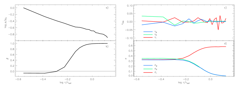
Figure 1.— We illustrate important initial condition information for an anisotropic system with a cuspy density profile ($\rho\propto r^{-1}$) and $Q_{0}=0.5$. The log-log density profile of the system is shown in panel a. Panel b shows the anisotropy profile. The average spherical component velocity profiles and velocity dispersion profiles are illustrated in panels c and d, respectively.

Figure 2.— Minimum axis ratios for the innermost 80% of mass in models that have initial radial anisotropy and virial ratios $Q_{0}\geq 0.2$. In each panel, models with $Q_{0}=1.0$ are denoted by square symbols, $Q_{0}=0.5$ models are marked with triangles, and systems with $Q_{0}=0.2$ are represented by diamonds. The empty symbols are derived from the NBODY2 simulations with $N=10^{4}$ particles, while the filled symbols represent Gadget-2 simulations with $N=10^{5}$ particles. The similar patterns followed by initially constant density models are shown in panels a) and b). Panels c) and d) show the similarities between axis ratio behavior in initially cuspy models. The same basic patterns also appear for initially Gaussian density models, panels e) and f). As the initial amount of radial velocity anisotropy increases, models become non-spherical.

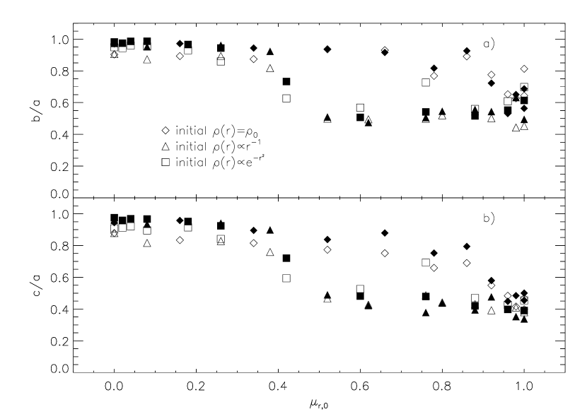
Figure 3.— Minimum 80%-mass axis ratios for cold $Q_{0}=0.1$, initially anisotropic systems. As in Figure 2, the open and closed symbols refer to evolved with NBODY2 and Gadget-2, respectively. The cuspy and Gaussian models (denoted by triangles and squares, respectively) follow the same basic trend for both $\frac{b}{a}$ and $\frac{c}{a}$. Models with initially constant density (represented by diamonds) do not show much variation with $\mu_{r}$, but these systems represent the remnants of models with significant mass loss.

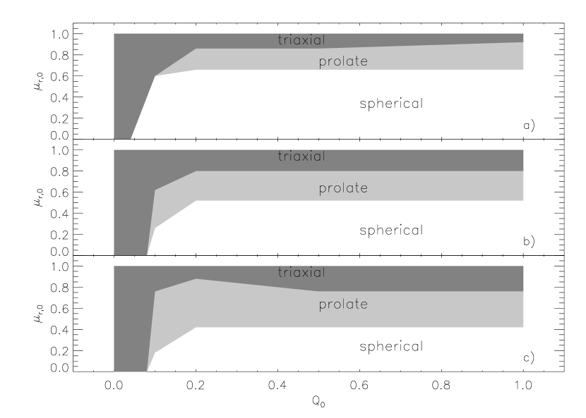
Figure 4.— A visual summary of the global behavior of the ROI for initially isotropic and anisotropic models. Panels a, b, and c correspond to models with constant, cuspy, and Gaussian initial density profiles, respectively. Models with initial conditions in the dark gray areas will evolve to triaxial shapes at the peak of the ROI. Initial conditions in the light gray region result in prolate systems. Systems that start from the unshaded region will remain more-or-less spherical throughout their evolutions. For the constant models in panel a, note that the models with $Q_{0}\lesssim 0.1$ had significant amounts of mass loss. The shape of the final virialized system refers only to the remnant, and drawing strong conclusions about the ROI from these cold models is problematic.

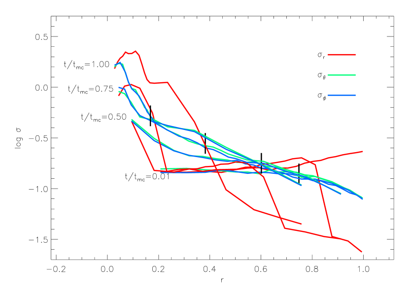
Figure 5.— Comparisons between spherical velocity component dispersions in a cuspy, initially radially anisotropic model with $r_{a}=0.9$ and $Q_{0}=0.1$. The overall behavior of the curves matches Figure 5b in Hozumi et al. (1996). The curves represent dispersions at four different times during the evolution up to the time of maximum collapse $t_{\rm mc}$. The earliest set of curves is essentially the beginning of the simulation, one-hundredth of the time to maximum collapse. The next set is halfway to collapse $t=0.5\>t_{\rm mc}$, the third set is for $t=0.75\>t_{\rm mc}$, and the upper-most curves show the situation at the time of maximum collapse. The vertical lines show the location of the half-mass radius at each interval. Note that the half-mass radius decreases as the time of maximum collapse is approached. With this level of initial anisotropy, the axis ratios do not reach their minimum values until many maximum collapse times have passed.

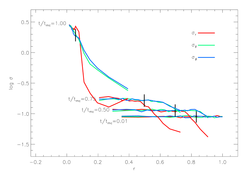
Figure 6.— Comparisons between spherical velocity component dispersions in the initially isotropic model with $Q_{0}=0.04$. The overall behavior of the curves matches Figure 3b in Hozumi et al. (1996). The curves shown have the same meaning as those in Figure 5. Again, take note that the half-mass radius marks move to the left in the figure as time increases. Axisratios typically reach their minimum values after roughly two—three maximum collapse time for these models.

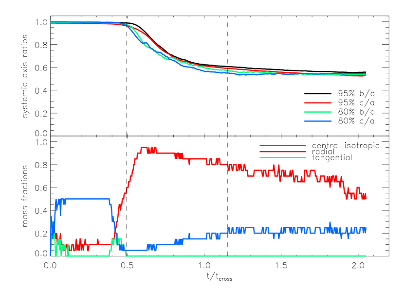
Figure 7.— The top panel shows the axis ratios as a function of time in the initially isotropic, Gaussian density profile system with $Q=0.00$. The behavior of the velocity mass fractions is plotted in the bottom panel. The vertical dashed lines mark the times at which a) left line, 55% of the system mass is on radially anisotropic orbits and b) right line, 20% of the central mass follows isotropic orbits.

Figure 8.— The logarithm of the growth factor $\hat{y}$ for an orbit in a high-time resolution simulation with $Q_{0}=0.00$ and an initially cuspy density profile. This particle is moving in a plane perpendicular to the intermediate axis of the bar at $t=1\>t_{\rm cross}$ (when the growth factor is 1). The orbit then experiences a roughly exponential growth perpendicular to the bar after which it settles into a quasi-periodic oscillatory phase. This behavior is reminiscent of orbits that undergo the instability discussed in Adams et al. (2007).

Figure 9.— The geometry of the toy model used to determine the torque on a test mass. The details of the model are described fully in Appendix A.

References

- Aarseth (2001) Aarseth, S. J. 2001, New Astronomy, 6, 277
- Adams et al. (2007) Adams, F. C., Bloch, A. M., Butler, S. C., Druce, J. M., Ketchum, J. A. 2007, ApJ, 670, 1027
- Barnes et al. (1986) Barnes, J., Goodman, J., Hut, P. 1986, ApJ, 300, 112
- Barnes et al. (2005) Barnes, E. I., Williams, L. L. R., Babul, A., Dalcanton, J. J. 2005, ApJ, 634, 775
- Barnes et al. (2007) Barnes, E. I., Williams, L. L. R., Babul, A., Dalcanton, J. J. 2007, ApJ, 654, 814
- Bellovary et al. (2008) Bellovary, J. M., Dalcanton, J. J., Babul, A., Quinn, T. R., Maas, R. W., Austin, C. G., Williams, L. L. R., Barnes, E. I. 2008, ApJ, 685, 739