Modeling the combined effect of surface roughness and shear rate on slip flow of simple fluids

Abstract

Molecular dynamics (MD) and continuum simulations are carried out to investigate the influence of shear rate and surface roughness on slip flow of a Newtonian fluid. For weak wall-fluid interaction energy, the nonlinear shear-rate dependence of the intrinsic slip length in the flow over an atomically flat surface is computed by MD simulations. We describe laminar flow away from a curved boundary by means of the effective slip length defined with respect to the mean height of the surface roughness. Both the magnitude of the effective slip length and the slope of its rate-dependence are significantly reduced in the presence of periodic surface roughness. We then numerically solve the Navier-Stokes equation for the flow over the rough surface using the rate-dependent intrinsic slip length as a local boundary condition. Continuum simulations reproduce the behavior of the effective slip length obtained from MD simulations at low shear rates. The slight discrepancy between MD and continuum results at high shear rates is explained by examination of the local velocity profiles and the pressure distribution along the wavy surface. We found that in the region where the curved boundary faces the mainstream flow, the local slip is suppressed due to the increase in pressure. The results of the comparative analysis can potentially lead to the development of an efficient algorithm for modeling rate-dependent slip flows over rough surfaces.

I Introduction

An adequate description of fluid flow over a solid boundary with surface roughness on multiple length scales often requires resolution of fine microscopic details of the flow structure while retaining peculiarities of a macroscopic picture Koumoutsakos05 . The most popular and practically important example is the problem of transport through heterogeneous porous media, which is an inherently multiscale system ConvPorMed . Modeling of the fluid flow at multiple scales is a nontrivial problem itself; however, it becomes much more difficult if one also needs to incorporate slip boundary conditions into equations of motion. Typically, a local slip appears if the wall-fluid interaction is sufficiently low, but the value of slip length (an extrapolated distance of the velocity profile to zero) generally depends not only on the surface energy and structure Churaev84 ; Charlaix01 ; Granick02 ; Leger06 ; Vinograd06 but on shear rate as well Granick01 ; Granick02 ; GranLang02 ; Breuer03 ; Ulmanella08 . Therefore, a correct form of the Navier-Stokes equation can be obtained only if the combined effect of surface roughness and shear rate on the slip length is taken properly into account. It is intuitively clear that the surface roughness and shear rate have an opposite impact on the slip length. A precise evaluation of relative contributions of these two factors is the subject of the present study.

The boundary conditions for the flow of monatomic fluids over atomically flat surfaces can be described in terms of the intrinsic slip length, which is defined as the ratio of the shear viscosity to the friction coefficient at the liquid/solid interface. The friction is determined by the strength of the interaction potential and molecular-scale corrugations of the crystalline wall. Recent MD studies Fischer89 ; KB89 ; Thompson90 ; Nature97 ; Barrat99 ; Barrat99fd ; Attard04 ; Priezjev05 ; Priezjev07 ; PriezjevJCP have reported values of the intrinsic slip length up to about a hundred molecular diameters for weak wall-fluid interaction energies. It is well established that the formation of commensurate structures of liquid and solid phases at the interface leads to stick boundary conditions Thompson90 ; Attard04 . The slip length decreases with increasing bulk pressure in the flow of nonwetting simple fluids over a smooth substrate Barrat99 . The MD simulations have also demonstrated that, depending on the wall-fluid interaction energy and the ratio of wall and fluid densities, the slip length is either relatively small (below a couple of molecular diameters) and shear-rate-independent Thompson90 or larger than several molecular diameters and increases with shear rate Nature97 ; Priezjev07 . Although several functional forms for the rate-dependent intrinsic slip length have been suggested for monatomic fluids Nature97 ; Fang05 ; Priezjev07 ; PriezjevJCP , as well as for polymer melts Priezjev04 ; Priezjev08 ; Niavarani08 ; LichPRL08 ; Priezjev09 , the rate-dependent boundary conditions were not used for modeling slip flows in complex geometries.

In contrast to the description of the flow over smooth boundaries (with microscopic surface roughness) by the intrinsic slip length, it is more appropriate to characterize the flow away from macroscopically rough surfaces by the effective slip length, which is usually defined with respect to the location of the mean roughness height. Recently, we investigated the behavior of the effective slip length in laminar flow over periodically corrugated surfaces for simple fluids Priezjev06 and polymer melts Niavarani08 . Both MD and continuum simulations have shown that the effective slip length decreases with increasing amplitude of the surface roughness. In the continuum analysis, the local (rate-independent) slip length is modified by the presence of boundary curvature Einzel90 ; Einzel92 and, therefore, becomes position-dependent along the wavy wall. A direct comparison between MD and continuum simulations at low shear rates demonstrated that there is an excellent agreement between the effective slip lengths for large wavelengths (above approximately 30 molecular diameters) and small wavenumbers $ka\lesssim 0.3$ Priezjev06 ; Niavarani08 . In the present paper, the analysis of the flow over a periodically corrugated surface is extended to higher shear rates and to the situation where the local slip length at the curved boundary is a function of both the radius of curvature and shear rate.

In the last decade, a number of studies have focused on the development of the hybrid continuum-atomistic methods to simulate fluid flows near smooth solid boundaries Thompson95 ; Feder00 , rough walls NieJFM04 , superhydrophobic surfaces GuoWei09 , corner flows NiePF04 , and flows near a moving contact line Hadji99 ; RenE05 . In multiscale algorithms, the time and length scales accessible in molecular simulations are considerably extended by employing the continuum method in the bulk region and applying the MD technique only near the interfaces. The two methods are coupled via constrained dynamics in an overlap region by matching mass, momentum and energy fluxes or velocity fields. The full MD simulations are then performed to validate the hybrid scheme. The drawback of the hybrid methods, however, is the cumbersome procedure for coupling of the two methods in the overlap region. The approach pursued in the present paper is different from that in the hybrid schemes. We first compute by MD simulations the intrinsic slip length as a function of shear rate in the flow over an atomically smooth surface. The Navier-Stokes equation is then solved numerically (in the whole computational domain) for the flow over a rough surface with the rate-dependent intrinsic slip length used as a local boundary condition. We found that the full MD simulations recover the continuum results at low and intermediate shear rates and small-scale surface roughness.

In this paper, the dynamic behavior of the effective slip length is investigated in steady shear flow over a periodically corrugated surface using molecular dynamics and continuum simulations. Both methods show that the effective slip length is nearly constant at low shear rates and it gradually increases at higher shear rates. The slight discrepancy between the effective slip lengths obtained from MD and continuum simulations at high shear rates is analyzed by examination of the local velocity and density profiles, as well as pressure and temperature distributions along the wavy surface. It is also shown by MD simulations that the singular behavior of the intrinsic slip length (in a flow over a smooth wall) at high shear rates is suppressed by the surface roughness.

The rest of this paper is organized as follows. The details of molecular dynamics and continuum simulations are described in the next section. The shear rate dependence of the intrinsic and effective slip lengths and the results of the comparative analysis are presented in Sec. III. The results are briefly summarized in the last section.

II The details of numerical methods

II.1 Molecular dynamics simulations

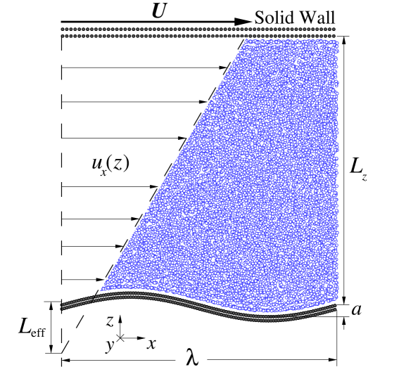
Figure 1: (Color online) The projection of $x$ and $z$ coordinates of the fluid monomers (open circles) confined between solid walls (filled circles). The atoms of the lower stationary wall are uniformly distributed along the sinusoidal curve with wavelength $\lambda$, amplitude $a$, and density $\rho_{w}\,{=}\,3.1\,\sigma^{-3}$. The shear flow is induced by the flat upper wall with the density $0.67\,\sigma^{-3}$ moving with a constant velocity $U$ in the $\hat{x}$ direction. The effective slip length $L_{\text{eff}}$ is computed by extrapolation of the velocity profile to $u_{x}=0$.

The system geometry and the definition of the effective slip length are illustrated in Fig. 1. The total number of fluid monomers in the cell is fixed to $N_{f}\!=16\,104$. The fluid monomers interact through the truncated pairwise Lennard-Jones (LJ) potential

$$V_{LJ}(r)=4\varepsilon\Big{[}\Big{(}\frac{\sigma}{r}\Big{)}^{12}-\Big{(}\frac{\sigma}{r}\Big{)}^{6}\Big{]},$$ (1)

where $\varepsilon$ is the energy scale and $\sigma$ is the length scale of the fluid phase. The cutoff radius for the LJ potential is set to $r_{c}=2.5\,\sigma$ for both fluid-fluid and wall-fluid interactions. The size of the wall atoms is the same as fluid monomers. Wall atoms are fixed at the lattice sites and do not interact with each other.

The motion of the fluid monomers was weakly coupled to a thermal reservoir via the Langevin thermostat Grest86 . To avoid bias in the shear flow direction, the random force and friction terms were added to the equations of motion in the $\hat{y}$ direction, perpendicular to the plane of shear Thompson90 . The equations of motion for fluid monomers in all three directions are as follows:

$$m\ddot{x}_{i} = -\sum_{i\neq j}\frac{\partial V_{ij}}{\partial x_{i}}\,,$$ (2)

$$m\ddot{y}_{i}+m\Gamma\dot{y}_{i} = -\sum_{i\neq j}\frac{\partial V_{ij}}{\partial y_{i}}+f_{i}\,,$$ (3)

$$m\ddot{z}_{i} = -\sum_{i\neq j}\frac{\partial V_{ij}}{\partial z_{i}}\,,$$ (4)

where $\Gamma\,{=}\,1.0\,\tau^{-1}$ is a friction coefficient that regulates the rate of heat flux between the fluid and the heat bath, and $f_{i}(t)$ is the random force with zero mean and variance $2m\Gamma k_{B}T\delta(t)$ determined from the fluctuation-dissipation relation. Unless otherwise specified, the temperature of the Langevin thermostat is set to $T\,{=}\,1.1\,\varepsilon/k_{B}$, where $k_{B}$ is the Boltzmann constant. The equations of motion were integrated using the Verlet algorithm Allen87 with a time step $\Delta t\,{=}\,0.002\,\tau$, where $\tau\!=\!\sqrt{m\sigma^{2}/\varepsilon}$ is the characteristic time of the LJ potential.

The intrinsic slip length was computed at the lower flat wall composed out of two layers of the fcc lattice with density $\rho_{w}\,{=}\,\,3.1\,\sigma^{-3}$ and nearest-neighbor distance $d\,{=}\,0.77\,\sigma$ between atoms in the $xy$ plane. The partial slip is permitted along the lower boundary due to relatively low wall-fluid interaction energy $\varepsilon_{wf}\,{=}\,0.5\,\varepsilon$. The no-slip boundary condition is enforced at the flat upper wall with a lower density $0.67\,\sigma^{-3}$ by allowing the formation of commensurate structures of liquid and solid phases at the interface. The nearest-neighbor distance between wall atoms is $1.28\,\sigma$ in the ($111$) plane of the fcc lattice. The wall-fluid interaction energy $\varepsilon$ ensures the no-slip condition at the upper wall holds even at high shear rates. The cell dimensions are set to $L_{x}\,{=}\,42.34\,\sigma$ and $L_{y}\,{=}\,10.0\,\sigma$ parallel to the confining walls. The MD simulations were performed at a constant fluid density ($\rho\,{=}\,0.81\,\sigma^{-3}$) ensemble, i.e., the relative distance between the walls was always fixed to $L_{z}\,{=}\,41.41\,\sigma$ in the $\hat{z}$ direction. Periodic boundary conditions were applied along the $\hat{x}$ and $\hat{y}$ directions.

The effect of surface roughness on slip flow was investigated in the cell with a lower sinusoidal wall with wavelength $\lambda\,{=}\,L_{x}$ and amplitude $a\,{=}\,1.82\,\sigma$ (see Fig. 1). Special care was taken to make the lower corrugated wall with a uniform density $\rho_{w}\,{=}\,\,3.1\,\sigma^{-3}$ (by including additional rows of atoms along the $\hat{y}$ direction) so that the lattice spacing along the sinusoidal curve remained $d\,{=}\,0.77\,\sigma$.

The fluid monomer velocities were initialized using the Maxwell-Boltzmann probability distribution at the temperature $T\,{=}\,1.1\,\varepsilon/k_{B}$. After an equilibration period of about $2\times 10^{4}\,\tau$, the velocity and density profiles across the channel were averaged for about $2\times 10^{5}\,\tau$ within bins of $L_{x}\times L_{y}\times\Delta z$, where $\Delta z\,{=}\,0.01\,\sigma$. The location and dimensions of the averaging regions for the computation of the local velocity and density profiles will be specified in Sec. III.3.

II.2 Continuum simulations

The two-dimensional, steady-state and incompressible Navier-Stokes (NS) equation is solved numerically using the finite element method. The equation of motion based on these assumptions is written as follows:

$$\rho\textbf{u}\cdot\nabla\textbf{u}=-\nabla p+\mu\nabla^{2}\textbf{u},$$ (5)

where $\textbf{u}=u\,\hat{i}+v\,\hat{\!j}$ is the velocity vector, $\rho$ is the density of the fluid, and $p$ and $\mu$ are the pressure field and fluid viscosity, respectively.

The penalty formulation was implemented for the incompressible solution to avoid decoupling of the velocity and pressure terms Pepper . In the penalty formulation, the continuity equation, $\nabla\cdot\textbf{u}=0$, is replaced with a perturbed equation

$$\nabla\cdot\textbf{u}=-\frac{p}{\Lambda},$$ (6)

where $\Lambda$ is the penalty parameter, which enforces the incompressibility condition. For most practical situations, where computation is performed with double-precision $64$ bit words, a penalty parameter ($\Lambda$) between $10^{7}$ and $10^{9}$ is sufficient to conserve the accuracy Pepper . After substitution of the pressure term in Eq. (6) into Eq. (5), the modified momentum equation can be rewritten as follows:

$$\rho\textbf{u}\cdot\nabla\textbf{u}=\Lambda\nabla(\nabla\cdot\textbf{u})+\mu\nabla^{2}\textbf{u}.$$ (7)

The Galerkin method with rectangular bilinear isoparametric elements is used to integrate the Navier-Stokes equation Pepper ; Niavarani09 .

The boundary conditions are applied at the inlet, outlet, and upper and lower walls. The periodic boundary conditions are implemented along the $\hat{x}$ direction for the inlet and outlet. The boundary condition at the upper wall is always no-slip. A partial slip boundary condition is applied at the lower wall. In addition to the global coordinate system ($\hat{x},\hat{z}$), a local coordinate system ($\vec{t},\vec{n}$) is defined along the lower curved boundary with unit vectors $\vec{t}$ and $\vec{n}$ representing the tangential and normal directions, respectively. The tangential component of the fluid velocity in the local coordinate system can be computed as

$$u_{t}=L_{0}[(\vec{n}\cdot\nabla)\,u_{t}+u_{t}/R],$$ (8)

where $R$ is the local radius of curvature and $L_{0}$ is the intrinsic slip length at the flat liquid/solid interface Einzel92 . The radius of curvature $R$ is positive and negative for concave and convex regions, respectively. The second-order forward-differencing scheme was used to compute accurately the normal derivative of the tangential velocity $(\vec{n}\cdot\nabla)\,u_{t}$ at the lower boundary.

At the beginning of the simulation procedure, the boundary conditions at the upper and lower walls are set to no-slip. Then, the equations of motion are solved implicitly and the tangential velocities at the lower boundary are updated according to Eq. (8). In the next step, the updated velocities at the lower boundary are used as a new boundary condition and the equations of motion are solved again. The iterative process is repeated until a desired accuracy is achieved. The convergence rate of the solution was controlled by applying an under-relaxation factor of 0.001 for the boundary nodes. For all results reported in the present paper, the continuum simulations were performed with $150\times 150$ grid resolution. However, the accuracy of the results was also checked by performing a set of simulations using a finer grid $180\times 180$. The maximum error in the effective slip length due to the grid resolution is $L_{\text{eff}}/L_{z}=0.003$. The same error bars were reported in the previous study of laminar flow over a periodically corrugated surface with either no-slip or (rate-independent) slip boundary conditions Niavarani09 .

The averaged error of the solution is defined as

$$\text{error}=\Big{[}\sum^{N_{p}}_{i=1}\frac{\mid\textbf{u}_{i}^{n}-\textbf{u}_{i}^{n+1}\mid}{\mid\textbf{u}_{i}^{n+1}\mid}\Big{]}/N_{p},$$ (9)

where $N_{p}$ is the number of nodes in the computational domain, $\textbf{u}_{i}^{n}$ is the magnitude of the velocity at node $i$ and time step $n$, and $\textbf{u}_{i}^{n+1}$ is the magnitude of the velocity in the next time step. The solution is converged when $\text{error}\leqslant 10^{-9}$ and the tangential velocities along the lower boundary satisfy $u_{t}=L_{local}\frac{\partial u_{t}}{\partial n}$, where the local slip length is $L_{local}=(L_{0}^{-1}-R^{-1})^{-1}$ Einzel92 .

III Results

III.1 MD simulations: the intrinsic and effective slip lengths

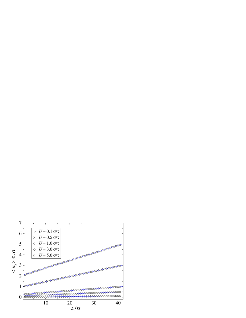
Figure 2: (Color online) Averaged velocity profiles for the tabulated upper wall speeds in the cell with flat upper and lower walls. The solid lines are the best linear fits to the data. The vertical axes indicate the location of the fcc lattice planes.

We first consider flow in the cell with flat upper and lower walls. The averaged velocity profiles are plotted in Fig. 2 for the selected upper wall speeds. The profiles are linear throughout the channel except for a slight curvature near the lower wall at $U\,{=}\,5.0\,\sigma/\tau$. Note that with increasing upper wall speed, the slip velocity at the lower wall increases monotonically up to about $2\,\sigma/\tau$ at $U\,{=}\,5.0\,\sigma/\tau$. The flow velocity at the top boundary remains equal to the upper wall speed due to the commensurability of liquid and solid structures at the interface and sufficiently high wall-fluid interaction energy. The shear rate was estimated from the linear slope of the velocity profiles across the entire cell.

The fluid viscosity computed from the Kirkwood relation Kirkwood is plotted in Fig. 3 as a function of shear rate in the cell with flat walls. In agreement with the results of previous MD studies on shear flow of simple fluids Nature97 ; Priezjev07 ; PriezjevJCP , the shear viscosity $\mu\,{=}\,2.15\pm 0.15\,\varepsilon\tau\sigma^{-3}$ remains rate-independent up to $\dot{\gamma}\tau\simeq 0.072$, which corresponds to the upper wall speed $U\,{=}\,5.375\,\sigma/\tau$. It is also known that at high shear rates the fluid temperature profiles become nonuniform across the cell and the heating up is larger near the interfaces Priezjev07 ; PriezjevJCP ; Priezjev08 . To ensure that the fluid viscosity is not affected by the heating up, we performed two additional sets of simulations at the upper wall speeds $U\,{=}\,1.0\,\sigma/\tau$ and $U\,{=}\,3.5\,\sigma/\tau$ and increased the temperature of the Langevin thermostat with an increment of $0.05\,\varepsilon/k_{B}$. In the range of the thermostat temperatures reported in Fig. 3, the shear viscosity is independent of temperature for both upper wall speeds. In Sec. III.3, the results of simulations performed at higher temperatures will be used to estimate the effect of pressure on the slip length.

The intrinsic slip length $L_{0}$ in the flow over a flat lower wall was determined from the linear extrapolation of velocity profiles to zero with respect to the reference plane located $0.5\,\sigma$ above the fcc lattice plane. The variation of the intrinsic slip length as a function of shear rate is presented in Fig. 4. At low shear rates $\dot{\gamma}\tau\lesssim 0.005$, the slip length is nearly constant. The leftmost data point reported in Fig. 4 is $\dot{\gamma}\tau\simeq 1.7\times 10^{-4}$ at the upper wall speed $U\,{=}\,0.01\,\sigma/\tau$. At higher shear rates, the intrinsic slip length first gradually increases and then grows rapidly as it approaches $\dot{\gamma}\tau\simeq 0.072$ when $U\,{=}\,5.375\,\sigma/\tau$. The behavior of the slip length in the flow over a flat wall can not be well described by the power law function suggested in Ref. Nature97 . Instead, a ninth-order polynomial function was used to fit the data (see the blue curve in Fig. 4). In the continuum analysis presented in the next section, the polynomial function will be used as a local (rate-dependent) boundary condition, Eq. (8), for the flow over a periodically corrugated wall.

When the upper wall speed becomes greater than $U\,{=}\,5.375\,\sigma/\tau$, the rate-dependence of the intrinsic slip length passes through a turning point at the maximum shear rate $\dot{\gamma}\tau\simeq 0.072$, and the slip length increases ($L_{0}\gg L_{z}$) while the shear rate decreases, leading to a negative slope of the rate-dependent curve (not shown). In this regime the slip velocity at the lower flat wall is greater than the fluid thermal velocity $v^{2}_{T}=k_{B}T/m$. The behavior of the intrinsic slip length at very large slip velocities was not considered further in the present study.

Next, the influence of surface roughness on the effective slip length is investigated in the flow over the lower corrugated wall with wavenumber $ka=2\pi a/\lambda=0.27$. The velocity profiles, averaged over the period of corrugation $\lambda\,{=}\,L_{x}$, are linear in the bulk of the film and curved near the lower wall within about $2\,a$ from the bottom of the valley (e.g., see Niavarani08 ; Niavarani09 ). Therefore, the effective slip length and shear rate were extracted from a linear fit to the velocity profiles inside the bulk region $10\leqslant z/\sigma\leqslant 30$. The effective slip length as a function of shear rate is also plotted in Fig. 4. Both the magnitude and slope of the rate-dependence of the effective slip length are reduced in comparison with the results for the flat wall. Following the rate-independent regime at $\dot{\gamma}\tau\lesssim 0.01$, the effective slip length increases monotonically up to a maximum value $L_{\text{eff}}(0.14\,\tau^{-1})\simeq 16.6\,\sigma$ at $U\,{=}\,8.0\,\sigma/\tau$.

At higher shear rates $\dot{\gamma}\tau\gtrsim 0.14$, the effective slip length starts to decrease with further increase in shear rate (see Fig. 4). We found, however, that the fluid temperature (density) becomes anomalously high (low) on the right side of the corrugation peak. For example, the fluid temperature in the region $0.5\lesssim x/\lambda\lesssim 0.9$ varies up to $Tk_{B}/\varepsilon\simeq\,1.6-1.85$ at $U\,{=}\,12.0\,\sigma/\tau$ (the rightmost point in Fig. 4). Also, the amplitude of the characteristic density oscillations normal to the curved boundary at $x/\lambda\simeq 0.43$ is reduced by about $40\%$ at $U\,{=}\,12.0\,\sigma/\tau$ in comparison with the fluid layering at equilibrium conditions (not shown). In the next section, the comparison between the effective slip lengths estimated from MD and continuum simulations is studied at shear rates $\dot{\gamma}\tau\lesssim 0.14$.

III.2 Comparison between MD and continuum simulations

In this section, we describe the behavior of the rate-dependent effective slip length computed from the solution of the Navier-Stokes equation. All variables in continuum simulations are normalized by the LJ length $\sigma$, time $\tau$, and energy $\varepsilon$ scales. The system is designed to mimic the MD setup. All nondimensional parameters in continuum simulations are marked by the ($\thicksim$) sign. The cell dimensions are set to $\tilde{L}_{x}\,{=}\,42.34$ and $\tilde{L}_{z}\,{=}\,40.41$ in the $\hat{x}$ and $\hat{z}$ directions, respectively. Similar to the MD setup, the wavenumber of the lower corrugated wall is fixed to $ka=0.27$. This value was chosen based on the previous analysis of the effective slip length in laminar flow of simple Priezjev06 and polymeric Niavarani08 fluids over a rough surface. It was shown Priezjev06 that at low shear rates there is an excellent agreement between the effective slip lengths extracted from MD and continuum simulations when a local (rate-independent) intrinsic slip length is used as a boundary condition along the wavy wall with $\lambda\gtrsim 30\,\sigma$ and $ka\lesssim 0.3$.

It is important to emphasize that in continuum simulations the intrinsic slip length in Eq. (8) is a function of the total shear rate at the curved boundary. The total shear rate is computed as a sum of the normal derivative of the tangential velocity $\partial u_{t}/\partial n$ and the ratio of the slip velocity to the radius of curvature $u_{t}/R$. The effective slip length is extracted from a linear part of the velocity profiles in the bulk region $10\leqslant\tilde{z}\leqslant 30$.

Figure 4 shows the effective slip length extracted from the continuum solution with the local rate-dependent intrinsic slip length at the lower corrugated boundary. The upper wall speed is varied in the range $0.025\leqslant\tilde{U}\leqslant 6$. As expected, the effective slip length obtained from the continuum simulations agrees well with the MD results at low shear rates $\dot{\gamma}\tau\lesssim 0.01$ where $L_{0}$ is nearly constant. With increasing shear rate up to $\dot{\gamma}\tau\lesssim 0.1$, the effective slip length increases monotonically. There is an excellent agreement between the two methods at intermediate shear rates $0.01\lesssim\dot{\gamma}\tau\lesssim 0.04$. At higher shear rates, $0.04\lesssim\dot{\gamma}\tau\lesssim 0.1$, the continuum predictions slightly overestimate the MD results. The maximum discrepancy in the effective slip length is about $2.5\,\sigma$ at $\dot{\gamma}\tau\simeq 0.1$, which corresponds to the upper wall speed $\tilde{U}=6.0$. For $\tilde{U}>6.0$, the local shear rate at the crest of the lower boundary, $[(\vec{n}\cdot\nabla)\,u_{t}+u_{t}/R]$, becomes larger than the highest shear rate, $\dot{\gamma}\tau\simeq 0.072$, achieved in the MD simulations for the intrinsic slip length (see Fig. 4), and, therefore, the local boundary condition, Eq. (8), cannot be applied.

III.3 A detailed analysis of the flow near the curved boundary

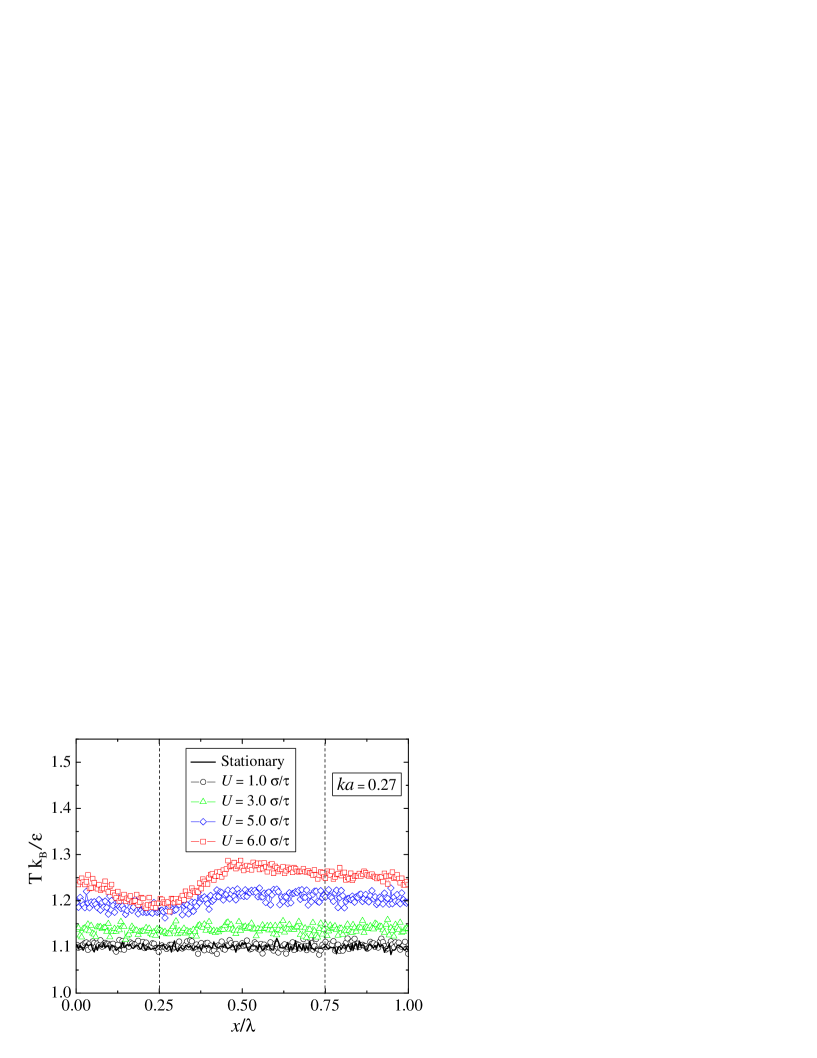
Figure 5: (Color online) Temperature of the first fluid layer $T(x)$ (in units of $\varepsilon/k_{B}$) along the lower corrugated wall ($ka=0.27$) for the indicated upper wall speeds. The vertical dashed lines denote the location of the crest ($x/\lambda=0.25$) and the bottom of the valley ($x/\lambda=0.75$).

In order to determine what factors cause the discrepancy between the effective slip lengths obtained from MD and continuum simulations at high shear rates, we performed a detailed analysis of the fluid temperature, pressure, density and velocity profiles near the lower boundary. The fluid temperature in the first fluid layer along the lower wall is plotted in Fig. 5 for the indicated upper wall speeds. As expected, at low shear rates $\dot{\gamma}\tau\lesssim 0.019$ ($U\lesssim 1.0\,\sigma/\tau$), the fluid temperature remains equal to the value $T\,{=}\,1.1\,\varepsilon/k_{B}$ set in the Langevin thermostat. With increasing upper wall speed, the temperature increases and eventually becomes nonuniformly distributed along the curved boundary (see Fig. 5). Somewhat surprisingly, we find that at high upper wall speeds $U\geqslant 5.0\,\sigma/\tau$ the fluid temperature is lowest above the crest even though the slip velocity in this region is expected to be higher than in the other locations.

The normal pressure distribution along the lower corrugated wall is shown in Fig. 6 for the selected upper wall speeds. Each data point represents the ratio of the averaged normal force on the wall atoms from the fluid monomers (within the cutoff radius) to the surface area $0.77\,\sigma\times 10.0\,\sigma$ in the $ty$ plane. The small variation of the pressure at equilibrium is due to the boundary curvature, i.e., the number of fluid monomers within the cutoff distance from the wall atoms is on average slightly larger above the peak than inside the valley. With increasing upper wall speed, the normal pressure increases in the valley ($x/\lambda\lesssim 0.12$ and $x/\lambda\gtrsim 0.54$) while it becomes smaller than the equilibrium pressure on the right slope of the peak (see Fig. 6). The normal pressure distribution extracted from the solution of the NS equation (not shown) is qualitatively similar to the profiles presented in Fig. 6. However, in the region $x/\lambda\gtrsim 0.54$ the MD data overestimate the continuum predictions for the pressure distribution at $U\gtrsim 3.0\,\sigma/\tau$ due to the increase in fluid temperature (see Fig. 5). It is clear from Fig. 6 that at higher upper wall speeds there is a considerable deviation from the equilibrium pressure, which can affect the local intrinsic slip length along the curved boundary (see discussion below). We finally comment that the normal pressure on the flat lower wall ($ka=0$) at equilibrium is equal to $P\simeq 2.36\,\varepsilon/\sigma^{3}$ (which agrees well with the pressure on the locally flat surface at $x/\lambda\simeq 0.5$ for $U=0$ in Fig. 6) and it increases up to $P\simeq 2.52\,\varepsilon/\sigma^{3}$ at the highest upper wall speed $U\,{=}\,5.375\,\sigma/\tau$.

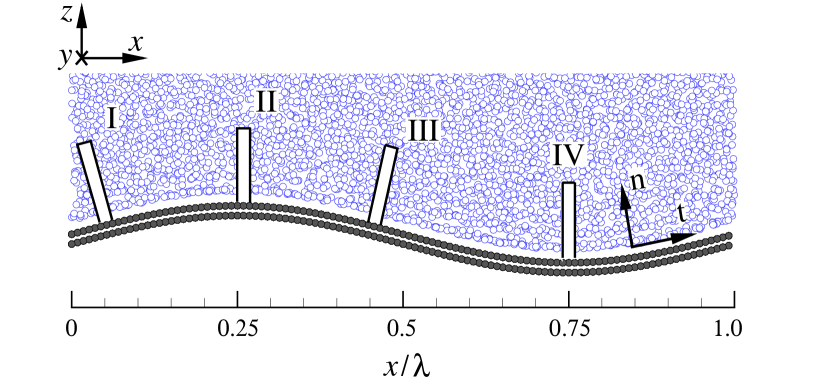
Figure 7: (Color online) A snapshot of the fluid monomers (open circles) near the lower corrugated wall (filled circles) with wavenumber $ka=0.27$. The rectangular boxes denote averaging regions on the left side of the peak (I) ($x/\lambda\simeq 0.05$), above the crest (II) ($x/\lambda\simeq 0.25$), on the right side of the peak (III) ($x/\lambda\simeq 0.45$), and at the bottom of the valley (IV) ($x/\lambda\simeq 0.75$). The unit vectors $\vec{t}$ and $\vec{n}$ indicate the tangential and normal directions at the boundary.

A snapshot of the flow near the lower corrugated wall is shown in Fig. 7, where the rectangular boxes illustrate the location of the averaging regions along the surface. The dimensions of the boxes are $d\,{=}\,0.77\,\sigma$, $5.0\,\sigma$, and $L_{y}\,{=}\,10.0\,\sigma$ along the curved boundary ($xz$ plane), normal to the curved boundary ($xz$ plane), and in the $\hat{y}$ direction, respectively. The velocity and density profiles discussed below were averaged inside the boxes within bins of thickness $0.01\,\sigma$ in the direction normal to the surface.

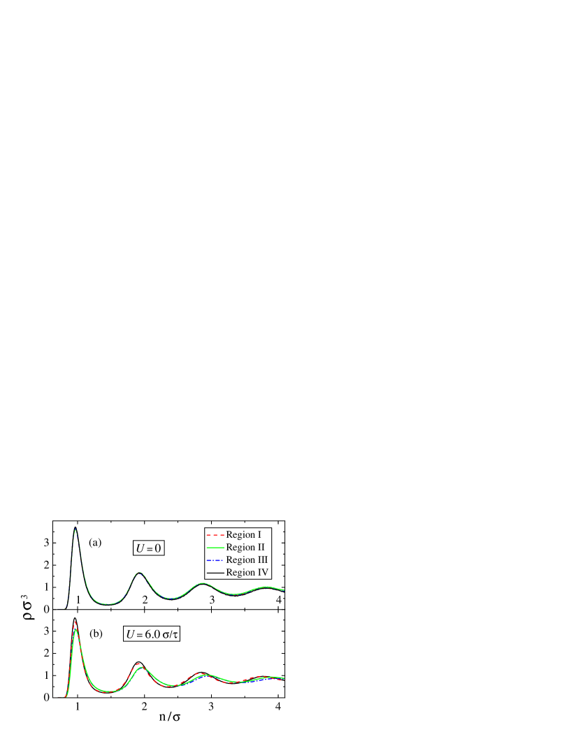
Figure 8: (Color online) Fluid density profiles averaged inside regions I–IV (shown in Fig. 7) near the corrugated lower wall with wavenumber $ka=0.27$. The upper wall speeds are $U=0$ (a) and $U\,{=}\,6.0\,\sigma/\tau$ (b).

In Figure 8 the averaged density profiles are plotted in regions I–IV for $U\,{=}\,0$ and $6.0\,\sigma/\tau$. In both cases, a pronounced fluid layering is developed near the lower wall. In the stationary case, Fig. 8 (a), the density profiles are almost the same in all four regions. Similar to the results of previous MD studies on slip flow over smooth surfaces Priezjev07 ; PriezjevJCP , when the upper wall speed increases, the contact density (magnitude of the first peak) is reduced due to a finite slip velocity along the curved boundary [see Fig. 8 (b)]. Among regions I–IV, it is expected that the local slip velocity is highest above the crest (region II) and lowest at the bottom of the valley (region IV), and, therefore, it is not surprising that the contact density in the region IV is larger than in the region II [see Fig. 8 (b)]. However, this correlation does not hold in regions I and III, where it is expected that at finite $Re$ the slip velocity in the region I would be larger than in the region III; but, as shown in Fig. 8 (b), the contact density in the region I is slightly larger than in the region III. Instead, we correlate this behavior with the nonuniform pressure distribution along the curved boundary where the local normal pressure in the region I is higher than in the region III (see Fig. 6). Note also that the location of the second and third fluid layers in regions II and III is slightly shifted away from the surface and the magnitude of the peaks is reduced due to the lower pressure in the region $0.2\lesssim x/\lambda\lesssim 0.5$ at $U\,{=}\,6.0\,\sigma/\tau$ in Fig. 6.

The local tangential velocity profiles normal to the curved boundary are presented in Fig. 9 for the upper wall speed $U\,{=}\,1.0\,\sigma/\tau$. Note that the profiles are almost linear away from the surface except for a slight curvature in the MD velocity profiles near the wall. The slip velocity above the crest (region II) is larger than in the other regions and $u_{t}$ at the bottom of the valley (region IV) is the lowest, as expected. The tangential velocity on the left side of the peak (region I) is larger than on the right side (region III) due to the inertial effects Niavarani09 . The tangential velocity $u_{t}$ and its normal derivative $\partial u_{t}/\partial n$ extracted from MD simulations in regions I, III, and IV agree rather well with the continuum results. Despite a slight overestimation of the continuum velocity with respect to the MD results above the crest (region II), the effective slip length is essentially the same in both methods for the upper wall speed $U\,{=}\,1.0\,\sigma/\tau$ (see the data at $\dot{\gamma}\tau\simeq 0.019$ in Fig. 4).

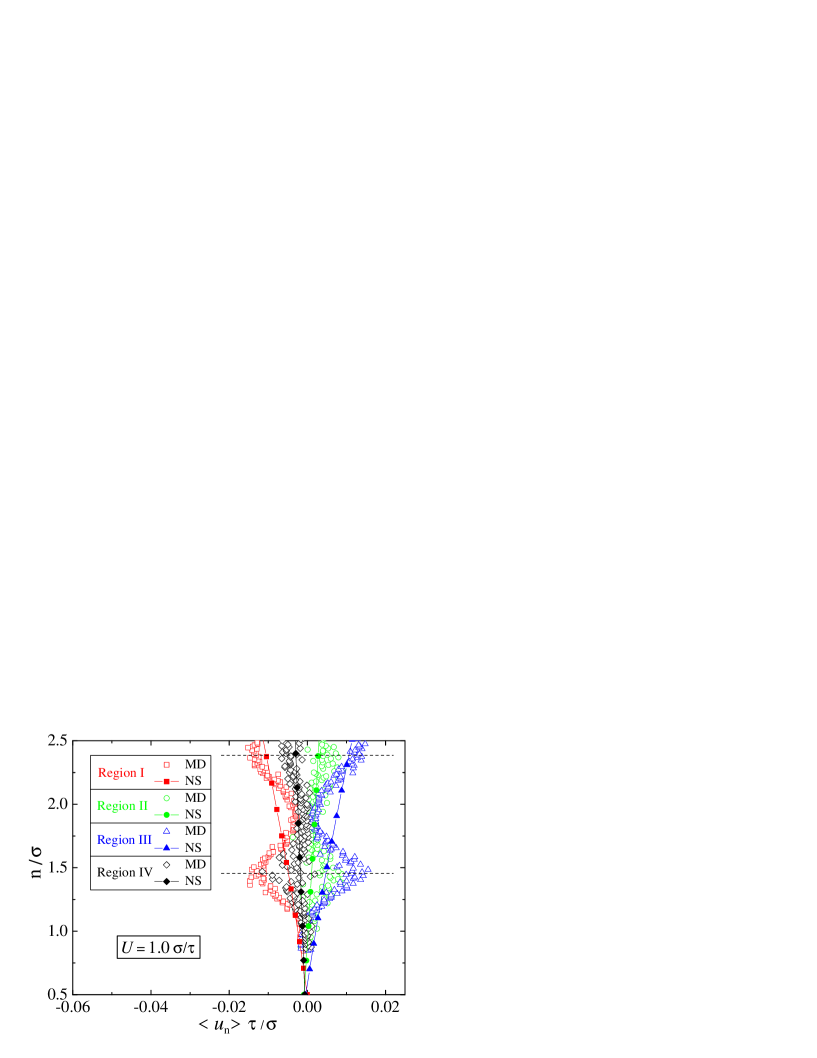
Figure 10: (Color online) Averaged normal velocity profiles inside regions I–IV (shown in Fig. 7) for the upper wall speed $U\,{=}\,1.0\,\sigma/\tau$. The profiles are extracted from MD simulations (open symbols) and the solution of the Navier-Stokes equation (filled symbols). The horizontal dashed lines indicate the location of the minima in density profiles (see text for details).

Figure 10 shows local profiles of the velocity component normal to the curved boundary for the upper wall speed $U\,{=}\,1.0\,\sigma/\tau$. Within statistical uncertainty, the normal velocities at the boundary are zero in both MD and continuum simulations. In regions I and IV the normal velocity is negative, while in regions II and III the velocity is positive away from the boundary. The negative and positive signs of the normal velocity are expected in regions I and III because of the positive and negative slopes of the boundary with respect to the shear flow direction. Although the boundary slope at the crest and at the bottom of the valley is parallel to the upper wall, the local symmetry of the flow with respect to $x/\lambda=0.25$ and $0.75$ is broken at finite Reynolds numbers ($Re\approx 15.6$ for $U\,{=}\,1.0\,\sigma/\tau$ in Fig. 10), and, as a result, the normal velocity in regions II and IV is not zero. Furthermore, the MD velocity profiles exhibit an unexpected oscillatory pattern away from the surface. These oscillations correlate well with the locations of the minima among the first three fluid layers [e.g., see Fig. 8(a)]. Visual inspection of the individual molecule trajectories indicates that the fluid monomers mostly undergo thermal motion within the moving layers but occasionally jump back and forward between the layers. The net flux between the layers, however, is not zero and its sign is determined by the direction of the flow near the boundary.

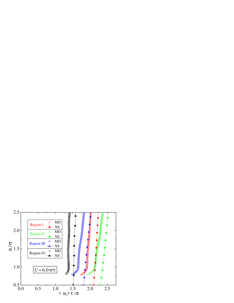
Figure 11: (Color online) Tangential velocity profiles averaged inside regions I–IV (shown in Fig. 7) near the lower corrugated wall. The upper wall speed is $U\,{=}\,6.0\,\sigma/\tau$. The velocity profiles are extracted from MD simulations (open symbols) and the solution of the Navier-Stokes equation (filled symbols).

The tangential velocity profiles averaged in regions I–IV at a higher upper wall speed $U\,{=}\,6.0\,\sigma/\tau$ are shown in Fig. 11. The flow pattern near the lower boundary is similar to that described in Fig. 9 for $U\,{=}\,1.0\,\sigma/\tau$, but the relative difference between the MD and continuum velocities is larger in each region which results in a maximum discrepancy between the effective slip lengths of about $2.5\,\sigma$ at $\dot{\gamma}\tau\simeq\,0.1$ in Fig. 4. We tried to estimate the local intrinsic slip length from the MD velocity profiles in regions I–IV and to compare $L_{0}$ with the continuum predictions. However, the normal derivative of the tangential velocity cannot be computed accurately because of the curvature in the velocity profiles and ambiguity in determining the range for the best linear fit. The resulting error bars associated with the linear extrapolation of the MD velocity profiles in Fig. 11 are greater than the maximum difference between MD and continuum results for $L_{\text{eff}}$ at high shear rates in Fig. 4. Instead, a more reliable data for the local intrinsic slip length (see Fig. 12) are obtained by computing the friction coefficient ($k_{f}=\mu/L_{0}$), which is the ratio of the wall shear stress to the slip velocity. The agreement between the MD and continuum results is quite good on the right side of the peak in Fig. 12. The intrinsic slip length computed from MD simulations is about $3-4\,\sigma$ smaller than the continuum $L_{0}$ on the left side of the peak due to higher fluid pressure in that region (see also discussion below).

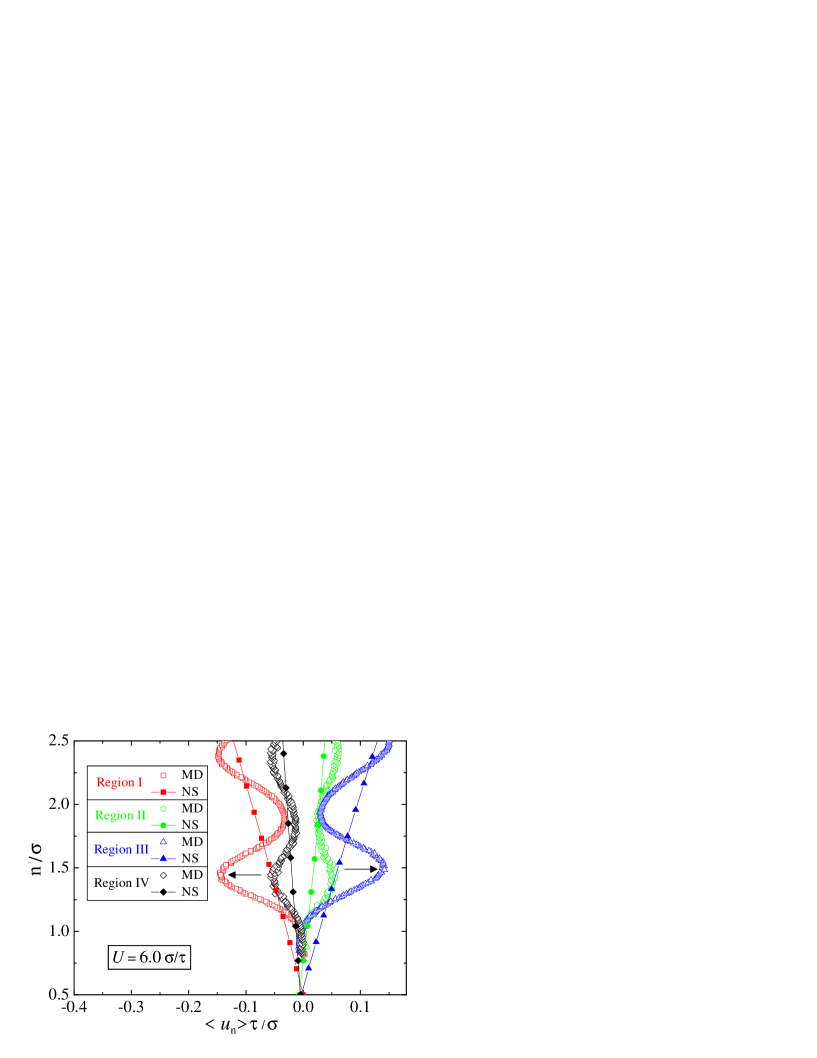
Figure 13: (Color online) Averaged normal velocity profiles inside regions I–IV obtained from MD simulations (open symbols) and the solution of the Navier-Stokes equation (filled symbols). The upper wall speed is $U\,{=}\,6.0\,\sigma/\tau$. The horizontal arrows indicate the location of the minima in density profiles between the first and second fluid layers in regions I and III.

The normal velocity profiles averaged in regions I–IV along the lower boundary are displayed in Fig. 13 for the upper wall speed $U\,{=}\,6.0\,\sigma/\tau$. In each region, the amplitude of oscillations in the MD velocity profiles is increased with respect to the mean flow predicted by the continuum analysis. Similar to the correlation between density and velocity profiles observed in Fig. 10 for $U\,{=}\,1.0\,\sigma/\tau$, the locations of the maxima in the normal velocity profiles in Fig. 13 correspond to the minima in the density profiles shown in Fig. 8 (b). At the higher upper wall speed, $U\,{=}\,6.0\,\sigma/\tau$, however, the location of the first peak in the velocity profile above the crest (region II) and on the right side of the peak (region III) is slightly displaced away from the boundary due to a small shift in the position of the second and third fluid layers in regions II and III [see Fig. 8 (b)].

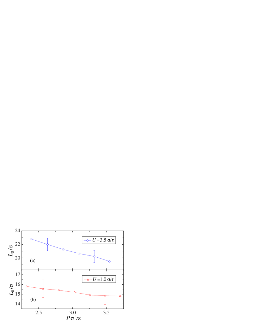
Figure 14: (Color online) The intrinsic slip length $L_{0}/\sigma$ as a function of the bulk pressure $P$ (in units of $\varepsilon/\sigma^{3}$) in the cell with flat upper and lower walls. The temperature of the Langevin thermostat is varied in the range $1.1\leqslant T\,k_{B}/\varepsilon\leqslant 1.35$ for the upper wall speed $U\,{=}\,3.5\,\sigma/\tau$ (a) and $1.1\leqslant T\,k_{B}/\varepsilon\leqslant 1.4$ for $U\,{=}\,1.0\,\sigma/\tau$ (b).

The effect of pressure variation along the curved boundary is not included in the rate-dependent intrinsic slip length, Eq. (8), used in continuum simulations. It was shown in Fig. 6 that at higher upper wall speeds, $U\gtrsim 3.0\,\sigma/\tau$, the fluid pressure along the lower corrugated wall deviates significantly from the equilibrium pressure. Next, we estimate the influence of pressure on the intrinsic slip length in shear flow over a flat wall by increasing the temperature of the Langevin thermostat. The MD simulations described in Sec. III.1 were repeated at the upper wall speeds $U\,{=}\,1.0\,\sigma/\tau$ and $3.5\,\sigma/\tau$ to examine $L_{0}$ at low ($\dot{\gamma}\tau\approx 0.018$) and high ($\dot{\gamma}\tau\approx 0.055$) shear rates. The results are presented in Fig. 14 for the indicated temperatures of the Langevin thermostat. As the bulk pressure increases, the intrinsic slip length is reduced by about $3\,\sigma$ at $U\,{=}\,3.5\,\sigma/\tau$ and about $\sigma$ at $U\,{=}\,1.0\,\sigma/\tau$. Note, however, that under these flow conditions the shear viscosity remains constant (see Fig. 3), and the variation of the friction coefficient ($k_{f}=\mu/L_{0}$) is determined only by the intrinsic slip length.

The maximum increase in pressure and the difference in $L_{0}$ reported in Fig. 14 (a) correlate well with the variation of pressure in Fig. 6 and the intrinsic slip length in Fig. 12 on the left side of the peak at $U\,{=}\,6.0\,\sigma/\tau$. We conclude, therefore, that the discrepancy between the effective slip lengths computed from MD and continuum simulations at high shear rates (shown in Fig. 4) is caused by the increase in fluid pressure on the left side of the peak (where the solid boundary faces the mainstream flow) and, as a result, the local intrinsic slip length is reduced. Thus, a more accurate continuum description of the slip flow over a curved boundary can be achieved by including the effect of pressure and temperature on the rate-dependent intrinsic slip length.

IV Conclusions

In this paper, molecular dynamics simulations were used to determine the intrinsic slip length as a function of shear rate in steady flow over an atomically flat surface. It was found, in agreement with previous MD studies, that the intrinsic slip length is nearly constant (rate-independent) at low shear rates and it grows rapidly as the shear rate approaches a critical value. In the presence of periodic surface roughness, the magnitude of the effective slip length is significantly reduced and its dependence on shear rate becomes less pronounced.

For the same surface roughness, the Navier-Stokes equation was solved numerically with the rate-dependent boundary conditions specified by the intrinsic slip length obtained from MD simulations. The continuum simulations reproduce accurately the MD results for the effective slip length at low and intermediate shear rates. The small difference between the effective slip lengths at high shear rates was analyzed by performing a detailed analysis of the local velocity fields and pressure distribution along the curved boundary. We found that the main cause of the discrepancy between MD and continuum results at high shear rates is the reduction of the local intrinsic slip length in the region of higher pressure where the boundary slope becomes relatively large with respect to the mainstream flow. These findings suggest that the continuum analysis of the flow over a rough surface at high shear rates should take into account the effect of pressure on the rate-dependent intrinsic slip length.

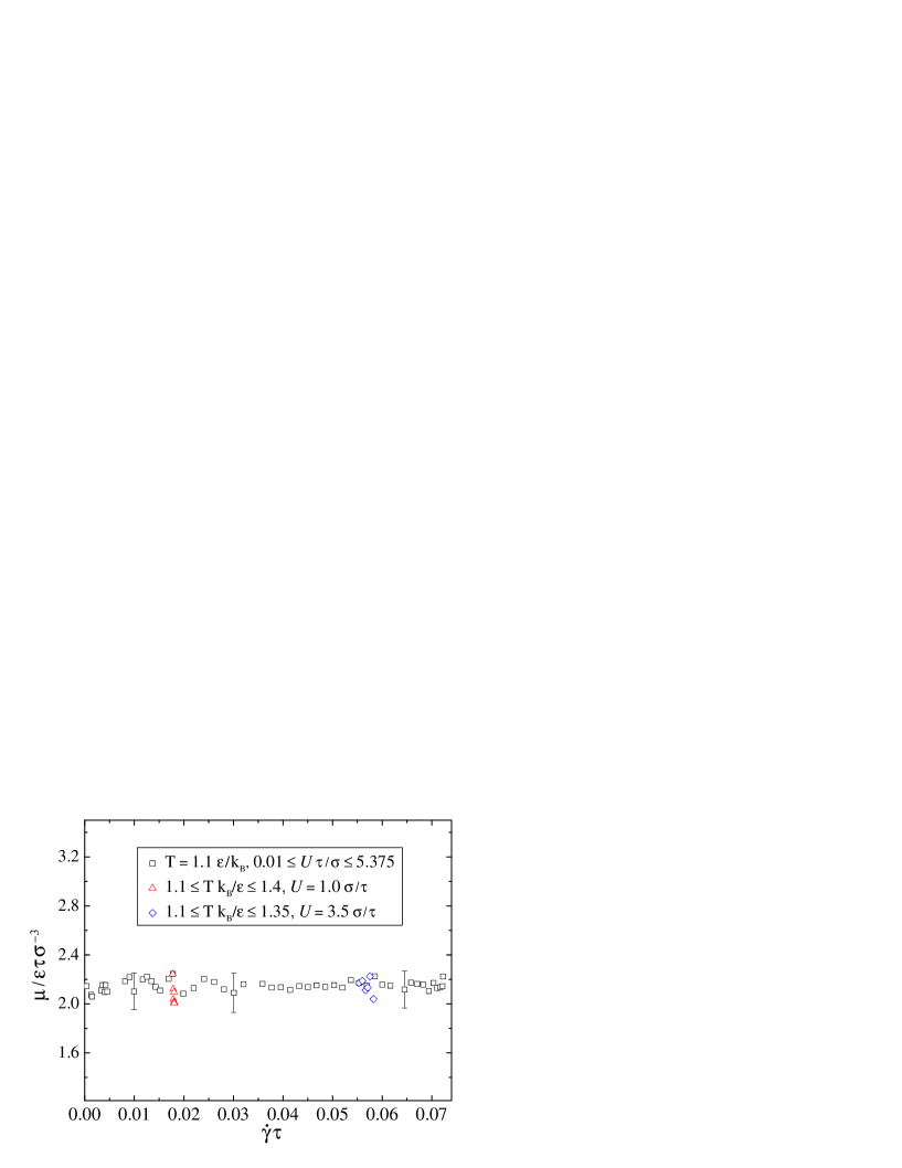
Figure 3: (Color online) Shear viscosity in the cell with flat upper and lower walls when the temperature of the Langevin thermostat is set to $T\,{=}\,1.1\,\varepsilon/k_{B}$ ($\Box$). Fluid viscosity as a function of the thermostat temperature $1.1\leqslant T\,k_{B}/\varepsilon\leqslant 1.4$ for the upper wall speed $U\,{=}\,1.0\,\sigma/\tau$ ($\triangle$) and $1.1\leqslant T\,k_{B}/\varepsilon\leqslant 1.35$ for $U\,{=}\,3.5\,\sigma/\tau$ ($\diamondsuit$).

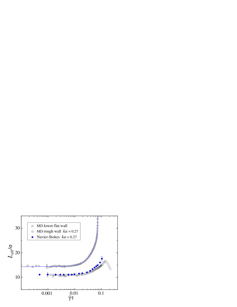
Figure 4: (Color online) The intrinsic slip length $L_{0}/\sigma$ as a function of shear rate for atomically flat walls ($\Box$). The blue solid curve is a ninth-order polynomial fit to the data. The effective slip length $L_{\text{eff}}/\sigma$ as a function of shear rate for the flow over the corrugated wall with wavenumber $ka=0.27$ ($\circ$). The effective slip length computed from the solution of the Navier-Stokes equation with the local rate-dependent slip length ($\bullet$).

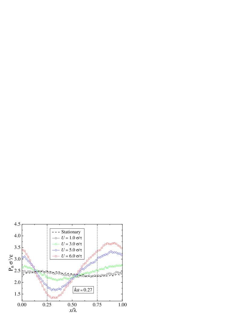
Figure 6: (Color online) The normal pressure $P_{n}$ (in units of $\varepsilon/\sigma^{3}$) along the lower corrugated wall ($ka=0.27$) for the selected upper wall speeds. The vertical dashed lines indicate the location of the crest ($x/\lambda=0.25$) and the bottom of the valley ($x/\lambda=0.75$).

Figure 9: (Color online) Averaged tangential velocity profiles inside regions I–IV obtained from MD simulations (open symbols) and the solution of the Navier-Stokes equation (filled symbols). The location of the averaging regions near the lower corrugated wall is shown in Fig. 7. The upper wall speed is $U\,{=}\,1.0\,\sigma/\tau$.

Figure 12: (Color online) The intrinsic slip length along the lower corrugated wall ($ka=0.27$) for the upper wall speed $U\,{=}\,6.0\,\sigma/\tau$. The data are obtained from MD simulations (open symbols) and the solution of the Navier-Stokes equation (filled symbols). The vertical dashed lines denote the position of the crest ($x/\lambda=0.25$) and the bottom of the valley ($x/\lambda=0.75$).

V Acknowledgments

- (1) P. Koumoutsakos, Annu. Rev. Fluid Mech. 37, 457 (2005).
- (2) D. A. Nield and A. Bejan, Convection in Porous Media (Springer, New York, 2006).
- (3) N. V. Churaev, V. D. Sobolev, and A. N. Somov, J. Colloid Interface Sci. 97, 574 (1984).
- (4) J. Baudry, E. Charlaix, A. Tonck, and D. Mazuyer, Langmuir 17, 5232 (2001).
- (5) Y. Zhu and S. Granick, Phys. Rev. Lett. 88, 106102 (2002).
- (6) T. Schmatko, H. Hervet, and L. Leger, Langmuir 22, 6843 (2006).
- (7) O. I. Vinogradova and G. E. Yakubov, Phys. Rev. E 73, 045302(R) (2006).
- (8) Y. Zhu and S. Granick, Phys. Rev. Lett. 87, 096105 (2001).
- (9) Y. Zhu and S. Granick, Langmuir 18, 10058 (2002).
- (10) C. H. Choi, K. J. A. Westin, and K. S. Breuer, Phys. Fluids 15, 2897 (2003).
- (11) U. Ulmanella and C.-M. Ho, Phys. Fluids 20, 101512 (2008).
- (12) U. Heinbuch and J. Fischer, Phys. Rev. A 40, 1144 (1989).
- (13) J. Koplik, J. R. Banavar, and J. F. Willemsen, Phys. Fluids A 1, 781 (1989).
- (14) P. A. Thompson and M. O. Robbins, Phys. Rev. A 41, 6830 (1990).
- (15) P. A. Thompson and S. M. Troian, Nature (London) 389, 360 (1997).
- (16) J.-L. Barrat and L. Bocquet, Phys. Rev. Lett. 82, 4671 (1999).
- (17) J.-L. Barrat and L. Bocquet, Faraday Discuss. 112, 119 (1999).
- (18) T. M. Galea and P. Attard, Langmuir 20, 3477 (2004).
- (19) N. V. Priezjev, A. A. Darhuber, and S. M. Troian, Phys. Rev. E 71, 041608 (2005).
- (20) N. V. Priezjev, Phys. Rev. E 75, 051605 (2007).
- (21) N. V. Priezjev, J. Chem. Phys. 127, 144708 (2007).
- (22) S. C. Yang and L. B. Fang, Molecular Simulation 31, 971 (2005).
- (23) N. V. Priezjev and S. M. Troian, Phys. Rev. Lett. 92, 018302 (2004).
- (24) A. Niavarani and N. V. Priezjev, Phys. Rev. E 77, 041606 (2008).
- (25) A. Niavarani and N. V. Priezjev, J. Chem. Phys. 129, 144902 (2008).
- (26) A. Martini, H. Y. Hsu, N. A. Patankar, and S. Lichter, Phys. Rev. Lett. 100, 206001 (2008).
- (27) N. V. Priezjev, Phys. Rev. E (2009). (cond-mat/0906.2771).
- (28) N. V. Priezjev and S. M. Troian, J. Fluid Mech. 554, 25 (2006).
- (29) D. Einzel, P. Panzer, and M. Liu, Phys. Rev. Lett. 64, 2269 (1990).
- (30) P. Panzer, M. Liu, and D. Einzel, Int. J. Mod. Phys. B 6, 3251 (1992).
- (31) S. T. O’Connell and P. A. Thompson, Phys. Rev. E 52, R5792 (1995).
- (32) E. G. Flekkøy, G. Wagner, and J. Feder, Europhys. Lett. 52, 271 (2000).
- (33) X. B. Nie, S. Y. Chen, W. E, and M. O. Robbins, J. Fluid Mech. 500, 55 (2004).
- (34) Q. Li and G.-W. He, Biomicrofluidics 3, 022409 (2009).
- (35) X. B. Nie, S. Y. Chen, and M. O. Robbins, Phys. Fluids 16, 3579 (2004).
- (36) N. G. Hadjiconstantinou, J. Comput. Phys. 154, 245 (1999).
- (37) W. Q. Ren and W. E, J. Comput. Phys. 204, 1 (2005).
- (38) G. S. Grest and K. Kremer, Phys. Rev. A 33, 3628 (1986).
- (39) M. P. Allen and D. J. Tildesley, Computer Simulation of Liquids (Clarendon, Oxford, 1987).
- (40) J. C. Heinrich and D. W. Pepper, Intermediate Finite Element Method: Fluid Flow and Heat Transfer Applications (Taylor and Francis, Philadelphia, 1999).
- (41) A. Niavarani and N. V. Priezjev, Phys. Fluids 21, 052105 (2009).
- (42) J. H. Irving and J. G. Kirkwood, J. Chem. Phys. 18, 817 (1950).
- (43) S. J. Plimpton, J. Comp. Phys. 117, 1 (1995); see also URL http://lammps.sandia.gov.