Integrating Post-Newtonian Equations on Graphics Processing Units

Abstract

We report on early results of a numerical and statistical study of binary black hole inspirals. The two black holes are evolved using post-Newtonian approximations starting with initially randomly distributed spin vectors. We characterize certain aspects of the distribution shortly before merger. In particular we note the uniform distribution of black hole spin vector dot products shortly before merger and a high correlation between the initial and final black hole spin vector dot products in the equal-mass, maximally spinning case. These simulations were performed on Graphics Processing Units, and we demonstrate a speed-up of a factor 50 over a more conventional CPU implementation.

I Introduction

With a number of gravitational wave detectors (LIGO Abbott:2007kva , Virgo Acernese:2008zza , TAMA Takahashi:2008zzb , and GEO600 Willke:2007zz ) now measuring signals at design sensitivity, the prospect of direct detection of gravitational radiation is becoming increasingly real and hence there is now a definite need to understand as much as possible about the most likely signal source – the stellar-mass binary black hole (BBH) system. Over recent years numerical relativity has reached the point were accurate and reliable inspiral and merger calculations can be produced by a number of different groups Aylott:2009tn . However, these calculations require significant computational effort, and the generation of a large-scale bank of numerical templates is currently intractable. Recent comparisons between numerical relativity and post-Newtonian (PN) approximate waveforms show good agreement surprisingly close to merger (up to a few orbits) boyle-2007 ; Hannam:2007wf , corresponding to a gravitational wave frequency of about $\omega_{\text{GW}}\approx 0.1$ or an orbital frequency of $\omega\approx 0.05$.

The main purpose of this work is to start a detailed study of the phase space of the PN equations of motion (see also Schnittman:2004vq ). We randomly choose initial conditions for those equations corresponding to circular orbits at some chosen orbital frequency $\omega_{0}$. We then integrate the PN equations of motion to some termination frequency $\omega_{f}$ shortly before merger, but in a region where the approximation has still been validated by numerical relativity. There are a number of interesting physical questions one can address in this context. It might be that there are certain configurations that are preferred shortly before merger. If so, maybe these regions should be studied using full numerical relativity. Another motivation regards partial information: If one had from some other observation (such as an electromagnetic counterpart) enough information about a BBH system long before merger to estimate a fraction of the parameters, it would be valuable to be able to estimate the system’s properties shortly before merger. For example, assume that the spin vector and mass of one BH have been measured, but only the mass of the other is known. Using an initially uniform distribution for the unknown spin vector an interesting question would be the final distribution of spin vectors shortly before merger. Would there be a uniform distribution or would it be strongly peaked, and how does it change given changes in the known parameters? We start to address some of these questions in this work, but much remains to be addressed in future research.

Another motivation for this work is provided by gravitational recoil. Numerical relativity has been able to obtain estimates for the gravitational recoil in unequal-mass Gonzalez:2006md ; Baker:2006vn ; Herrmann:2006ks and spinning 2007ApJ…661..430H ; 2007gr.qc…..1163K ; 2007ApJ…659L…5C configurations; in particular, extremely high recoil values have been obtained for specific configurations 2007ApJ…659L…5C ; Gonzalez:2007hi ; 2007gr.qc…..2133C . Initial studies using effective-one-body techniques have shown that very large kicks are unlikely to arise 2007astro.ph..2641S . Using the PN inspiral approach, it might be possible to predict the likelihood of certain configurations shortly before merger and then relate this result to the recoil using one of the many recoil formulas available in the literature.

To perform this study, we use the significant performance advantages of Graphics Processing Units (GPUs) to study the phase space of the BBH problem in a post-Newtonian (PN) setting. Each inspiral is described by a set of ordinary differential equations (ODEs) and the collection of inspirals are all decoupled. Therefore the computational problem is of the “embarrassingly parallel” kind, which is perfectly suited for GPUs. At this early stage in our studies, in which we focus on small portions of the full parameter space, the performance benefits provided by GPUs are not essential to perform the research. However, we anticipate that once we begin studies of larger sections of the parameter space the performance gains will become important.

II PN Equations of Motion

We integrate the post-Newtonian equations (Eqs. (1)-(4) and (9)) from Ref. Buonanno:2002fy (see Erratum Buonanno:2002erratum ), which describe a circular inspiral of 2 spinning BHs. The evolution is given by a system of coupled ODEs for the orbital frequency $\omega$, the individual spin vectors $\mathbf{S}_{i}$ for the 2 BHs, and the unit orbital angular momentum vector $\hat{\mathbf{L}}_{n}$.

$$\dot{\omega} = \omega^{2}\frac{96}{5}\eta(M\omega)^{5/3}\Bigg{\{}1-\frac{743+924\eta}{336}(M\omega)^{2/3}$$ (1)

$$-\left(\frac{1}{12}\sum_{i=1,2}\left(\chi_{i}\hat{\mathbf{L}}_{n}\cdot\hat{\mathbf{S}}_{i}(\frac{113m_{i}^{2}}{M^{2}}+75\eta)\right)-4\pi\right)M\omega$$

$$+\left(\frac{34103}{18144}+\frac{13661}{2016}\eta+\frac{59}{18}\eta^{2}\right)(M\omega)^{4/3}-\frac{1}{48}\eta\chi_{1}\chi_{2}\left(247(\hat{\mathbf{S}}_{1}\cdot\hat{\mathbf{S}}_{2})-721(\hat{\mathbf{L}}_{n}\cdot\hat{\mathbf{S}}_{1})(\hat{\mathbf{L}}_{n}\cdot\hat{\mathbf{S}}_{2})\right)(M\omega)^{4/3}$$

$$-\frac{1}{672}(4159+15876\eta)\pi(M\omega)^{5/3}+\Bigg{(}\left(\frac{16447322263}{139708800}-\frac{1712}{105}\gamma_{E}+\frac{16}{3}\pi^{2}\right)+(-\frac{273811877}{1088640}+\frac{451}{48}\pi^{2}-\frac{88}{3}\hat{\theta}\eta)\eta$$

$$+\frac{541}{896}\eta^{2}-\frac{5605}{2592}\eta^{3}-\frac{856}{105}log(16(M\omega)^{2/3})\Bigg{)}(M\omega)^{2}+(-\frac{4415}{4032}+\frac{358675}{6048}\eta+\frac{91495}{1512}\eta^{2})\pi(M\omega)^{7/3}\Bigg{\}}$$

$$\dot{\mathbf{S}_{i}} = \mathbf{\Omega}_{i}\times\mathbf{S}_{i}$$ (2)

$$\dot{\hat{\mathbf{L}}}_{n} = -\frac{(M\omega)^{1/3}}{\eta M^{2}}\frac{d\mathbf{S}}{dt}$$ (3)

where $d\mathbf{S}/dt=d\mathbf{S}_{1}/dt+d\mathbf{S}_{2}/dt$, $\gamma_{E}=0.577\ldots$ is Euler’s constant, and $\hat{\theta}=1039/4620$. The total mass is denoted by $M=m_{1}+m_{2}$ and $\eta=m_{1}m_{2}/M^{2}$ is the symmetric mass ratio. The magnitude of the angular momentum can be computed via $\left|\mathbf{L}_{n}\right|=\eta M^{5/3}\omega^{-1/3}$.

The evolution of the individual spin vectors $\mathbf{S}_{i}$ for the 2 BHs is described by a precession around $\mathbf{\Omega}_{i}$ with

$$\mathbf{\Omega}_{1}=\frac{(M\omega)^{2}}{2M}\left(\eta(M\omega)^{-1/3}(4+3\frac{m_{2}}{m_{1}})\hat{\mathbf{L}}_{n}+1/M^{2}(\mathbf{S}_{2}-3(\mathbf{S}_{2}\cdot\hat{\mathbf{L}}_{n})\,\hat{\mathbf{L}}_{n})\right)\,,$$ (4)

and $\mathbf{\Omega}_{2}$ is obtained by $1\leftrightarrow 2$. Note that the spin vectors $\mathbf{S}_{i}$ are related to the spin unit vectors $\hat{\mathbf{S}}_{i}$ via $\mathbf{S}_{i}=\chi_{i}m_{i}^{2}\hat{\mathbf{S}}_{i}$, i.e. $\chi_{i}\in[0,1]$ is the Kerr spin parameter of BH $i$. The system of coupled ODEs for $\omega,\hat{\mathbf{L}}_{n},$ and $\mathbf{S}_{i}$ given mass and spin parameters $m_{i},\chi_{i}$ are integrated from an initial frequency $\omega_{0}$ to a final frequency $\omega_{f}$. Typically, we choose $\omega_{0}$ corresponding to an initial separation of $r\approx 40M$ and $\omega_{f}=0.05$, which is a conservative estimate of where the PN equations still hold boyle-2007 ; Hannam:2007wf . Integrating the equations in a range of $\omega$ rather than $t$ provides a slightly more gauge-invariant measure to compare different systems.

The ODEs are integrated using the Dormand-Prince method. We set an error tolerance of $5\times 10^{-7}$ and start with an adaptive time step of size $h=10$.

The 2 initial spin vectors $\mathbf{S}_{i}$ span a 6-dimensional parameter space for each choice of parameters $m_{i},\omega_{0}$, and $\omega_{f}$. Note that the BBH problem is scale free, and we can therefore fix the total mass $M=m_{1}+m_{2}=1$ and need to study only the dependence on $m_{1}$. The last 2 parameters $\omega_{0}$ and $\omega_{f}$ are only interesting as consistency checks, and it is likely sufficient to analyze the situation for a few select choices. This still results in a challenging 7-dimensional ($m_{1}$ {1 dof}, $\mathbf{S}_{1}$ {3 dof}, and $\mathbf{S}_{1}$ {3 dof}, dof: degrees of freedom) problem. Here we break down the problem into a much more manageable 4-dimensional one by fixing not just $m_{i}$, but also the spin magnitudes $\chi_{i}$, which then means only the unit spin vectors $\hat{\mathbf{S}}_{i}$ are chosen freely. Each unit spin vector has only 2 degrees of freedom (since the third is given by the normalization condition).

III Notes on GPU computing

We use NVIDIA’s CUDA runtime and programming system cuda to implement the PN evolution code on GPUs. The GPUs today provide most impressive speed-ups over CPUs for single-precision computations. GPUs are primarily designed for computer games and hence current and future capabilities are essentially set by that market. This means it is unlikely that double-precision will be supported at similar speed-ups as single-precision. While double-precision arithmetic is now supported on some of the high-end cards, the performance gains over CPU codes are not very impressive and in our opinion do not yet justify the effort of porting the code to the CUDA infrastructure if double-precision is necessary throughout the code. Note that some results have been obtained where the code has been examined carefully and only a few critical computations where done in double-precision, providing most of the single-precision speed-up. By comparing single-precision and double-precision CPU results on a number of inspiral configurations we have verified single-precision is sufficient for our problem.

Porting the code to the CUDA architecture was relatively straightforward – we implemented the right-hand-side (RHS) computations of the ODEs on the GPU in a device kernel. The ODE integrator runs on the CPU and spawns kernels on the GPU, transferring the initial state. The full evolution is then performed on the GPU, including all necessary calculations of the RHS. At the end of the simulation, the state is transferred back to the CPU for output and analysis.

GPUs demonstrate significant global memory access latency (for the NVIDIA S1070, 400-600 cycles cuda ), and even worse access times are encountered for “non-coalesced” memory access. The latter is defined slightly differently on different NVIDIA GPU generations cuda , but for the latest generation it happens most frequently if multiple memory segments are accessed within a group of 16 threads called a half-warp. We have measured the non-coalesced memory stores and loads using the CUDA profiler and found no uncoalesced memory access, significantly simplifying the programming since this eliminates the need to avoid certain global memory access patterns using shared memory.

We found error detection and result verification on the GPU to be critical exercises. The computations on the GPUs are surprisingly resilient to errors happening on the cards. For instance, the on-board memory is not error correcting and kernel failures are not caught by default. This “error resilience” can lead to rather interesting failure modes from a scientific computing perspective. When too many inspirals are spawned simultaneously the runtime warns and terminates the program with an error message. As the number of inspirals is reduced a regime of “silent” failure is entered, where the program runs without any indication of error or warning, but it produces incorrect results. This can be caught by explicitly checking each kernel, but the runtime does not generate errors itself. Issues like this highlight the case for independent error checks for scientific computing.

We therefore decided to write our code in a multi-threaded way on the CPU. We first generate the random initial data for our inspiral studies on the GPU for the maximum number of parallel inspirals that can run successfully. We then transfer the initial data to the CPU and select a random subset of typically about 1% of these inspirals on the CPU. While the GPU is performing all the inspirals, we also evolve the selected inspirals on the CPU in double-precision in a separate CPU thread. After the GPU is done, we copy the data back to the CPU memory and compare the single-precision GPU data against the double-precision CPU data for the selected subset. This also validates that single-precision does not introduce unacceptable errors in this problem. We believe such cross checks are currently crucial for GPU computing. We want to stress however that we have not observed problems or errors once the initial ones were worked out.

IV Performance Results

We now evaluate performance advantages GPUs deliver in this context. We executed our code on a single core of the quad-core Intel Xeon E5410 CPU running at 2.33 GHz, which is rated at around 5 GFlops in double-precision. Note that the problem is “embarrassingly parallel,” so the CPU will be able to provide excellent scaling over the 4 cores. We integrated one of our test inspirals in the range $[\omega_{0}=0.004,\omega_{f}=0.1]$ 100 times serially and found we could achieve around 0.057 inspirals per millisecond (ms) on a single core.

For comparison, one of the four GPUs on our high-end unit (the NVIDIA Tesla S1070) is rated at 1035 GFlops in single-precision, delivering a theoretical performance advantage of about a factor 200 over the single-core CPU. We ran our test setup, spawning a large number of simultaneous inspirals in parallel.

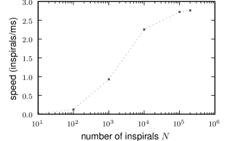
Figure 1: Performance of the GPU card. We vary the number of inspirals $N$ scheduled simultaneously on the GPU. For fewer than 100,000 inspirals peak performance is not reached, as there are not enough simultaneously executing threads to mask memory access latency. At 100,000 inspirals saturation is reached as the GPU works serially through the extra inspirals.

Fig. 1 shows results for the performance of the GPU card. As we increase the number of simultaneously scheduled inspirals $N$ the speed levels off at about 2.7 runs/ms. The GPU has 240 processors, which can work in parallel. Naively one would therefore expect the performance to improve until 240 inspirals are performed in parallel and after that the performance to level off as the processors need to work through the inspirals serially. However, the runtime CUDA scheduler has to be able to keep these 240 processors working simultaneously without waiting for memory access, which can be extremely slow. This is the likely reason why the performance still rises even after $N=10,000$, as the runtime has a better chance of squeezing the optimal performance out of the card by interleaving different inspirals without having to wait for costly memory transfers. We performed this study using block sizes of 256 threads. We found similar behavior with 128-thread blocks.

Based on this data, we achieve a very impressive speed-up of about a factor 50. While this comparison is slightly unfair to the CPU because we only use a single core and double-precision on the CPU, there is no doubt the performance gains are very significant. Note also that for this test problem we integrated the exact same problem in all cases. This means the individual threads run in perfect lock-step, the best possible case for the GPU. We typically see differences of about 10% in the runtime of different inspirals, and this would result in a slight inefficiency on the GPU as some of the threads in a block may finish before others. The double versus single-precision on the CPU has only a moderate effect, and the parallelization on the CPU will only be simple as long as the problem remains of the “embarrassingly parallel” type. We plan to extend our studies toward more dynamic explorations of phase space requiring dynamic feedback and communication between individual results. This would then require a significant implementation effort on the CPU in actually parallelizing the code, which is likely to be more difficult than the conversion to CUDA.

V Some Inspiral Results

In this section we highlight some of our findings from a completed initial study of the inspiral space. We emphasize that at this point we have focused on a few select situations only. We plan to soon move on to study larger regions of the initial configuration space and use more advanced statistical analysis tools to try to dynamically identify “interesting” regions.

For these simulations we integrate the ODEs Eq. (1)-(3) in the range $\omega_{0}=0.00395\rightarrow\omega_{f}=0.05$. The initial orbital frequency $\omega_{0}$ corresponds to a separation of $r\approx 40M$, and the final $\omega_{f}$ is chosen such that the gravitational wave frequency still matches numerical relativity results. We have varied both frequencies and, except in one case, have not found significant qualitative differences in the results. We leave detailed experimentation with different $\omega_{0}$ and $\omega_{f}$ as a topic of future study. The initial unit angular momentum is chosen as the unit vector in the z-direction $\hat{\mathbf{L}}_{n}=(0,0,1)$ without loss of generality.

For each choice of the black holes masses and spin magnitudes we sample in a uniform and random way their spin orientations. The latter corresponds to uniformly sampling a sphere, using the algorithm of Marsaglia:1972 . We use $N=100,000$ randomly selected initial spin orientations for each black hole. That is, a total of $N=10^{8}$ spin configurations.

In analyzing the data we have found the scalar products between the different unit vectors a useful quantity to investigate. This is also motivated by the crucial role these scalar products play in the recoil velocity.

V.1 Equal-mass, maximally spinning black holes

We start by looking at the case of two equal-mass ($m_{i}=0.5$), maximally spinning ($\chi_{i}=1$) black holes with randomly oriented initial unit-vector spin configurations. For this case all the pre-factors in the ODEs Eq. (1)-Eq. (3) for the spin terms are identical and the $\sum_{i}\chi_{i}\hat{\mathbf{L}}\cdot\hat{\mathbf{S}}_{i}$ term in the RHS for $\omega$ in particular simplifies to a form $\hat{\mathbf{L}}\cdot\mathbf{S}$ with $\mathbf{S}=\mathbf{S_{1}}+\mathbf{S_{2}}$. Note however that there is still a term of the form $\hat{\mathbf{S}}_{1}\cdot\hat{\mathbf{S}}_{2}$, which will change for the different configurations used.

As a first measure of the spin dynamics, we look at the scalar product between the two unit spin vectors $\hat{\mathbf{S}}_{1}\cdot\hat{\mathbf{S}}_{2}$ as well as the scalar products with the unit angular momentum $\hat{\mathbf{S}}_{i}\cdot\hat{\mathbf{L}}_{n}$. The simulations start out from an initially uniform distribution in each of these scalar products. Fig. 2 shows a histogram of the final value of $\hat{\mathbf{S}}_{1}\cdot\hat{\mathbf{S}}_{2}$ for $N=100,000$ inspirals and $N_{\text{bins}}=20$ bins. The figure also shows the probability density estimator for the final value of $\hat{\mathbf{S}}_{1}\cdot\hat{\mathbf{S}}_{2}$ at $\omega_{f}$, using a Gaussian kernel for different choices of the number of inspirals $N$. The density estimator is given by $\hat{p}(x)=1/(Nh)\sum_{j}^{N}K\left((x-x_{j})/h\right)$, where $h$ is the bandwidth and for the Gaussian kernel: $K\left((x-x_{i})/h\right)=1/\sqrt{2\pi}\exp\left(-(x-x_{i})^{2}/2h^{2}\right)$. We construct the bandwidth $h$ using $h=1.06\sigma N^{-1/5}$, where $\sigma$ is the standard deviation and $N$ is the number of inspirals Silverman86 . As $N$ is increased, the probability density estimator goes toward a uniform distribution. This shows that there is no structure in the final spin scalar product, i.e. that it is uniformly distributed. Note that the steep fall-off near the boundaries is an artifact of the estimator, which assumes the variable is distributed in the real line instead of $[-1,1]$ and smoothes out the discontinuous jump at $\pm 1$. This feature converges away in $N$. For $\hat{\mathbf{S}}_{i}\cdot\hat{\mathbf{L}}_{n}$ the distributions look very similar. In the equal-mass, maximum spin case there is no preferred angle between the spin vectors generated in the inspiral.

To further validate this even distribution of final dot product values, we used the Kolmogorov-Smirnov test to measure the uniformness of the final values. For this test, the BHs had equal mass and were non-maximally spinning, with $\chi_{i}=0.7$. We used a large sample containing 362,799,815 inspirals with random $\hat{\mathbf{S}}_{i}$ vectors over the unit sphere. The K-S test returned a p-value of $5.17\times 10^{-5}$, indicating a very uniform final distribution. The final histogram for this large test is displayed in Fig. 3, using $N_{\text{bins}}=100$ bins. It is visually apparent that no final dot product of the spin vectors is favored.

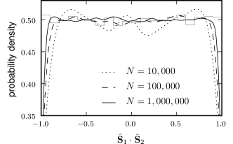
Figure 2: Uniform distribution of the scalar product $\hat{\mathbf{S}}_{1}\cdot\hat{\mathbf{S}}_{2}$ of the final configuration at $\omega_{f}$. The plot shows the convergence of the Gaussian kernel estimated probability density function for different $N$ towards the uniform distribution case (which would be at 0.5) as well as a histogram for the $N=100,000$ case.

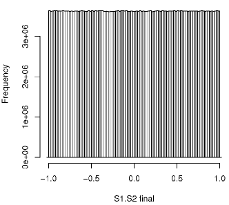
Figure 3: Uniform distribution of the scalar product $\hat{\mathbf{S}}_{1}\cdot\hat{\mathbf{S}}_{2}$ of the final configuration at $\omega_{f}$ when BH masses are even and $\chi_{i}=0.7$. The plot shows a histogram for the $N=362,799,815$ case.

While the final distribution in $\hat{\mathbf{S}}_{1}\cdot\hat{\mathbf{S}}_{2}$ remains uniform, we do find a high linear correlation between the initial and final values of this scalar product, as can be seen in Fig. 4. The latter shows a bivariate histogram for $(\hat{\mathbf{S}}_{1}\cdot\hat{\mathbf{S}}_{2})_{i}$ and $(\hat{\mathbf{S}}_{1}\cdot\hat{\mathbf{S}}_{2})_{f}$. Note that the histogram is normalized such that the maximum value is 1. We have also plotted the 0-contour line in light gray to make it easier to see how far configurations have spread. We have used $N_{\text{hist}}=79$ bins in each dimension, which was found by following the procedure in Ref. 2008arXiv0807.4820H and forcing equal numbers of bins in both dimensions.

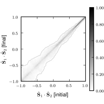
Figure 4: Final versus initial spin scalar product $\hat{\mathbf{S}}_{1}\cdot\hat{\mathbf{S}}_{2}$. The plot shows a high correlation in the scalar product between initial and final scalar product for the equal mass ($m_{1}=m_{2}=0.5$), maximally spinning ($\chi_{1}=\chi_{2}=1$) case. In light gray we show the 0-contour line to make it easier to see how far the configurations have spread.

This linear correlation can be quantified using the Pearson product-moment coefficient which is given by $r=1/(N-1)\sum_{i=1}^{N}\left((x_{i}-\bar{x})/\sigma_{x}\right)\left((y_{i}-\bar{y})/\sigma_{y}\right)$, where $\bar{x},\bar{y}$ are the sample means, $\sigma_{x},\sigma_{y}$ are the standard deviations, and $N$ is the number of inspirals. For the case of Fig. 4 we find $r=0.99$. Note that the correlations for $\hat{\mathbf{S}}_{1}\cdot\hat{\mathbf{L}}_{n}$ and $\hat{\mathbf{S}}_{2}\cdot\hat{\mathbf{L}}_{n}$ are not nearly as high, with $r=0.65$ for both cases. In Fig. 5 we show a similar histogram plot for $\hat{\mathbf{S}}_{1}\cdot\hat{\mathbf{L}}_{n}$. The case for $\hat{\mathbf{S}}_{2}\cdot\hat{\mathbf{L}}_{n}$ looks similar. The lower correlation is clearly visible compared to Fig. 4, as the values are much further spread from the diagonal in Fig. 5.

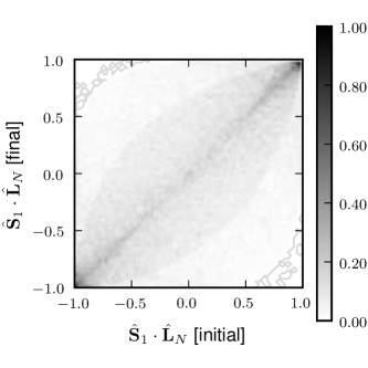
Figure 5: Final versus initial scalar product $\hat{\mathbf{S}}_{1}\cdot\hat{\mathbf{L}}_{n}$ for the same case as in Fig. 4. There is much less correlation between these initial and final scalar products compared to $\hat{\mathbf{S}}_{1}\cdot\hat{\mathbf{S}}_{2}$.

V.2 Unequal-mass, maximally spinning black holes

Having found the high correlation between the initial and final scalar products of spin vectors mentioned above we now change the mass $m_{1}$ of one BH while keeping $\chi_{1}=\chi_{2}=1$ and study the resulting change in correlation. In Fig. 6 we show the correlation coefficient $r$ of the initial and final values of $\hat{\mathbf{S}}_{1}\cdot\hat{\mathbf{S}}_{2}$ as the mass $m_{1}$ changes. Recall that we normalized the masses such that $M=m_{1}+m_{2}=1$, and hence $m_{1}\in[0,1]$.

Figure 6: The correlation coefficient $r$ of $(\hat{\mathbf{S}}_{1}\cdot\hat{\mathbf{S}}_{2})_{i}$ and $(\hat{\mathbf{S}}_{1}\cdot\hat{\mathbf{S}}_{2})_{f}$ for maximally spinning black holes as the mass of the bodies is changed. The correlation falls quickly as the masses become uneven.

Fig. 6 shows that the correlation drops quickly as the masses become uneven. This would indicate it would be harder to predict in a probabilistic sense the final value of this scalar product for a of a BBH inspiral in which the BHs have dissimilar masses and high spins.

V.3 Equal-mass, equal-spin, non-maximally spinning

Next we vary the spin $\chi$ for each black hole while keeping the same rate ($\chi_{1}=\chi_{2}$), and fixing the masses to be even ($m_{1}=m_{2}=0.5$) to see if there is a similar behavior in the correlation between $(\hat{\mathbf{S}}_{1}\cdot\hat{\mathbf{S}}_{2})_{i}$ and $(\hat{\mathbf{S}}_{1}\cdot\hat{\mathbf{S}}_{2})_{f}$ as we found when changing $m_{1}$. A similar behavior could be expected as the mass and spin parameters enter similarly in the spin evolution equations. However, as Fig. 7 shows, the correlation coefficient $r$ of the initial and final values of $\hat{\mathbf{S}}_{1}\cdot\hat{\mathbf{S}}_{2}$ remains constantly large ($r>0.98$), unlike the case of changing $m_{1}$ above. In Fig. 7 we also show the correlation coefficient $r$ for $\hat{\mathbf{S}}_{j}\cdot\hat{\mathbf{L}}_{n}$ ($j=1,2$), which shows significant variation.

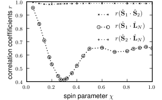
Figure 7: The correlation coefficient $r$ between the initial and final values of $\hat{\mathbf{S}}_{1}\cdot\hat{\mathbf{S}}_{2}$ and $\hat{\mathbf{S}}_{j}\cdot\hat{\mathbf{L}}_{n}$ ($j=1,2$). The masses are kept constant and equal ($m_{1}=m_{2}=0.5$) while the spin parameters are changed at the same rate, $\chi_{1}=\chi_{2}=\chi$. The correlation remains nearly constant and large for the $\hat{\mathbf{S}}_{1}\cdot\hat{\mathbf{S}}_{2}$ scalar product, but varies for $\hat{\mathbf{S}}_{j}\cdot\hat{\mathbf{L}}_{n}$.

In the case of $\hat{\mathbf{S}}_{j}\cdot\hat{\mathbf{L}}_{n}$ the behavior is similar for each $j$, which is expected since both BHs enter symmetrically into the expressions. The only difference between the BHs is their initial location.

V.4 $m_{1}=0.4$, equal-spin $\chi=0.05$

As an example of the rich structure that can be found if one leaves the equal mass case, we show in Fig. 8 a plot of the final versus initial spin scalar product $\hat{\mathbf{S}}_{1}\cdot\hat{\mathbf{S}}_{2}$ for the case of $m_{1}=0.4$, and $\chi_{1}=\chi_{2}=\chi=0.05$. In this case a ring-like structure appears in the scalar product and the data is now anti-correlated with $r=-0.14$. Though in other investigations presented in this paper the results were generally insensitive to the values of $\omega_{0}$ and $\omega_{f}$, we found in this case that the structure of the bivariate histogram could vary significantly based on these values. We leave a more full investigation of these cases to future work.

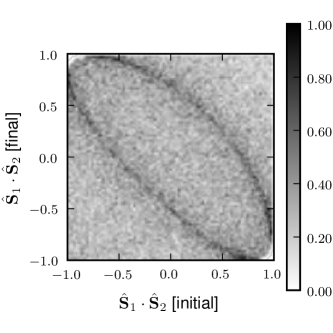
Figure 8: Final versus initial scalar product of spin vectors $\hat{\mathbf{S}}_{1}\cdot\hat{\mathbf{S}}_{2}$ for $m_{1}=0.4$ and equal-spin $\chi=0.05$ as an example of the richer structure away from highly symmetric cases. Note that the correlation is now negative.

VI Discussion

We have described our implementation of parallel integrations of the PN equations describing the circular inspiral of 2 black holes. Using the inherent parallelism of the problem of the inspiral space study of this system, we chose to implement this on Graphics Processors well adapted to the task. We achieved a speed-up of $50\times$ compared to a single-core CPU. This speed-up will be important for more advanced studies of large numbers of inspirals planned for the future.

First results from initial studies indicate there is a rich structure for certain regions of initial inspiral conditions. For an example see Fig. 8. In particular, the equal-mass case appears special, leading to more correlated dynamics compared to the equal-spin case. We used scalar products between the unit vectors to judge the dynamics.

For the future we plan to significantly expand our studies of the initial configuration space and to use more advanced statistical methods for analysis.

- [1] B Abbott et al. LIGO: The Laser Interferometer Gravitational-Wave Observatory. 2007.
- [2] F. Acernese et al. Status of Virgo. Class. Quant. Grav., 25:114045, 2008.
- [3] R. Takahashi et al. Operational status of TAMA300 with the Seismic Attenuation System (SAS). Class. Quant. Grav., 25:114036, 2008.
- [4] Benno Willke. GEO600: Status and plans. Class. Quant. Grav., 24:S389–S397, 2007.
- [5] Benjamin Aylott et al. Status of NINJA: the Numerical INJection Analysis project. Class. Quant. Grav., 26:114008, 2009.
- [6] Michael Boyle, Duncan A. Brown, Lawrence E. Kidder, Abdul H. Mroue, Harald P. Pfeiffer, Mark A. Scheel, Gregory B. Cook, and Saul A. Teukolsky. High-accuracy comparison of numerical relativity simulations with post-newtonian expansions. preprint (arXiv.org:0710.0158), 2007.
- [7] Mark Hannam, Sascha Husa, Bernd Brügmann, and Achamveedu Gopakumar. Comparison between numerical-relativity and post-Newtonian waveforms from spinning binaries: the orbital hang-up case. 2007.
- [8] Jeremy D. Schnittman. Spin-Orbit Resonance and the Evolution of Compact Binary Systems. Phys. Rev., D70:124020, 2004.
- [9] Jose A. Gonzalez, Ulrich Sperhake, Bernd Bruegmann, Mark Hannam, and Sascha Husa. Total recoil: the maximum kick from nonspinning black-hole binary inspiral. Phys. Rev. Lett., 98:091101, 2007.
- [10] J. G. Baker, J. Centrella, D.-I. Choi, M. Koppitz, J. R. van Meter, and M. C. Miller. Getting a Kick Out of Numerical Relativity. Ap. J. Lett., 653:L93–L96, December 2006.
- [11] F. Herrmann, I. Hinder, D. Shoemaker, and P. Laguna. Unequal-Mass Binary Black Hole Plunges and Gravitational Recoil. Class. Quant. Grav., 24:S33–S42, 2007.
- [12] F. Herrmann, I. Hinder, D. Shoemaker, P. Laguna, and R. A. Matzner. Gravitational Recoil from Spinning Binary Black Hole Mergers. Aptrophys J., 661:430–436, May 2007.
- [13] M. Koppitz, D. Pollney, C. Reisswig, L. Rezzolla, J. Thornburg, P. Diener, and E. Schnetter. Getting a kick from equal-mass binary black hole mergers. ArXiv General Relativity and Quantum Cosmology e-prints, January 2007.
- [14] M. Campanelli, C. Lousto, Y. Zlochower, and D. Merritt. Large Merger Recoils and Spin Flips from Generic Black Hole Binaries. Ap. J. Lett., 659:L5–L8, April 2007.
- [15] J. A. Gonzalez, M. D. Hannam, U. Sperhake, Bernd Bruegmann, and S. Husa. Supermassive kicks for spinning black holes. Phys. Rev. Lett., 98:231101, 2007.
- [16] M. Campanelli, C. O. Lousto, Y. Zlochower, and D. Merritt. Maximum gravitational recoil. ArXiv General Relativity and Quantum Cosmology e-prints, February 2007.
- [17] J. D. Schnittman and A. Buonanno. The Distribution of Recoil Velocities from Merging Black Holes. Ap. J. Lett., 662:L63–L66, June 2007.
- [18] Alessandra Buonanno, Yan-bei Chen, and Michele Vallisneri. Detecting gravitational waves from precessing binaries of spinning compact objects: Adiabatic limit. Phys. Rev., D67:104025, 2003.
- [19] Alessandra Buonanno, Yan-bei Chen, and Michele Vallisneri. Erratum: Detecting gravitational waves from precessing binaries of spinning compact objects: Adiabatic limit. Phys. Rev., D74:029905, 2006.
- [20] NVIDIA. http://www.nvidia.com, 2009.
- [21] George Marsaglia. Choosing a point from the surface of a sphere. The Annals of Mathematical Statistics, 43(2):645–646, 1972.
- [22] B.W. Silverman. Density Estimation. Chapman and Hall, 1986.
- [23] D. W. Hogg. Data analysis recipes: Choosing the binning for a histogram. ArXiv e-prints, July 2008.