Scaling Properties in Spatial Networks and its Effects on Topology and Traffic Dynamics

Abstract

Empirical studies on the spatial structures in several real transport networks reveal that the distance distribution in these networks obeys power law. To discuss the influence of the power-law exponent on the network’s structure and function, a spatial network model is proposed. Based on a regular network and subject to a limited cost $C$, long range connections are added with power law distance distribution $P(r)=ar^{-\delta}$. Some basic topological properties of the network with different $\delta$ are studied. It is found that the network has the smallest average shortest path when $\delta=2$. Then a traffic model on this network is investigated. It is found that the network with $\delta=1.5$ is best for the traffic process. All of these results give us some deep understandings about the relationship between spatial structure and network function.

Keyword: Spatial Network, Distance Distribution, Power Law, Traffic Process.

PACS: 89.75.Hc, 89.75.Da, 05.70.Jk

1 Introduction

In the last few years, the analysis and modeling of networked systems have received considerable attention within the physics community, including the World Wide Web, the Internet, and biological, social, and infrastructure networks[1, 2, 3]. Some of these networks exist only in an abstract network where the precise positions of the network nodes have no particular meaning, such as biochemical networks and social networks, while many others are different in which nodes have well-defined positions. In all kinds of network, a particular class is the spatial network embedded in the real space. Many networks belong to this class like the neural network[4], communication networks[5], electric power grid[6], transportation systems ranging from airport[7], street[8] , railway and subway[9] networks. Most of the previous works in the studies of complex network have focused on the characterization of the topological properties or other issues, while the spatial aspect has received more attention recently [10, 11, 12, 13].

Actually, the geography matters greatly. The geography information of the nodes and the distance between nodes would determine the characteristics of network and play an important role in the dynamics process happened on network more or less. Ignoring it would miss some of these systems’ interesting features. Empirical studies have revealed some interesting phenomena about the spatial structure of networks. One is the distance distribution of the links obeys power law. Examples include the Internet[14], social communication network[15] and online social network[16]. Recent research on circuit placement showed that the wire length of real circuits exhibits a power law distribution[17]. The anatomical distance distributions in human brain networks can also be well fitted by an exponentially truncated power-law[18]. More evidence comes from the empirical research on transportation networks. For Japanese airline networks[19], even there is an exponential decay in domestic flights, the distance distribution follows power-law when international flights are added. For the U.S. intercity passenger air transportation network[20], the distribution of link distance has a power-law tail with exponent is -2.2.

We also get the data of airline networks for Air China (CA) from its web site (http://www.airchina.com.cn). The network consists of 177 airports and 411 links including international flights. The distance distribution shows power law with exponent -2.38 (As shown in Fig.1 (a)). Another example is the express delivery network from a Chinese logistics company. It contains 301 cities and 421 undirected routes managed by the company. We examine the network in which the nodes are cities with more than one express services sector and the edges are the delivery route between cities. The networks’ lengths also show power-law distribution with exponents -1.87 (As shown in Fig.1 (b)).

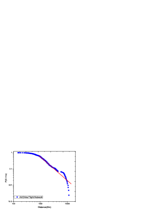
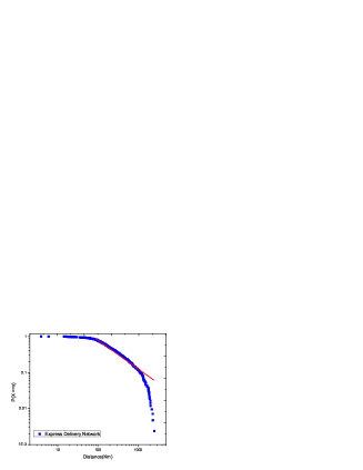
Figure 1: The edge length distribution of (a)the Air China airline network and (b)the express network

Why does the geographical embedded network possess this special spatial structure? How does the distance distribution affect the network’s function? All these problems are interesting. Analyzing these problems will help us understand the real spatial network deeply and benefit us for the design of transport system. The clue to answer these questions may rely on the consideration of costs and efficiency.

In spatial embedded networks, especially transport networks, the connection between nodes are restricted by cost constraints, reflected through the distance distribution. The cost of establishing long-range connections between distant spots is usually higher than the cost of establishing short-range connections. For electric power grids, the connection cost between farther spots is even higher, given that in long high-voltage lines a large amount of energy is lost during the transmission[21]. So we can easily understand that the number of short-range connections is much more than the long-range connections in these networks.

To demonstrate how the distance distribution of the connections affect the structure, function and the traffic dynamics process of the networks, we proposed a spatial network model in this paper. The model takes both the power law distribution of distance and the total cost of links into account. We construct spatially constrained networks embedded in geographical space, the distance distribution of the network obeys power law distribution $P(r)\propto r^{-\delta}$ and the network has a limited total cost $C$ to create links. We analysis the spatial network in detail, It shows that the network has the smallest average shortest path when $\delta=2$ and it isn’t influenced by the value of the total cost $C$ and the size of networks. Then the traffic model on the network is investigated. It is found that the network with $\delta=1.5$ is best for the traffic process. All of these results may explain why some of spatial networks’ exponent is close to 2, and the exponent of express delivery network is smaller than airline networks.

2 Spatial network model with limited total cost

Generally, the cost and efficiency are equally important in transport networks. The network structure is the result caused by the tradeoff between cost and efficiency.

The model network is embedded in a $k$-dimensional regular network. The long range connections is generated from a power law distance distribution by the approach suggested in[12]. Different from previous model[12], we introduce a total cost $C$ to this network model. Every link has a cost $c$ which is linear proportion to its distance $r$. For simplification and without lose any generalization, the edge cost $c_{i}$ is represented by its length $r_{i}$ in the model. The network is constructed under a certain limited total cost $C$. Then $L$ long range links with power law distance distribution are created under the condition $\sum^{L}_{i=1}r_{i}=C$. The network is constructed as following.

1. $N$ nodes are arranged in a $k$-dimensional lattice. Every node is connected with its nearest neighbors which can keep every node reachable. And, between any pair of nodes there is a well defined Euclidean distance.

2. A node $i$ is chosen randomly, and a certain distance $r(2\leq r\leq N_{max}$, $N_{max}$ is the largest distance between any nodes in the initial network.) from node $i$ is generated with probability $P(r)=ar^{-\delta}$, where $a$ is determined from the normalization condition $\sum^{N_{max}}_{r=2}P(r)=1$.

3. One of the $N_{r}$ nodes that are at distance $r$ from node $i$ is picked randomly, for example node $j$. An edge with distance weight $r$ between nodes $i$ and $j$ is created if there exist no edge between them. We make the multiple connections between two nodes excluded in this model.

4. Once the edge is created, a certain cost $c$ is generated. Repeat step 2 and 3 until the total cost reaches $C$.

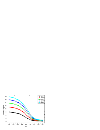
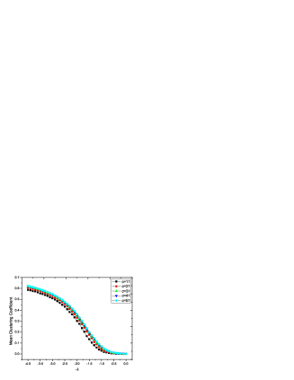
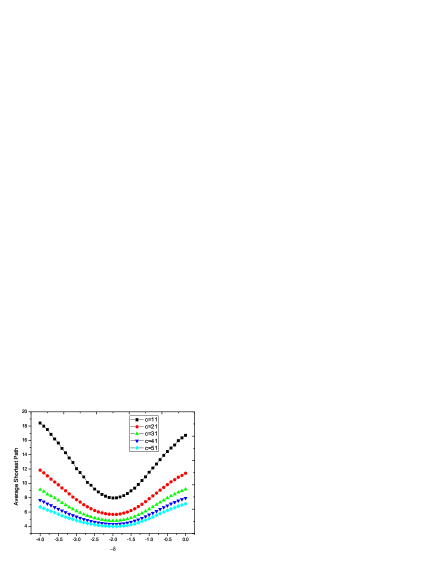
Figure 2: Basic topological properties in the model network. (a), (b), (c) represent the average degree, average clustering coefficient, and average shortest path on different total cost $C=500c(c=11,21,31,41,51)$ respectively. (c) shows that the average shortest path reaches minimum when $\delta=2$ with different total cost $C$.

In this model, the distance distribution and the total cost play important roles in the formation of the network. We first focus on how the topological properties are affect by the two factors. We are interested in how the power-law exponent $\delta$ influences the topological properties in the resulted binary network, including the average degree, mean clustering coefficient, and the average shortest path of the network. We have simulated the model both in 1-dimensional chain and 2-dimensional lattice, with periodic boundary condition respectively. They all give same qualitative results. So in the following, we only report the results of 1-dimensional chain with periodic boundary condition. The network size is typically $N=500$ and the results are the average of 1000 realizations. The total cost is set as $C=Nc(C=500c)$, where $c$ is the average cost per node and is set as 11, 21, 31, 41, 51 successively in the simulation. The results are shown in Figure.2. It shows that in the binary networks, the average degree and mean clustering coefficient decrease with the $\delta$. Interestingly, the average shortest path reaches its minimum when $\delta=2$. So when the total cost is limited, the network with $\delta=2$ has the lowest average shortest path, which may explain why the power-law exponent of distance distribution is close to 2 in many airline networks. As we know, in the public transport networks, travelers prefer less transfer when traveling. The transport network with $\delta=2$ has the lowest average shortest path in topological structure, which can make travelers have the least transfer and more convenience.

We also investigate how the total cost affects the networks properties. As we know, when the total cost reaches a certain value, the network with given size would become nearly full connected and the power law distance distribution will be destroyed. But in fact, the total cost $C$ is controlled by the average cost per node $c$ and it is generally limited, here we only focus on the effects of total cost in a reasonable range. When the power-law exponent be close to -4, in 2 or 3 dimensional space, the underlying network can not provide enough short long-range connections. It may result in drop-head phenomenon in the distance distribution. In this model, most of the long-range connections shows strict power law with drop-head in a small number of short long-range connections, which is prevalent in the real world. With the increasing of total cost, more long rang links are created. The average degree and mean clustering coefficient increase, while the average shortest path decreases. One interesting result is that for a certain range of total cost, the relationship between topological properties and the parameter $\delta$ keeps the same qualitatively as shown in Fig.2. Then, how this structure is related with the traffic dynamics? Next section will show us some results.

3 Traffic process on the model spatial network

From the analysis of the spatial network above, the average shortest path in the model network may explain why some public networks’s exponent close to 2 to a certain extent. What will happen when we consider the traffic dynamics on the above spatial embedded networks? To investigate the traffic dynamics may be helpful to understand that the express delivery network has a relatively smaller exponent in the distance distribution. The express delivery network is constructed based on all kinds of public transport networks, especially the airline networks. But it has its own feature, which is different from the public transport networks. First, the express delivery network is constructed from the perspective of overall optimization, while the public transport networks are constructed by self-organization, based on a local optimization process[22]. Second, the express delivery network cares really the traffic process on the network. Both efficiency and cost are important factors to shape the network structure. Third, same as the traffic model on networks, the bottleneck of the express network lies in the node, the capability of the node determine the whole network’s efficiency. So to investigate the traffic flow on such kind of network may help us to find how the exponent $\delta$ influences the traffic flow on the model network.

We employ a typical traffic dynamics[23] on this spatial network. Firstly, generate the underlying network infrastructure with the method we propose in last section. We also take the network as an binary one. Then a traffic dynamics is modeled on the network. All the nodes embedded on the spatial network are treated as both hosts and routers. We assume that every node can deliver at most $D$ packets one step toward their destinations. At each time step, there are $R$ packets generated homogeneously on the nodes in the system. The packets are delivered from their own origin nodes to destination nodes by special routing strategy. There are many kinds of different routing strategies, such as the shortest pathways routing strategy, the local dynamical strategy[24] and so on. Here the shortest pathways routing strategy is used. A packet, upon reaching its destination, is removed from the system. The order parameter

$$\eta(R)=\lim_{t\rightarrow\infty}\frac{1}{R}\frac{<\Delta N_{p}>}{\Delta t}$$ (1)

is used to characterize the phase transition. Here $\Delta N_{p}=N_{p}(t+\Delta t)-N_{p}(t)$, $<...>$ denotes taking the average over a time window of width $\Delta t$. $N_{p}(t)$ is the number of packets in the system at time $t$. We are most interested in the critical value $R_{c}$ (as measured by the number of packets created within the network per unit time), where a phase transition takes place from free flow to congested traffic. This critical value can best reflect the maximum capability of a system handling its traffic. In particular, for $R<R_{c}$, the numbers of created and delivered packets are balanced, leading to a steady free traffic flow. For $R>R_{c}$, traffic congestion occurs as the number of accumulated packets increases with time, simply because the capacities of the nodes for delivering packets are limited.

For simplicity, here we construct a network with 500 nodes under the total cost $C=500\times 11$ and $C=500\times 51$, and set every node has the same delivery ability $D=1$. We will adjust the network parameters $\delta$ to generate different networks, and then investigate how $\delta$ affects the critical value $R_{c}$ and the order parameter $\eta(R)$.

The simulation results for the critical value $\eta(R)$ as a function of $R$ on the model networks are reported in the Figure.3. It shows that the network with $\delta=1.5$ has a biggest $R_{c}$ and the smallest $\eta(R)$.

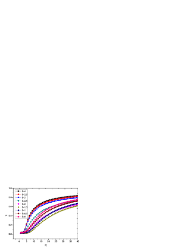
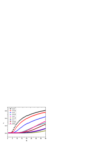
Figure 3: The simulation for the critical value $\eta(R)$ as $R$, different color mean for different $\delta$. The total cost C is 500$\times$11 in (a) and 500$\times$51 in (b). It shows that with different total cost, the network with $\delta=1.5$ is best for the traffic process.

In previous works, traffic handling capacity of a particular network has been estimated by a simple analysis method[23]. The betweenness coefficient of node $v$ can be calculated as $g(v)=\Sigma_{s\neq t}\frac{\sigma_{st}(v)}{\sigma_{st}}$. Here $\sigma_{st}$ is the number of shortest paths going from $s$ to $t$ and $\sigma_{st}(v)$ is the number of shortest paths going from $s$ to $t$ and passing through $v$. Note that with the increasing of parameter $R$ (number of packets generated every step), the system undergoes a continuous phase transition to a congested phase. Below the critical value $R_{c}$, there is no accumulation at any node in the network and the number of packets that arrive at node $u$ is $Rg_{u}/N(N-1)$ on average. Therefore, a particular node will collapse when $Rg_{u}/N(N-1)>D_{u}$ where $g_{u}$ is the betweenness coefficient and $D_{u}$ is the transferring capacity of node $u$. So, congestion occurs at the node with the largest betweenness. Thus $R_{c}$ can be estimated as $R_{c}=D_{u}N(N-1)/g_{max}$, where $g_{max}$ is the largest betweenness coefficient of the network.

In Fig.4 (a), the analysis results of $R_{c}$ with network parameters $\delta$ are shown. It indicates that this kind of network has the biggest $R_{c}$ when $\delta$ is close to 1.5, which is in good agreement with the simulation results as shown in Fig.4 (b).

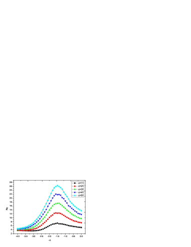
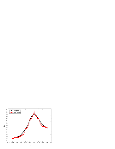
Figure 4: (a) shows the analytical results of $R_{c}$ with parameters $\delta$. The total cost $C$ increases from bottom-up. (b) shows the critical $R_{c}$ vs $\delta$ with the total cost $C=500\times 51$, both simulation and analysis indicate that the maximum $R_{c}$ corresponds to $\delta$=1.5.

4 Conclusions

In this paper, based on the empirical results about the power law distance distribution of some spatial networks, a spatial network model is studied. In a regular lattice, long range connections are added with the power law distance distribution $P(r)=ar^{-\delta}$ and a limited total cost. Some basic topological properties of the network generated by the model are investigated. It is found that the network has the smallest average topological shortest path when $\delta=2$. This may be the reason of the distance distribution in airport network shows power law with exponent close to 2, because people care more about the convenience and prefer less transfer when traveling by air. Then a traffic model is studied on the model network. We find that the network with $\delta=1.5$ is most conducive to the traffic process, although it has not the smallest average topological shortest path. This may explain why the power law exponent of the distance distribution in express transportation network is 1.87. Our results indicate that spatial constraints have an important influence on the transport networks and should be taken into account when modeling real complex systems.

References

- [1] R. Albert and A.-L. Barabási, Rev. Mod. Phys. 74, 47 (2002).
- [2] S. N. Dorogovtsev, J.F.F. Mendes, Adv. Phys. 51, 1079 (2002).
- [3] M. E. J. Newman, SIAM Rev. 45, 167 (2003).
- [4] O. Sporns, Complexity 8: 56-60 (2002).
- [5] V. Latora and M. Marchiori, Phys. Rev. E 71, 015103(R) (2005).
- [6] R. Albert, I. Albert and G.L. Nakarado, Phys. Rev. E 69, 025103 (2004).
- [7] R. Guimer , S. Mossa, A. Turtschi and L.A.N. Amaral, Proc. Natl. Acad. Sci. U.S.A. 102, 7794 (2005).
- [8] P. Crucitti, V. Latora and S. Porta, preprint physics/0504163.
- [9] V. Latora and M. Marchiori, Physica A 314, 109 (2002).
- [10] M. T. Gastner, and M.E.J. Newman, Eur. Phys. J. B 49, 247-252 (2006).
- [11] A. Cardillo, S. Scellato, V. Latora and S. Porta, Phys. Rev. E 73, 066107 (2006).
- [12] K. Kosmidis, S. Havlin and A. Bunde, Europhys. Lett. 82, 48005, (2008).
- [13] Y. Hayashi and J. Matsukubo, Phys. Rev. E 73, 066113 (2006).
- [14] S-H. Yook, H. Jeong and A-L. Barabási, Proc. Natl. Acad. Sci. U.S.A. 99, 13382 (2002).
- [15] R. Lambiotte, V. D. Blondel, C.d Kerchove, E. Huens, C. Prieur, Z. Smoreda and P.V Dooren, Physica A 387, 5317-5325 (2008).
- [16] D. Liben-Nowell, J. Novak, R. Kumar, P. Raghavan, and A. Tomkins, Proc. Natl. Acad. Sci. U.S.A. 102, 11623-11628 (2005).
- [17] J. Dambre, Prediction of interconnect properties for digital circuit design and technology exploration, Ph.D. dissertation: Ghent University, Faculty of Engineering (2003).
- [18] Y. He, Z. J. Chen and A. C. Evans, Cerebral Cortex 17(10):2407-2419, (2007).
- [19] Y. Hayashi, IPSJ Digital Courier, Vol.2, 155-164 (2006).
- [20] Z. Xu and R. Harriss, GeoJournal 73, 87-102 (2008).
- [21] R. Xulvi-Brunet and I. M. Sokolov, Phys. Rev. E 75, 046117 (2007).
- [22] M. Barthelemy, and A. Flammini, Phys. Rev. Lett. 100, 138702 (2008).
- [23] L. Zhao, Y.-C. Lai, K. Park, and N. Ye, Phys. Rev. E 71, 026125 (2005).
- [24] M.-B. Hu, R. Jiang, Y.-H. Wu, W.-X. Wang and Q.-S. Wu, Physica A 387, 4967-4972 (2008).