Distributed averaging via lifted Markov chains

Abstract

Motivated by applications of distributed linear estimation, distributed control and distributed optimization, we consider the question of designing linear iterative algorithms for computing the average of numbers in a network. Specifically, our interest is in designing such an algorithm with the fastest rate of convergence given the topological constraints of the network. As the main result of this paper, we design an algorithm with the fastest possible rate of convergence using a non-reversible Markov chain on the given network graph. We construct such a Markov chain by transforming the standard Markov chain, which is obtained using the Metropolis-Hastings method. We call this novel transformation pseudo-lifting. We apply our method to graphs with geometry, or graphs with doubling dimension. Specifically, the convergence time of our algorithm (equivalently, the mixing time of our Markov chain) is proportional to the diameter of the network graph and hence optimal. As a byproduct, our result provides the fastest mixing Markov chain given the network topological constraints, and should naturally find their applications in the context of distributed optimization, estimation and control.

shinAuthor names appear in the alphabetical order of their last names. All authors are with Laboratory for Information and Decision Systems, MIT. This work was supported in parts by NSF projects HSD 0729361, CNS 0546590, TF 0728554 and DARPA ITMANET project. Authors’ email addresses: {kmjung, devavrat, jinwoos}@mit.edu

1 Introduction

The recently emerging network paradigms such as sensor networks, peer-to-peer networks and surveillance networks of unmanned vehicles have led to the requirement of designing distributed, iterative and efficient algorithms for estimation, detection, optimization and control. Such algorithms provide scalability and robustness necessary for the operation of such highly distributed and dynamic networks. In this paper, motivated by applications of linear estimation in sensor networks [16, 6, 23, 31], information exchange in peer-to-peer networks [20, 26] and reaching consensus in unmanned vehicles [15], we consider the problem of computing the average of numbers in a given network in a distributed manner. Specifically, we consider the class of algorithms for computing the average using distributed linear iterations. In applications of interest, the rate of convergence of the algorithm strongly affects its performance. For example, the rate of convergence of the algorithm determines the agility of a distributed estimator to track the desired value [6] or the error in the distributed optimization algorithm [27]. For these reasons, designing algorithms with fast rate of convergence is of a great recent interest [6, 3, 10] and the question that we consider in this paper.

A network of $n$ nodes whose communication graph is denoted by $G=(V,E)$, where $V=\{1,\dots,n\}$ and $E=\{(i,j):i\mbox{~{}and~{}}j\mbox{~{}can communicate}\}$. Each node has a distinct value and our interest is designing a distributed iterative algorithm for computing the average of these numbers at the nodes. A popular approach, started by Tsitsiklis [31], involves finding a non-negative valued $n\times n$ matrix $P=[P_{ij}]$ such that

• $P$ is graph conformant, i.e. if $(i,j)\notin E$ then $P_{ij}=0$,

• $\mathbf{1}^{T}P=\mathbf{1}^{T}$, where $\mathbf{1}=[1]$ is the (column) vector of all components $1$,

• $P^{t}\mathbf{x}\to x_{\text{ave}}\mathbf{1}$ as $t\to\infty$ for any $\mathbf{x}\in\mathbb{R}_{+}^{n}$, where $x_{\text{ave}}=\left(\sum_{i=1}^{n}x_{i}\right)/n$.

This is equivalent to finding an irreducible, aperiodic random walk on graph $G$ with the uniform stationary distribution.

The quantity of interest, or the performance of algorithm, is the time it takes for the algorithm to get close to $x_{\text{ave}}\mathbf{1}$ starting from any $\mathbf{x}$. Specifically, given $P$, define the $\varepsilon$-computation time of the algorithm as

$$T_{\varepsilon}(P) = \inf\left\{t~{}:~{}\forall\mathbf{x}\in\mathbb{R}_{+}^{n},\frac{\|P^{t}\mathbf{x}-x_{ave}\mathbf{1}\|_{\infty}}{x_{ave}}\leq\varepsilon\right\}.$$ (1)

It is well-known that $T_{\varepsilon}(P)$ is proportional to the mixing time, denoted as $\mathcal{H}(P)$, of the random walk with transition matrix $P$. Thus, the question of interest in this paper is to find a graph conformant $P$ with the smallest computation time or equivalently a random walk with the smallest mixing time. Indeed, the question of designing a random walk on a given graph with the smallest mixing time in complete generality is a well known unresolved question.

The standard approach of finding such a $P$ is based on the method of Metropolis [25] and Hastings [12]. This results in a reversible random walk $P$ on $G$. The mixing time $\mathcal{H}(P)$ is known to be bounded as

$$\frac{1}{\Phi(P)}\leq\mathcal{H}(P)\leq O\left(\frac{\log n}{\Phi^{2}(P)}\right),$$

where $\Phi(P)$ denotes the conductance of $P$. Now, for expander graphs the resulting $P$ induced by the Metropolis-Hastings method is likely to have $\Phi(P)=\Theta(1)$ and hence the mixing time is $O(\log n)$ which is essentially the fastest possible. For example, a random walk $P=[1/n]$ on the complete graph has $\Phi(P)=1/2$ with mixing time $O(1)$. Thus, the question of interest is reasonably resolved for graphs that are expanding.

Now the graph topologies arising in practice, such as those in wireless sensor network deployed in some geographic area [6, 10] or a nearest neighbor network of unmanned vehicle [30], do possess geometry and are far from being expanders. A simple example of graph with geometry is the ring graph of $n$ nodes as shown in Figure 1. The Metropolis-Hastings method will lead to $P_{1}$ shown in Figure 1(a). Its mixing time is $O(n^{2}\log n)$ and no smaller than $\Omega(n^{2})$ (e.g. see [4]). More generally, the mixing time of any reversible random walk on the ring graph is lower bounded by $\Omega(n^{2})$ [29] for its mixing time. Note that the diameter of the ring graph is $n$ and obviously no random walk can mix faster than the diameter. Hence, apriori it is not clear if the fastest mixing time is $n^{2}$ or $n$ or something in between: that is, does the smallest mixing time of the random walk on a typical graph $G$ scale like the diameter of $G$, the square of the diameter or a power of the diameter in $(1,2)$?

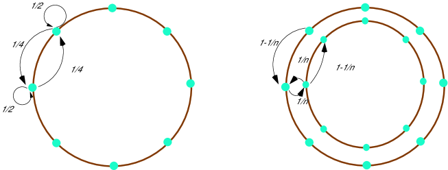
Figure 1:     (a) : $P_{1}$ on the ring graph $G_{1}$.                  (b) : $P_{2}$ on the lifted ring graph $G_{2}$.

In general, in most cases of interest the mixing time of the reversible walk $P$ scales like $1/\Phi^{2}(P)$. The conductance $\Phi(P)$ relates to diameter $D$ of a graph $G$ as $1/\Phi(P)\geq D$. Therefore, in such situations the mixing time of random walk based on the Metropolis-Hastings method is likely to scale like $D^{2}$, the square of the diameter. Indeed, Diaconis and Saloff-Coste [28] established that for a certain class of graphs with geometry the mixing time of any reversible random walk scales like at least $D^{2}$ and it is achieved by the Metropolis-Hastings’ approach. Thus, reversible random walks result in rather poor performance for graphs with geometry i.e. their mixing time is far from our best hope, the diameter $D$.

Motivated by this, we wish to undertake the following reasonably ambitious question in this paper: is it possible to design a random walk with mixing time of the order of diameter $D$ for any graph? We will answer this question in affirmative by producing a novel construction of non-reversible random walks on the lifted version of graph $G$. And thus, we will design iterative averaging algorithms with the fastest possible rate of convergence.

1.1 Related work

In an earlier work, Diaconis, Holmes and Neal [9] introduced a construction of a non-reversible random walk on the ring (and more generally ring-like) graph. This random walk runs on the lifted ring graph, which is described as $G_{2}$ in Figure 1(b). Here, by lifting we mean making additional copies of the nodes of the original graph and adding edges between some of these copies while preserving the original graph topology. Figure 1(b) explains the construction in [9] for the ring graph. Note that each node has two copies and the lifted graph is essentially composed of two rings: an inner ring and an outer ring. The transition on the inner circle forms a clockwise circulation and the transition on the outer circle forms a counterclockwise circulation. And the probability of changing from the inner circle to the outer circle and vice versa are $1/n$ each time. By defining transitions in this way, the stationary distribution is also preserved; i.e. the sum of stationary distributions of copies is equal to the stationary distribution of their original node. Somewhat surprisingly, the authors [9] proved that this non-reversible random walk has the linear mixing time $O^{*}(n)$. Thus, effectively (i.e. up to $\log n$ factor) the mixing time is of the order of the diameter $n$. It should be noted that because lifting preserves the graph topology and the stationary distribution, it is possible to simulate this lifted random walk on the original graph by expanding the state appropriately, with the desired output. Equivalently, it is possible to use a lifted random walk for linear averaging by running iterations with extra states.

The following question arose from the work of [9]: given graph $G$ and random walk $P$ on $G$, is it possible to design a non-reversible random walk on the lifted version of $G$ which mixes subsequently faster than $P$? Can it mix in $O(D)$? This question was addressed in a subsequent work by Chen, Lovász and Pak [7]. They provided an explicit construction of a random walk on a lifted version of $G$ with mixing time $O^{*}(1/\Phi(P))$. Further, they showed that, under the notion of lifting (implicity) introduced by [9] and formalized in [7], it is not possible to design such a lifted random walk with mixing time smaller than $\Omega(1/\Phi(P))$.

Now note that $1/\Phi(P)$ can be much larger than the diameter $D$. As a simple example, consider a ring graph with $P$ exactly the same as that in Figure 1(a), but with a difference that for two edges the transition probabilities are $\delta(n)$ instead of $1/4$ (and the transition probabilities of endpoints of these edges appropriately adjusted). Then, it can be checked that $1/\Phi(P)$ is $\Omega(n/\delta(n))$ which can be arbitrarily poor compared to the diameter $n$ by choosing small enough $\delta(n)$. A more interesting example showing this poorer scaling of $1/\Phi(P)$ compared to diameter, even for the Metropolis-Hastings’ style construction, is presented in Section 3 in the context of a “Barbell graph” (see Figure 2). Thus, the lifting approach of [9, 7] can not lead to a random walk with mixing time of the order of diameter and hence the question of existence or design of such a random walk remains unresolved.

As noted earlier, the lifted random walk can be used to design iterative algorithms (for computing an average) on the original graph since the topology of the lifted graph and the stationary distribution of the lifted random walk “projects back” onto those of the original graph and the random walk respectively. However, running algorithm based on lifted random walks on the original graph requires additional states. Specifically, the lifted random walk based algorithm can be simulated on the original graph by running multiple threads on each node. Specifically, the number of operations performed per iteration across the network depends on the size of the lifted walk (or graph). In the construction of [7] for a general graph, this issue about the size of the lifted walk was totally ignored as the authors’ interest was only the time complexity, not the size. Therefore, even though time may reduce under the construction of [7] the overall cost (equal to the product of time and size) may not be reduced; or even worse, it may increase.

Therefore, from the perspective of the application of iterative algorithms we need a notion of lifting that leads to a design of a random walk that has (a) mixing time of the order of diameter of the original graph and (b) the smallest possible size.

1.2 Our contributions

In this paper, we answer the above stated question affirmatively. As noted earlier, the notion of lifting of [9, 7] can not help in answering this question. For this reason, we introduce a notion of pseudo-lifting which can be thought of as a relaxation of the notion of lifting. Like lifting, the notion of pseudo-lifting preserves the topological constraints of the original graph. But the relaxation comes in preserving the stationary distribution in an approximate manner. However, it should be noted that is still possible to use the pseudo-lifted random walk to perform the iterative algorithm without any approximation errors (or to sample objects from a stationary distribution without any additional errors) since the stationary distribution of pseudo-lifting under a restricted projection provides the original stationary distribution exactly. Thus, operationally our notion of pseudo-lifting is as effective as lifting.

First, we use pseudo-lifting to design a random walk with mixing time of the order of diameter of a given graph with the desired stationary distribution. To achieve this, we first use the Metropolis-Hastings method to construct a random walk $P$ on the given graph $G$ with the desired stationary distribution. Then, we pseudo-lift this $P$ to obtain a random walk with mixing time of the order of diameter of $G$. This approach is stated as Theorem 5.

As discussed earlier, the utility of such constructions lies in the context of graphs with geometry. The graphs with (fixed) finite doubling dimension, introduced in [2, 13, 11, 8], serve as an excellent model for such a class of graphs. Roughly speaking, a graph has doubling dimension $\rho$ if the number of nodes within the shortest path distance $r$ of any node of $G$ is $O(r^{\rho})$ (i.e. polynomial growth of the neighborhood of a node). We apply our construction of pseudo-lifting to graphs with finite doubling dimension $\rho$ to obtain a random walk with mixing time of the order of diameter $D$. In order to address the concern with expansion in the size of the pseudo-lifted graph, we use the geometry of the original graph explicitly. Specifically, we reduce the size of the lifted graph by a clever combination of clustering, geometry and pseudo-lifting. This formal result is stated as follows and its proof is in Section 6.3.

Theorem 1.

Consider a connected graph $G$ with doubling dimension $\rho$ and diameter $D$. It is possible to explicitly construct a pseudo-lifted random walk on $G$ with mixing time $O(D)$ chain and size $O\left(Dn^{1-\frac{1}{1+\rho}}\right)$.

As a specific example, consider a $d$-dimensional grid whose doubling dimension is $d$. The Metropolis-Hastings method has mixing time $\Omega\left(n^{2/d}\right)$, compared to our construction with mixing time $O\left(n^{1/d}\right)$. Further, our construction leads to an increase in size of the random walk only by $O\left(n^{1/d(d+1)}\right)$ factor. That is, pseudo-lifting is optimal in terms of the number of iterations, which is equal to diameter, and in terms of cost per iteration it is lossy by a relatively small amount, for example $O\left(n^{1/d(d+1)}\right)$ for the $d$-dimensional grid.

In general, we can use pseudo-lifting to design iterative algorithms for computing the average of given numbers on the original graph itself. We describe a precise implementation of such an algorithm in Section 5. The use of pseudo-lifting, primarily effective for a class of graphs with geometry, results in the following formal result whose proof is in Section 5.2.

Theorem 2.

Consider a given connected graph $G$ with diameter $D$ and each node with a distinct value. Then, (using a pseudo-lifted random walk) it is possible to design an iterative algorithm whose $\varepsilon$-computation time is $T_{\varepsilon}=O^{*}\left(D\log\frac{1}{\varepsilon}\right)$. Further, if $G$ has doubling dimension $\rho$, then the network-wide total number of operations (essentially, additions) per iteration of the algorithm is $O\left(Dn^{1-\frac{1}{\rho+1}}\right)$.

As a specific example, recall a $d$-dimensional grid with doubling dimension $d$ and diameter $n^{1/d}$. The Metropolis-Hastings method will have mixing time $\Omega\left(n^{2/d}\right)$ and per iteration number of operations $\Theta(n)$. Therefore, the number of total operations is $O\left(n^{1+\frac{2}{d}}\right)$ (even the randomized gossip algorithm of [6] will have this total cost). Compared to this, Theorem 2 implies the number of iterations would be $O\left(n^{1/d}\right)$ and per iteration cost would be $O\left(n^{1+\frac{1}{d(d+1)}}\right)$. Therefore, the total cost is $O\left(n^{1+\frac{d+2}{d(d+1)}}\right)$ which is essentially close to $O\left(n^{1+1/d}\right)$ for large $d$. Thus, it strictly improves performance over the Metropolis-Hastings method by roughly $n^{1/d}$ factor. It is worth nothing that no algorithm can have the number of total operations less than $\Omega\left(n^{1+1/d}\right)$ and the number of iterations less than $\Omega\left(n^{1/d}\right)$.

For the application of interest of this paper, it was necessary to introduce a new notion of lifting and indeed we found one such notion, i.e. pseudo-lifting. In general, it is likely that for certain other applications such a notion may not exist. For this reason, we undertake the question of designing a lifted (not pseudo-lifted) random walk with the smallest possible size since the size (as well as the mixing time) decides the cost of the algorithm that uses lifting. Note that the average-computing algorithm in Section 5 can also be implemented via lifting instead of pseudo-lifting, and the size of lifting leads to the total number of operations. As the first step, we consider the construction of Chen, Lovász and Pak [7]. We find that it is rather lossy in its size. Roughly speaking, their construction tries to build a logical complete graph topology using the underlying graph structure. In order to construct one of $n^{2}$ edges of this complete graph topology, they use a solution of a flow optimization problem. This solution results in multiple paths between a pair of nodes. Thus, in principle, their approach can lead to a very large size. In order to reduce this size, we use two natural ideas: one, use a sparse expander graph instead of the complete graph and two, use a solution of unsplittable flows [19]. Intuitively, this approach seems reasonable but in order to make it work, we need to overcome rather non-trivial technical challenges. To address these challenges, we develop a method to analyze hybrid non-reversible random walks, which should be of interest in its own right. The formal result is stated as follows and see Section 6 for its complete proof.

Theorem 3.

Consider a given connected graph $G$ with a random walk $P$. Then, there exists a lifted random walk with mixing time $O^{*}(1/\Phi(P))$ and size $O^{*}(|E(P)|/\Phi(P))$, where

$$E(P)=\{(i,j):P_{ij}\neq 0~{}\mbox{or}~{}P_{ji}\neq 0\}.$$

Note that the lifted random walk in [7] has size $\Omega(n^{2}/\Phi(P))$, hence our lifting construction leads to the reduction of its size by $\Theta(n)$ factor when $G$ is sparse. Finally, we note that the methods developed for understanding the expander-based construction (and proof of Theorem 3) can be useful in making pseudo-lifting more robust, as discussed in the Section 7.

2 Preliminaries and Backgrounds

2.1 Key notions and definitions

In this paper, $G=(V,E)$ is a given graph with $n$ nodes i.e. $|V|=n$. We may use $V(G)$ to represent vertices of $V$ of $G$. $P$ always denotes a transition matrix of a graph conformant random walk (or Markov chain) on $G$ with its stationary distribution $\pi$ i.e. $P_{ij}>0$ only if $(i,j)\in E$, and $\pi^{T}P=\pi^{T}$. We will use the notion of “Markov chain” or “random walk” depending on which notion is more relevant to the context. The reverse chain $P^{*}$ of $P$ is defined as: $P^{*}_{ij}=\pi_{j}P_{ji}/\pi_{i}$ for all $(i,j)\in E$. We call $P$ reversible if $P=P^{*}$. Hence, if $\pi$ is uniform, $P$ is a symmetric matrix. The conductance of $P$ is defined as

$$\Phi(P)=\min_{S\subset V}\frac{\sum_{i\in S,j\in V\backslash S}\pi_{i}P_{ij}}{\pi(S)\pi(V\backslash S)},$$

where $\pi(A)=\sum_{i\in A}\pi_{i}$.

Although there are various (mostly equivalent) definitions of Mixing time that are considered in the literature based on different measures of the distance between distributions, we primarily consider the definition of Mixing time from the stopping rule. A stopping rule $\Gamma$ is a stopping time based on the random walk of $P$: at any time, it decides whether to stop or not, depending on the walk seen so far and possibly additional coin flips. Suppose, the starting node $w^{0}$ is drawn from distribution $\sigma$. The distribution of the stopping node $w^{\Gamma}$ is denoted by $\sigma^{\Gamma}=\tau$ and call $\Gamma$ as a stopping rule from $\sigma$ to $\tau$. Let $\mathcal{H}(\sigma,\tau)$ be the infimum of mean length over all such stopping rules from $\sigma$ to $\tau$. This is well-defined as there exists the following stopping rule from $\sigma$ to $\tau$: select $i$ with probability $\tau_{i}$ and walk until getting to $i$. Now, we present the definition of the (stopping rule based) Mixing time $\mathcal{H}$.

Definition 1 (Mixing time).

$\mathcal{H}=\max_{\sigma}\mathcal{H}(\sigma,\pi).$

Therefore, to bound $\mathcal{H}$, we need to design a stopping rule whose distribution of stopping nodes is $\pi$.

2.2 Metropolis-Hastings method

The Metropolis-Hastings method (or Glauber dynamics [18]) has been extensively studied in recent years due to its local constructibility. For a given graph $G=(V,E)$ and distribution $\pi$ on $V$, the goal is to produce a random walk $P$ on $G$ whose stationary distribution is $\pi$. The underlying idea of the random walk produced by this method is choosing a neighbor $j$ of the current vertex $i$ at uniformly random and moving to $j$ depending on the ratio between $\pi_{i}$ and $\pi_{j}$. Hence, its explicit transition matrix $P$ is following:

$$P_{ij}=\begin{cases}\frac{1}{2d}\min\{\frac{\pi_{j}}{\pi_{i}},1\}&\text{if }(i,j)\in E\\ 0&\text{if }(i,j)\notin E~{}\text{and }i\neq j\\ 1-\sum_{k\neq i}P_{ik}&\text{if }i=j\\ \end{cases},$$

where $d_{i}$ is a degree of vertex $i$ and $d=\max_{i}d_{i}$. It is easy to check that $\pi^{T}P=\pi^{T}$ and $P$ is reversible.

2.3 Lifting

As stated in the introduction, motivated by a simple ring example of Diaconis et al. [9], Chen et al. [7] use the following notion of lifting.

Definition 2 (Lifting).

A random walk $\widehat{P}$ on graph $\widehat{G}=(\widehat{V},\widehat{E})$ is called a lifting of random walk $P$ on graph $G=(V,E)$ if there exists a many-to-one function $f:\widehat{V}\to V$ such that the following holds: (a) for any $\widehat{u},\widehat{v}\in\widehat{V}$, $(\widehat{u},\widehat{v})\in\widehat{E}$ only if $(f(\widehat{u}),f(\widehat{v}))\in E$; (b) for any $u,v\in V$, $\pi(u)=\widehat{\pi}(f^{-1}(u))$ and $Q(u,v)=\widehat{Q}(f^{-1}(u),f^{-1}(v))$. Here $Q$ and $\widehat{Q}$ are ergodic flow matrices for $P$ and $\widehat{P}$ respectively.

Here, the ergodic flow matrix $Q=[Q_{ij}]$ of $P$ is defined as: $Q_{ij}=\pi_{i}P_{ij}$. It satisfies: $\sum_{i,j}Q_{ij}=1$, $\sum_{i}Q_{ij}=\sum_{i}Q_{ji}$ and $\sum_{i}Q_{ij}=\pi_{j}$. Conversely, every non-negative matrix $Q$ with these properties defines a random walk with the stationary distribution $\pi$. In this paper, $\widehat{P}$ means a lifted (or pseudo-lifted) random walk of $P$. Similarly $\widehat{G}$, $\widehat{V}$, $\widehat{E}$ and $\widehat{\pi}$ are the lifted (or pseudo-lifted) versions of their original one.

Chen et al. [7] provided an explicit construction to lift a given general random walk $P$ with almost optimal speed-up in terms of mixing time. Specifically, they obtained the following result.

Theorem 4 ([7]).

For a given random walk $P$, it is possible to explicitly construct a lifted random walk of $P$ with mixing time $O^{*}(1/\Phi(P))$. Furthermore, any lifted random walk of $P$ needs at least $\Omega(1/\Phi(P))$ time to mix.

2.4 Auxiliary backgrounds

2.4.1 $\varepsilon$-Mixing time

Here we introduce a different (and related) notion of Mixing time which measures more explicitly how fast the random walk converges to the stationarity. The following notions, $\tau(\varepsilon),\tau_{2}(\varepsilon)$ are related to ${\cal H}$. This relation can be found in detail in the survey by Lovász and Winkler [22]. For example, we will use this relation explicitly in Lemma 8.

Now we define these related definitions of mixing time. To this end, as before consider a random walk $P$ on a graph $G=(V,E)$. Let $P^{t}(x,\cdot)$ denote the distribution of the state after $t$ steps under $P$, starting from an initial state $x\in V$. For the random walk of our interest, $P^{t}(x,\cdot)$ goes to $\pi$ as $t\rightarrow\infty$. We present the definitions based on the total variation distance and the $\chi^{2}$-distance.

Definition 3 ($\varepsilon$-Mixing time).

Given $\varepsilon>0$, let $\tau(\varepsilon)$ and $\tau_{2}(\varepsilon)$ represent $\varepsilon$-Mixing time of the random walk with respect to the total variation distance and the $\chi^{2}$-distance respectively. Then, they are

$$\tau(\varepsilon)=\min\left\{t:\forall x\in V,\frac{1}{2}{\sum_{y\in\Omega}\left|P^{t}(x,y)-\pi(y)\right|}\leq\varepsilon\right\},$$

$$\tau_{2}(\varepsilon)=\min\left\{t:\forall x\in V,\sqrt{\sum_{y\in\Omega}\frac{1}{\pi(y)}\left(P^{t}(x,y)-\pi(y)\right)^{2}}\leq\varepsilon\right\}.$$

2.4.2 Additional Techniques to bound Mixing Times

Various techniques have been developed over past three decades or so to estimate Mixing time of a given random walk. The relation between the conductance and the mixing time in the introduction is one of them. We review some of the key other techniques that will be relevant for this paper.

Fill-up Lemma. Sometimes, due to the difficulty for designing such an exact stopping rule, we use the following strategy for bounding the mixing time $\mathcal{H}$.

• Step 1. For a positive constant $\varepsilon$ and any starting distribution $\sigma$, we design a stopping rule whose stopping distribution $\gamma$ is $\varepsilon$-far from $\pi$ (i.e. $\gamma\geq(1-\varepsilon)\pi$). This gives the upper bound for $H(\sigma,\gamma)$.

• Step 2. We bound $\mathcal{H}$ by $H(\sigma,\gamma)$ using the following fact known as fill-up Lemma in [1]:

  $$\mathcal{H}\leq\frac{1}{1-\varepsilon}\mathcal{H}_{\underline{\varepsilon}},$$

  where $\mathcal{H}_{\underline{\varepsilon}}=\max_{\sigma}\min_{\gamma\geq(1-\varepsilon)\pi}\mathcal{H}(\sigma,\gamma)$.

Eigenvalue. If $P$ is reversible, one can view $P$ as a self-adjoint operator on a suitable inner product space and this permits us to use the well-understood spectral theory of self-adjoint operators. It is well-known that $P$ has $n=|V|$ real eigenvalues $1=\lambda_{0}>\lambda_{1}\geq\lambda_{2}\geq\cdots\geq\lambda_{n-1}>-1$. The $\varepsilon$-mixing time $\tau_{2}(\varepsilon)$ is related as

$$\tau_{2}(\varepsilon)\leq\left\lceil\frac{1}{\lambda_{P}}\log\frac{1}{\varepsilon\sqrt{\pi_{0}}}\right\rceil,$$

where $\lambda_{P}=1-\max\{|\lambda_{1}|,|\lambda_{n-1}|\}$ and $\pi_{0}=\min_{i}\pi_{i}$. The $\lambda_{P}$ is also called the spectral gap of $P$. When $P$ is non-reversible, we consider $PP^{*}$. It is easy to see that the Markov chain with $PP^{*}$ as its transition matrix is reversible. Let $\lambda_{PP^{*}}$ be the spectral gap of this reversible Markov chain. Then, the mixing time of the original Markov chain (with its transition matrix $P$) is bounded above as:

$$\tau_{2}(\varepsilon)\leq\left\lceil\frac{2}{\lambda_{PP^{*}}}\log\frac{1}{\varepsilon\sqrt{\pi_{0}}}\right\rceil.$$ (2)

3 Pseudo-Lifting

Here our aim is to obtain a random walk with mixing time of the order of the diameter for a given graph $G$ and stationary distribution $\pi$. As explained in the introduction, the following approach based on lifting does not work for this aim: first obtain a random walk with the desired stationary distribution using the Metropolis-Hastings method, and then lift it using the method in [7].

For example, consider the Barbell graph $G$ as shown in Figure 2: two complete graphs of $n/2$ nodes connected by a single edge. And, suppose $\pi$ is uniform. Now, consider a random walk $P$ produced by the Metropolis-Hastings method: the next transition is uniform among all the neighbor for each node. For such a random walk, it is easy to check that $1/\Phi(P)=\Omega(n^{2})$ and $\mathcal{H}=\Omega(n^{4})$. Therefore, the mixing time of any lifting is at least $\Omega(n^{2})$. However, this random walk is ill-designed to begin with because $1/\Phi(P)$ can be decreased up to $O(n)$ by defining its random walk in another way (i.e. increasing the probability of its linkage edge, and adding self-loops to non-linkage nodes not to change its stationary distribution). $1/\Phi(P)$ is still far from the diameter $D=O(1)$ nevertheless. Hence, from Theorem 4, lifting cannot achieve $O(D)$-mixing.

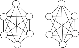
Figure 2: The Barbell graph with $12$ nodes.

Motivated by this limitation, we will use the following new notion of lifting, which we call pseudo-lifting, to design a $O(D)$-mixing random walk.

Definition 4 (Pseudo-Lifting).

A random walk $\widehat{P}$ is called a pseudo-lifting of $P$ if there exists a many-to-one function $f:\widehat{V}\to V$, $T\subset\widehat{V}$ with $|T|=|V|$ such that the following holds: (a) for any $\widehat{u},\widehat{v}\in\widehat{V}$, $(\widehat{u},\widehat{v})\in\widehat{E}$ only if $(f(\widehat{u}),f(\widehat{v}))\in E$, and (b) for any $u\in V$, $\widehat{\pi}(f^{-1}(u)\cap T)=\frac{1}{2}\pi(u).$

The property (a) in the definition implies that one can simulate the pseudo-lifting $\widehat{P}$ in the original graph $G$. Furthermore, the property (b) suggests that (by concentrating on the set $T$), it is possible to simulate the stationary distribution $\pi$ exactly via pseudo-lifting. Next we present its construction.

3.1 Construction

For a given random walk $P$, we will construct the pseudo-lifted random walk $\widehat{P}$ of $P$. It may be assumed that $P$ is given by the Metropolis-Hastings method. We will construct the pseudo-lifted graph $\widehat{G}$ by adding vertices and edges to $G$, and decide the values of the ergodic flows $\widehat{Q}$ on $\widehat{G}$, which defines its corresponding random walk $\widehat{P}$.

First, select an arbitrary node $v$. Now, for each $w\in V$, there exist paths $\mathcal{P}_{wv}$ and $\mathcal{P}_{vw}$, from $w$ to $v$ and $v$ to $w$ respectively. We will assume that all the paths are of length $D$: this can be achieved by repeating same nodes. Now, we construct a pseudo-lifted graph $\widehat{G}$ starting from $G$.

First, create a new node $v^{\prime}$ which is a copy of the chosen vertex $v$. Then, for every node $w$, add directed paths $\mathcal{P}^{\prime}_{wv}$, a copy of $\mathcal{P}_{wv}$, from $w$ to $v^{\prime}$. Similarly, add $\mathcal{P}^{\prime}_{vw}$ (a copy of $\mathcal{P}_{vw}$) from $v^{\prime}$ to $w$. Each addition creates $D-1$ new interior nodes. Thus, we have essentially created a virtual star topology using the paths of the old graph by adding $O(nD)$ new nodes in total. (Every new node is a copy of an old node.)

Now, we define the ergodic flow matrix $\widehat{Q}$ for this graph $\widehat{G}$ as follows: for an edge $(i,j)$,

$$\widehat{Q}_{ij}=\begin{cases}\frac{\delta_{1}}{2D}\pi_{w}\ \ &\text{if}\ (i,j)\in E(\mathcal{P}^{\prime}_{wv})\text{ or }E(\mathcal{P}^{\prime}_{vw})\\ (1-\delta_{1})Q_{ij}&\text{if}\ (i,j)\in E(G),\end{cases}$$

where $\delta_{1}\in[0.1]$ is a constant we will decide later in (3). It is easy to check that $\sum_{ij}\widehat{Q}_{ij}=1,\sum_{j}\widehat{Q}_{ij}=\sum_{j}\widehat{Q}_{ji}$. Hence it defines a a random walk on $\widehat{G}$. The stationary distribution of this pseudo-lifting is

$$\widehat{\pi}_{i}=\begin{cases}\frac{\delta_{1}}{2D}\pi_{w}\ \ &\text{if}\ i\in(V(\mathcal{P}^{\prime}_{wv})\cup V(\mathcal{P}^{\prime}_{vw}))\backslash\{w,v^{\prime}\}\\ \left(1-\delta_{1}+\frac{\delta_{1}}{2D}\right)\pi_{i}\ \ &\text{if}\ i\in V(G)\\ \frac{\delta_{1}}{2D}\ \ &\text{if}\ i=v^{\prime}\end{cases}$$

Given the above definition of $\widehat{Q}$ and corresponding stationary distribution $\widehat{\pi}$, it satisfies the requirements of pseudo-lifting in Definition 4 if we choose $\delta_{1}$ such that

$$1/2=\delta_{1}\left(1-\frac{1}{2D}\right),$$ (3)

and $T=V(G)$; i.e. $T$ is the set of old nodes.

3.2 Mixing time

We claim the following bound on the mixing time of the pseudo-lifting we constructed.

Theorem 5.

The mixing time of the random walk $\widehat{P}$ defined by $\widehat{Q}$ is $O(D)$.

Proof..

We will design a stopping rule where the distribution of the stopping node is $\widehat{\pi}$, and analyze its expected length. At first, walk until visiting $v^{\prime}$, and toss a coin $X$ with the following probability.

$$X=\begin{cases}0\ &\text{with probability}\ \frac{\delta_{1}}{2D}\\ 1\ \ &\text{with probability}\ \frac{\delta_{1}(D-1)}{2D}\\ 2\ \ &\text{with probability}\ 1-\delta_{1}+\frac{\delta_{1}}{2D}\\ 3\ \ &\text{with probability}\ \frac{\delta_{1}(D-1)}{2D}\\ \end{cases}$$

Depending on the value of $X$, the stopping node is decided as follows.

• $X=0$ : Stop at $v^{\prime}$. The probability for stopping at $v^{\prime}$ is $\Pr[X=0]=\frac{\delta_{1}}{2D}$, which is exactly $\widehat{\pi}_{v^{\prime}}$.

• $X=1$ : Walk a directed path $P^{\prime}_{vw}$, and choose an interior node of $P^{\prime}_{vw}$ uniformly at random, and stop there. For a given $w$, the probability for walking $P^{\prime}_{vw}$ is easy to check $\pi_{w}$. There are $D-1$ many interior nodes, hence, for an interior node $i$ of $P^{\prime}_{vw}$, the probability for stopping at $i$ is

  $$\Pr[X=1]\times\pi_{w}\times\frac{1}{D-1}=\frac{\delta_{1}}{2D}\pi_{w}=\widehat{\pi}_{i}.$$

• $X=2$ : Stop at the end node $w$ of $P^{\prime}_{vw}$. The probability for stopping at $w$ is

  $$\Pr[X=2]\times\Pr[\text{walk }P^{\prime}_{vw}]=\left(1-\delta_{1}+\frac{\delta_{1}}{2D}\right)\times\pi_{w}=\widehat{\pi}_{w}.$$

• $X=3$ : Walk until getting a directed path $P^{\prime}_{wv}$, and choose an interior node of $P^{\prime}_{wv}$ uniformly at random, and stop there. Until getting a directed path $P^{\prime}_{wv}$, the pseudo-lifted random walk defined by $\widehat{Q}$ is same as the original random walk. Since the distribution $w\in V(G)$ of the walk at the end of the previous step is exactly $\pi$, it follows that the distribution $\pi$ over the nodes of $V(G)$ is preserved under this walk till walking on $P^{\prime}_{wv}$. From the same calculation as the case $X=1$, the probability of stopping at the interior node $i$ of $P^{\prime}_{wv}$ is $\widehat{\pi}_{i}$.

Therefore, we have established the existence of a stopping rule that takes an arbitrary starting distribution to the stationary distribution $\widehat{\pi}$. Now, this stopping rule has an average length $O(D/\delta_{1})$: since the probability of getting on a directed path $P^{\prime}_{wv}$ at $w$ is $\frac{\delta_{1}}{2D}/(1-\delta_{1}+\frac{\delta_{1}}{2D})=\Theta(\delta_{1}/D)$, the expected numbers of walks until visiting $v^{\prime}$ and getting a directed path when $X=3$ are $O(D/\delta_{1})=O(D)$ from (3) in both cases. This completes the proof. $\Box$

4 Pseudo-Lifting: use of geometry

The graph topologies arising in practice, such as those in wireless sensor network deployed in some geographic area or a nearest neighbor network of unmanned vehicles [30], do possess geometry and are far from being expanders. A good model for graphs with geometry is a class of graphs with finite doubling dimension which is defined as follows.

Definition 5 (Doubling Dimension).

Consider a metric space $\mathcal{M}=(\mathcal{X},\mathbf{d})$, where $\mathcal{X}$ is the set of point endowed with a metric $\mathbf{d}$. Given $x\in\mathcal{X}$, define a ball of radius $r\in\mathbb{R}_{+}$ around $x$ as $\mathbf{B}(x,r)=\{y\in\mathcal{X}:\mathbf{d}(x,y)<r\}$. Define

$$\rho(x,r)=\inf\{K\in\mathbb{N}:\exists~{}y_{1},\dots,y_{K}\in\mathcal{X},\mathbf{B}(x,r)\subset\cup_{i=1}^{K}\mathbf{B}(y_{i},r/2)\}.$$

Then, the $\rho(\mathcal{M})=\sup_{x\in\mathcal{X},r\in\mathbb{R}_{+}}\rho(x,r)$ is called the doubling constant of $\mathcal{M}$ and $\log_{2}\rho(\mathcal{M})$ is called the doubling dimension of $\mathcal{M}$. The doubling dimension of a graph $G=(V,E)$ is defined with respect to the metric induced on $V$ by the shortest path metric.

For graphs with finite doubling dimension, we will design a pseudo-lifting with its efficient size. Recall the basic idea for the construction of the pseudo-lifting in Section 3 is creating a virtual star topology using paths from every node to a fixed root, and the length of paths grows the size of the pseudo-lifting. To reduce the overall length of paths, we consider clusters of nodes such that nodes in each cluster are close to each other, and pick a sub-root node in each cluster. And then, build a star topology in each cluster around its sub-root and connect every sub-root to the root. This creates a hierarchical star topology (or say a tree topology) as you see the example of the line graph in Figure 3(b). Since it needs paths of short length in each cluster, the overall length of paths would be decreased.

For a good clustering, we need to decide which nodes would become sub-roots. A natural candidate for them is the $R$-net $Y\subset V$ of a graph $G$ defined as follows.

Definition 6 ($R$-net).

For a given graph $G=(V,E)$, $Y\subset V$ is a $R$-net if

• For every $v\in V$, there exists $u\in Y$ such that the shortest path distance between $u,v$ is at most $R$.

• The distance between any two $y,z\in Y$ is more than $R$.

Such an $R$-net can be found in $G$ greedily, and as you will see the proof of Lemma 7, the small doubling dimension of $G$ guarantees the existence of a good $R$-net for our purpose.

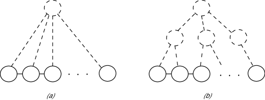
Figure 3: For a given line graph with $n$ nodes, (a) is the star topology which used in the construction of the pseudo-lifted graph in Section 3.1. (b) is the hierarchical star topology which will be used in this section for the new construction of pseudo-lifting.

4.1 Construction

For a given random walk $P$, we will construct the pseudo-lifted random walk $\widehat{P}$ of $P$ using a hierarchical star topology. Denote $\pi$ and $G=(V,E)$ be the stationary distribution and the underlying graph of $P$ again. As the previous construction in Section 3.1, we will construct the pseudo-lifted graph $\widehat{G}$ by extending $G$, and define the ergodic flow matrix $\widehat{Q}$ on $\widehat{G}$, which leads to its corresponding random walk $\widehat{P}$.

Given a $R$-net $Y$, match each node $w$ to the nearest $y\in Y$ (breaking ties arbitrarily). Let $C_{y}=\{w|\ w$ matched to $y\}$ for $y\in Y$. Clearly, $V=\cup_{y\in Y}C_{y}$. Finally, for each $y\in Y$ and for any $w\in C_{y}$ we have paths $\mathcal{P}_{wy},\mathcal{P}_{yw}$ between $w$ and $y$ of length $R$ exactly. Also, for each $y\in Y$, there exit $\mathcal{P}_{yv},\mathcal{P}_{vy}$ between $y$ and $v$ of length $D$ exactly (we allow the repetition of nodes to hit this length exactly).

Now, we construct the pseudo-lifted graph $\widehat{G}$. As the construction in Section 3.1, select an arbitrary node $v\in V$ and create its copy $v^{\prime}$ again. Further, for each $y\in Y$, create two copies $y_{1}^{\prime}$ and $y_{2}^{\prime}$. Now, add directed paths $\mathcal{P}^{\prime}_{wy}$, a copy of $\mathcal{P}_{wy}$, from $w$ to $y^{\prime}_{1}$ and add $\mathcal{P}^{\prime}_{yv}$, a copy of $\mathcal{P}_{yv}$, from $y^{\prime}_{1}$ to $v^{\prime}$. Similarly, add $\mathcal{P}^{\prime}_{vy}$ and $\mathcal{P}^{\prime}_{yw}$ between $v^{\prime}$, $y^{\prime}_{2}$ and $y^{\prime}_{2}$, $w$. In total, this construction for $\widehat{G}$ adds $2D|Y|+2Rn$ edges to $G$. Now, the ergodic flow matrix $\widehat{Q}$ on $\widehat{G}$ is defined as follows: for any $(i,j)$ of $\widehat{G}$,

$$\widehat{Q}_{ij}=\begin{cases}\frac{\delta_{2}}{2(R+D)}\pi_{w}\ \ &\text{if}\ (i,j)\in E(\mathcal{P}^{\prime}_{wy})\text{ or }E(\mathcal{P}^{\prime}_{yw})\\ \frac{\delta_{2}}{2(R+D)}\pi(C_{y})\ \ &\text{if}\ (i,j)\in E(\mathcal{P}^{\prime}_{yv})\text{ or }E(\mathcal{P}^{\prime}_{vy})\\ (1-\delta_{2})Q_{ij}&\text{if}\ (i,j)\in E(G)\end{cases},$$

where $\pi(C_{y})=\sum_{w\in C_{y}}\pi_{w}$ and $\delta_{2}\in[0.1]$ is a constant decided later. It can be checked that $\sum_{ij}\widehat{Q}_{ij}=1,\sum_{j}\widehat{Q}_{ij}=\sum_{j}\widehat{Q}_{ji}$. Hence it defines a random walk on $\widehat{G}$. The stationary distribution of this pseudo-lifted chain is

$$\widehat{\pi}_{i}=\begin{cases}\frac{\delta_{2}}{2(R+D)}\pi_{w}\ \ &\text{if}\ i\in(V(\mathcal{P}^{\prime}_{wy})\cup V(\mathcal{P}^{\prime}_{yw}))\backslash\{w,y^{\prime}_{1},y^{\prime}_{2}\}\\ \frac{\delta_{2}}{2(R+D)}\pi(C_{y})\ \ &\text{if}\ i\in(V(\mathcal{P}^{\prime}_{yv})\cup V(\mathcal{P}^{\prime}_{vy}))\backslash\{v^{\prime}\}\\ \left(1-\delta_{2}(1-\frac{\delta_{2}}{2(R+D)})\right)\pi_{i}\ \ &\text{if}\ i\in V(G)\\ \frac{\delta_{2}}{2(R+D)}\ \ &\text{if}\ i=v^{\prime}\end{cases}$$

To guarantee that this chain is indeed the pseudo-lifting of the original random walk $P$, consider $T=V(G)$ and $\delta_{2}$, where

$$\frac{1}{2}=\delta_{2}\left(1-\frac{1}{2(R+D)}\right).$$ (4)

Note that $\widehat{G}$ has exactly $|E|+2Rn+2D|Y|$ edges.

4.2 Mixing time and Size: Proof of Theorem 1

We prove two Lemmas about the performance of pseudo-lifting we constructed, and they imply Theorem 1. At first, we state the following result about its mixing time, and the proof can be done similarly as the proof of Theorem 5.

Lemma 6.

The mixing time of the random walk $\widehat{P}$ defined by $\widehat{Q}$ is $O(D)$.

Proof..

Consider the following stopping rule. Walk until visiting $v^{\prime}$, and toss a coin $X$ with the following probability.

$$X=\begin{cases}0\ &\text{with probability}\ \frac{\delta_{2}}{2(R+D)}\\ 1\ \ &\text{with probability}\ \frac{\delta_{2}D}{2(R+D)}\\ 2\ \ &\text{with probability}\ \frac{\delta_{2}(R-1)}{2(R+D)}\\ 3\ \ &\text{with probability}\ 1-\delta_{2}(1-\frac{\delta_{2}}{2(R+D)})\\ 4\ \ &\text{with probability}\ \frac{\delta_{2}(R-1)}{2(R+D)}\\ 5\ \ &\text{with probability}\ \frac{\delta_{2}D}{2(R+D)}\\ \end{cases}$$

Depending on the value of $X$,

• $X=0$ : Stop at $v^{\prime}$.

• $X=1$ : Walk on a directed path $\mathcal{P}^{\prime}_{vy}$, and choose its interior node uniformly at random, and stop there.

• $X=2$ : Walk until getting a directed path $\mathcal{P}^{\prime}_{yw}$, and choose its interior node uniformly at random, and stop there.

• $X=3$ : Walk until getting an old node in $V(G)$, and stop there.

• $X=4$ : Walk until getting a directed path $\mathcal{P}^{\prime}_{wy}$, and choose its interior node uniformly at random, and stop there.

• $X=5$ : Walk until getting a directed path $\mathcal{P}^{\prime}_{yv}$, and choose its interior node uniformly at random, and stop there.

It can be checked, using arguments similar to that in proof of Theorem 5, that the distribution of the stopped node is precisely $\widehat{\pi}$. Also, we can show that the expected length of this stopping rule is $O(\frac{R+D}{\delta}_{2})=O(\frac{D}{\delta}_{2})=O(D)$ from (4). This is primarily true because the probability of getting on a directed path $\mathcal{P}^{\prime}_{wy}$ at $w$ is $\Theta(\delta_{2}/(R+D))$. $\Box$

Now we apply the hierarchical construction to the case of graphs with constant doubling dimension, and show the guarantee for the size of the pseudo-lifting in terms of its doubling dimension.

Lemma 7.

Given a graph $G$ with a constant doubling dimension $\rho$ and its diameter $D$, the hierarchical construction gives a pseudo-lifted graph $\widehat{G}$ with its size $|\widehat{E}|=O(Dn^{1-\frac{1}{\rho+1}})$.

Proof..

The property of doubling dimension graph implies that there exists an $R$-net $Y$ such that $|Y|\leq(2D/R)^{\rho}$ (cf. [2]). Consider $R=D2^{\frac{\rho}{\rho+1}}n^{-\frac{1}{\rho+1}}$. This is an appropriate choice because $R=D2^{\frac{\rho}{\rho+1}}n^{-\frac{1}{\rho+1}}>Dn^{-\frac{1}{\rho+1}}>n^{\frac{1}{\rho}-\frac{1}{\rho+1}}>1$ (the second inequality is from $n\leq D^{\rho}$). Given this, the size of the pseudo-lifted graph $\widehat{G}$ is

$$|\widehat{E}|=|E|+2Rn+2D|Y|\leq|E|+2D\left(\frac{2^{\frac{\rho}{\rho+1}}}{n^{\frac{1}{\rho+1}}}\right)n+2D\left(2\frac{n^{\frac{1}{\rho+1}}}{2^{\frac{\rho}{\rho+1}}}\right)^{\rho}=|E|+O(Dn^{1-\frac{1}{\rho+1}}).$$

Since $|E|=O(n)$ and $D=\Omega(n^{1/\rho})$, we have that $|\widehat{E}|=O(Dn^{1-\frac{1}{\rho+1}})$. $\Box$

5 Application: Back to Averaging

As we introduced in the introduction, consider the following computation problem of the distributed averaging. Given a connected network graph $G=(V,E)$, where $V=\{1,2,\ldots n\}$, each node $i\in V$ has a value $x_{i}\in\mathbb{R}$. Then the goal is to compute the average of $\mathbf{x}=[x_{i}]$ only by communications between adjacent nodes:

$$x_{ave}=\frac{1}{n}\sum_{i}x_{i}.$$ (5)

This problem arises in many applications such as distributed estimation [31], distributed spectral decomposition [17], estimation and distributed data fusion on ad-hoc networks [23], distributed sub-gradient method for eigenvalue maximization [5], inference in Gaussian graphical models [24], and coordination of autonomous agents [15].

5.1 Linear iterative algorithm

A popular and quite simple approach for this computation is a method based on linear iterations [32] as follows. Suppose we are given with a graph conformant random walk $P$ which has the uniform stationary distribution $\pi$ i.e. $\pi^{T}P=\pi^{T}$. The linear iteration algorithm is described as follows. At time $t$, each node $i\in V$ has an estimate $y_{i}(t)$ of $x_{ave}$ and initially $y_{i}(0)=x_{i}$. At time $t=1,2,\ldots$ for each edge $(i,j)$ of $G$, node $i$ sends value $P_{ji}y_{i}(t)$ to node $j$. Then each node $j$ sums up the values received as its estimate at time $t+1$, that is

$$y_{j}(t+1)=\sum_{i=1}^{n}P_{ji}y_{i}(t).$$

Under the condition that $P$ is ergodic, i.e. $P$ is connected and aperiodic, it is known that [32]

$$\lim_{t\rightarrow\infty}y(t)=\lim_{t\rightarrow\infty}P^{t}\mathbf{x}=\left(\sum_{i}x_{i}\right)\pi=\frac{1}{n}\sum_{i}x_{i}\mathbf{1}=x_{ave}\mathbf{1},~{}\mbox{where}~{}\mathbf{1}=[1].$$

Specifically, as we already saw in the introduction, $\varepsilon$-computation time $T_{\varepsilon}(P)$ is defined as:

$$T_{\varepsilon}(P) = \inf\left\{t~{}:~{}\forall\mathbf{x}\in\mathbb{R}_{+}^{n},\frac{\|P^{t}\mathbf{x}-x_{ave}\mathbf{1}\|_{\infty}}{x_{ave}}\leq\varepsilon\right\}.$$ (6)

The quantity $T_{\varepsilon}(P)$ is well known to be related to the mixing time $\mathcal{H}(P)$. More precisely, we prove Lemma 8, which implies

$$T_{\varepsilon}(P)=O^{*}\left(\mathcal{H}(P)\log\frac{1}{\varepsilon}\right).$$ (7)

Since each edge $(i,j)$ such that $P_{ij}>0$ performs an exchange of values per each iteration, the number of operations performed per iteration across the network is at most $|E|$. Thus, the total number of operations of the linear iterations to obtain the approximation of $x_{ave}$ scales like

$$C_{\varepsilon}(P):=T_{\varepsilon}(P)\times|E|.$$ (8)

Therefore, the task of designing an appropriate $P$ with small $\mathcal{H}(P)$ is important to minimize both $T_{\varepsilon}(P)$ and $C_{\varepsilon}(P)$.

5.2 Linear iterative algorithm with pseudo-lifting: Proof of Theorem 2

We present a linear iterative algorithm that utilizes the pseudo-lifted version of a given matrix $P$ on the original graph $G$. The main idea behind this implementation is to run the standard linear iterations in $\widehat{G}=(\widehat{V},\widehat{E})$ with the pseudo-lifted chain $\widehat{P}$. However, we wish to implement this on $G=(V,E)$ and not $\widehat{G}$. Now recall that $\widehat{G}$ has the following property: (a) each node $\widehat{v}\in\widehat{V}$ is a copy of a node $v\in V$, and (b) each edge $(\widehat{u},\widehat{v})$ is a copy of edge $(u,v)\in E$, where $\widehat{u},\widehat{v}$ are copies of $u,v\in V$ respectively. Therefore, each node $\widehat{v}\in V$ can be simulated by a node $v\in V$ where $\widehat{v}$ is a copy of $v$ for the purpose of linear iterations. Thus, it is indeed possible to simulate the pseudo-lifted version of a matrix $P$ on $G$ by running multiple threads (in the language of the computer programming) on each node of $G$. We state this approach formally as follows:

• Given graph $G=(V,E)$, we wish to compute the average $x_{ave}$ at all nodes. For this, first produce a matrix $P$ using the Metropolis-Hastings method with the uniform stationary distribution.

• Construct the pseudo-lifting $\widehat{P}$ based on $P$ as explained in Section 4. This pseudo-lifted random walk has a stationary distribution $\widehat{\pi}$ on a graph $\widehat{G}$.

• As explained below, implement the linear iterative algorithm based on $\widehat{P}$ on the original graph $G$.

  • Let $t$ be the index of iterations of the algorithm and initially it be equal to $0$.

  • For each node $\widehat{v}\in\widehat{V}$, maintain a number $y_{\widehat{v}}(t)$ at the $t^{th}$ iteration. This is maintained at the node $v\in V$ where $\widehat{v}$ is a copy of $v$. The initialization of these values is stated below.

    • Recall that, $\widehat{V}$ contains $V$ as its subset. Recall that they are denoted as $V(G)\subset\widehat{V}$, and each $v\in G$ has its copy $\bar{v}\in V(G)$.

    • For each $\widehat{v}\in V(G)$, initialize $y_{\widehat{v}}(0)=x_{v}$.

    • For each $\widehat{v}\in V\backslash V(G)$, initialize $y_{\widehat{v}}(0)=0$.

  • In the $t+1^{th}$ iteration, update

    $$y_{\widehat{v}}(t+1)=\sum_{\widehat{u}\in\widehat{V}}\widehat{P}_{\widehat{v}\widehat{u}}y_{\widehat{u}}(t).$$

    This update is performed by each node $v$ through receiving information from its neighbors $u$ in $G$, where $\widehat{v}$ is a copy of $v$ and neighbors (of $\widehat{v}$) $\widehat{u}$ are copies of neighbors (of $v$) $u$.

• At the end of the $t^{th}$ iteration, each node $v$ produces its estimate as $2y_{\widehat{v}}(t)$, $\widehat{v}\in V(G)$.

It can be easily verified that since above algorithm is indeed implementing the linear iterative algorithm based on $\widehat{P}$, the $\varepsilon$ computation time is $T_{\varepsilon}(\widehat{P})$ and the total number of communications performed is $C_{\varepsilon}(\widehat{P})$. In what follows, for the completeness we bound $T_{\varepsilon}(\widehat{P})$ and $C_{\varepsilon}(\widehat{P})$.

Lemma 8.

$T_{\varepsilon}(\widehat{P})=O\left(\mathcal{H}(\widehat{P})\log\frac{1}{\varepsilon\pi_{0}}\right)$.

Proof..

Here, we need the $\varepsilon$-mixing time $\tau(\varepsilon)$ based on the total variance distance, and recall its definition in Section 2.4:

$$\tau(\varepsilon)=\min\left\{t:\forall i\in G,\frac{1}{2}{\sum_{j\in G}\left|P^{t}_{ij}-\pi_{j}\right|}\leq\varepsilon\right\}.$$

The following relation between two different mixing time $\tau(\varepsilon)$ and $\mathcal{H}$ is known (see [22]):

$$\tau(\varepsilon)=O\left(\mathcal{H}\log{\frac{1}{\varepsilon}}\right).$$

If $t$ is larger than $\tau(\varepsilon\pi_{0}/4)$ of $\widehat{P}$ , which is $O\left(\mathcal{H}(\widehat{P})\log\frac{1}{\varepsilon\pi_{0}/4}\right)$,

$$\left|y_{i}(t)-\langle y(0),\widehat{\pi}\rangle\right| = \left|\sum_{j}\widehat{P}^{t}_{ij}y_{j}(0)-\sum_{j}y_{j}(0)\widehat{\pi}_{j}\right|~{}\leq~{}\sum_{j}y_{j}(0)\left|\widehat{P}^{t}_{ij}-\widehat{\pi}_{j}\right|$$

$$\stackrel{{\scriptstyle(a)}}{{\leq}} \sum_{j}y_{j}(0)\frac{\varepsilon\pi_{0}}{2}~{}\stackrel{{\scriptstyle(b)}}{{\leq}}~{}\sum_{j}y_{j}(0)\varepsilon\widehat{\pi}_{j}~{}=~{}\varepsilon\langle y(0),\widehat{\pi}\rangle,$$

where (a) is from $\left|\widehat{P}^{t}_{ij}-\widehat{\pi}_{j}\right|\leq\sum_{j}\left|\widehat{P}^{t}_{ij}-\widehat{\pi}_{j}\right|\leq 2\times\frac{\varepsilon\pi_{0}}{4}=\frac{\varepsilon\pi_{0}}{2}$, and (b) is because $\widehat{\pi}_{j}>\frac{1}{2}\pi_{j}\geq\frac{1}{2}\pi_{0}$ for every old node $j\in V(G)$, and $y_{j}(0)=0$ otherwise. This completes the proof. $\Box$

From the proof of Lemma 8, note that the relation $T_{\varepsilon}(P)=O\left(\mathcal{H}(P)\log\frac{1}{\varepsilon\pi_{0}}\right)$ holds for any random walk $P$. Therefore, $T_{\varepsilon}(\widehat{P})=O\left(D\log\frac{1}{\varepsilon\pi_{0}}\right)$ and $C_{\varepsilon}(\widehat{P})=T_{\varepsilon}(\widehat{P})\times|\widehat{E}|=O\left(D^{2}n^{1-\frac{1}{1+\rho}}\log\frac{1}{\varepsilon\pi_{0}}\right)$ since $\mathcal{H}(\widehat{P})=O(D)$ and $|\widehat{E}|=O(Dn^{1-\frac{1}{1+\rho}})$ from Lemma 6 and 7. This also completes the proof of Theorem 2.

5.3 Comparison with other algorithms

Even considering any possible algorithms based on passing messages, the lower bound of the performance guarantees in the averaging problem is $O(D)$ for the running time, and $O(Dn)$ for the total number of operations. Therefore, our algorithm using pseudo-lifting gives the best running time, and possibly loses $\frac{O^{*}(D^{2}n^{1-\frac{1}{\rho+1}})}{O(Dn)}=O^{*}(D/n^{\frac{1}{\rho+1}})$ factor in terms of the total number of operations compared to the best algorithm. For example, when $G$ is a $d$-dimensional grid graph, this loss is only $O^{*}(D/n^{\frac{1}{\rho+1}})=O^{*}(n^{1/d}/n^{\frac{1}{d+1}})=O^{*}(n^{\frac{1}{d(d+1)}})$ since the doubling dimension of $G$ is $d$ and its diameter $D$ is $O(n^{1/d})$. The standard linear iterations using the Metropolis-Hastings method loses $\Omega(n^{1/d})$ factor in both the running time and the total number of operations (see Table I).

	Metropolis-Hastings	Pseudo-Lifting	Optimal
$\mathop{\mbox{Mixing time(Running time)}}\limits_{:~{}d\mbox{-dim. grid graph}}$	$\mathop{\Omega\left(\frac{1}{\Phi^{2}(P)}\right)}\limits_{:~{}O^{*}\left(n^{\frac{2}{d}}\right)}$	$\mathop{O(D)}\limits_{:~{}O\left(n^{\frac{1}{d}}\right)}$	$\mathop{D}\limits_{:~{}n^{\frac{1}{d}}}$
$\mathop{\mbox{Size (dbl. dim. $\rho$)}}\limits_{:~{}d\mbox{-dim. grid graph}}$	$\mathop{\Theta(n)}\limits_{:\Theta(n)}$	$\mathop{O\left(n^{\frac{\rho}{\rho+1}}D\right)}\limits_{:~{}O\left(n^{1+\frac{1}{d(d+1)}}\right)}$	$\mathop{n}\limits_{:~{}n}$
$\mathop{\mbox{Total }\#\mbox{ of operations}}\limits_{:~{}d\mbox{-dim. grid graph}}$	$\mathop{\Omega\left(\frac{n}{\Phi^{2}(P)}\right)}\limits_{:~{}O^{*}\left(n^{1+\frac{2}{d}}\right)}$	$\mathop{O\left(n^{\frac{\rho}{\rho+1}}D^{2}\right)}\limits_{:~{}O^{*}\left(n^{1+\frac{d+2}{d(d+1)}}\right)}$	$\mathop{nD}\limits_{:~{}n^{1+\frac{1}{d}}}$

Table 1: Comparison of pseudo-lifting with the Metropolis-Hastings method. Here, we assume $G$ has $\Theta(n)$ edges.

We take note of the following subtle matter: the non-reversibility is captured in the transition probabilities of the underlying Markov chain (or random walk); but the linear iterative algorithm does not change its form other than this detail.

6 Lifting Using Expanders

We introduced the new notion of pseudo-lifting for the applications of interest, one of which was the distributed averaging. However, since it may not be relevant to certain other applications, we optimize the size of lifting (not pseudo-lifting) in [7]. The basic motivation of our construction is using the expander graph, instead of the complete graph in [7], to reduce the size of the lifting.

6.1 Preliminaries

In what follows, we will consider only $P$ such that $P\geq I/2$. This is without loss of generality due to the following reason. Suppose such is not the case, then we can modify it as $(I+P)/2$; the mixing time of $(I+P)/2$ is within a constant factor of the mixing time of $P$.

6.1.1 Multi-commodity Flows

In [7], the authors use a multi-commodity flow to construct a specific lifting of a given random walk $P$ to speed-up its mixing time. Specifically, they consider a multi-commodity flow problem on $G$ with the capacity constraint on edge $(u,v)\in E$ given by $Q_{uv}$. A flow from a source $s$ to a destination $t$, denoted by $f$, is defined as a non-negative function on edges of $G$ so that

$$\sum_{j}f(ji)=\sum_{j}f(ij)$$

for every node $i\neq s,t$. The value of the flow is defined by

$$val(f)=\sum_{j}f(sj)-\sum_{j}f(js)=\sum_{j}f(jt)-\sum_{j}f(tj)$$

, and the cost of flow $f^{st}$ is defined as

$$cost(f)=\sum_{(i,j)\in E}f(ij).$$

A multi-commodity flow is a collection $f=(f^{st})$ of flows, where each $f^{st}$ is a flow from $s$ to $t$. Define the congestion of a multi-commodity flow $f$ as

$$\max_{(i,j)\in E}\frac{\sum_{s,t}f^{st}(ij)}{Q_{ij}}.$$

Consider the following optimization problem, essentially trying to minimize the congestion and the cost simultaneously under the condition for the amount of flows:

$${\sf minimize}~{}~{}~{}~{}K$$

$${\sf subject~{}to}~{}~{}val(f^{st})=\pi_{s}\pi_{t},~{}~{}\forall s,t,$$

$$~{}~{}~{}~{}~{}~{}~{}~{}~{}~{}~{}~{}~{}~{}\sum_{s,t}f^{st}(ij)\leq KQ_{ij},~{}~{}\forall(i,j)\in E,$$

$$~{}~{}~{}~{}~{}~{}~{}~{}~{}~{}~{}~{}~{}~{}\sum_{t}cost(f^{st})\leq K\pi_{s},~{}\sum_{s}cost(f^{st})\leq K\pi_{t},~{}\forall s,t.$$

Let $C$ be the optimal solution of the above problem. It is easy to see that $C\geq 1/\Phi$. Further, if $P$ is reversible, then result of Leighton and Rao [21] on the approximate multi-commodity implies that

$$C=O\left(\frac{1}{\Phi}\log\frac{1}{\pi_{0}}\right).$$

Let the optimal multi-commodity flow of the above problem be $F_{1}$, and we can think of $F_{1}$ as a weighted collection of directed paths. In [7], the authors modified $F_{1}$, and got a new multi-commodity flow $F_{2}$ that has the same amount of $s-t$ flows as $F_{1}$, while its congestion and path length are at most $12C$. They used $F_{2}$ to construct a lifting $\widehat{P}$ with mixing time $\widehat{\mathcal{H}}$ such that

$$\widehat{\mathcal{H}}\leq 144C.$$

Also, they showed that the mixing time of any lifting $\widehat{P}$ is greater than $C/2$, hence their lifted Markov chain has almost optimal speed-up within a constant factor.

To obtain a lifting with the smaller size than that in [7], we will to study the existence of the specific $k$-commodity flow with short path lengths. For this, we will use a balanced multi-commodity flow, which is a multi-commodity flow with the following condition for the amount of flows:

$$val(f^{st})=g(s,t),\forall s,t,$$

and $g(s,t)$ satisfies the balanced condition:

$$\sum_{t}g(s,t)\leq\pi_{s},~{}\sum_{s}g(s,t)\leq\pi_{t},~{}~{}\forall s,t.$$

Therefore, $F_{1}$ and $F_{2}$ are also balanced multi-commodity flows with $g(s,t)=\pi_{s}\pi_{t}$. Given a multi-commodity flow $f$, let $C(f)$ be its congestion and $D(f)$ be the length of the longest flow-path. Then, the flow number $T$ is defined follows:

$$T=\min_{f}\left(\max\left\{C(f),D(f)\right\}\right),$$

where the minimum is taken over all balanced multi-commodity flows with $g(s,t)=\pi_{s}\pi_{t}$. Hence, $F_{2}$ implies $T\leq 12C$. The following claim appears in [19]:

Claim 9.

(Claim 2.2 in [19]) For any $g(s,t)$ satisfying the balanced condition (not necessarily $g(s,t)=\pi_{s}\pi_{t}$), there exists a balanced multi-commodity flow $f$ with $g(s,t)$ such that $\max\{C(f),D(f)\}\leq 2T$.

6.1.2 Expanders

The expander graphs are sparse graphs which have high connectivity properties, quantified using the edge expansion $h(G)$ as defined as

$$h(G)=\min_{1\leq|S|\leq\frac{n}{2}}\frac{|\partial(S)|}{|S|},$$

where $\partial(S)$ is the set of edges with exactly one endpoint in $S$. For constants $d$ and $c$, a family $\mathcal{G}=\{G_{1},G_{2},\dots\}$ of $d$-regular graphs is called a $(d,c)$-expander family if $h(G)>c$ for every $G\in\mathcal{G}$. There are many explicit constructions of a $(d,c)$-expander family available in recent times. We will use a $(d,c)$-expander graph $G^{Ex}=(V,E^{Ex})$ (i.e. $V^{Ex}=V$), and a transition matrix $P^{Ex}$ defined on this graph. For a given $\pi$, we can define a reversible $P^{Ex}$ so that its stationary distribution is $\pi$ as follows,

$$P^{Ex}_{ij}=\begin{cases}\frac{\pi_{0}}{d\pi_{i}}&\text{if }(i,j)\in E^{Ex}\\ 1-\frac{\pi_{0}}{\pi_{i}}&\text{if }i=j\\ \end{cases}.$$

In the case of $\pi_{max}=O(\pi_{0})$, it is easy to check that $\Phi(P^{Ex})=\Theta(h(G))=\Omega(1)$, where $\Phi(P^{Ex})$ is the conductance of $P^{Ex}$. Hence, $\lambda_{P^{Ex}}=\Omega(1)$, and the random walk defined by $P^{Ex}$ mixes fast. In this Section, we will consider only such $\pi$.

6.2 Construction

We use the multi-commodity flow based construction which was introduced in [7]. They essentially use a multi-commodity flow between source-destination pairs for all $s,t\in V$. Instead, we will use a balanced multi-commodity flow between source-destination pairs that are obtained from an expander. Thus, the essential change in our construction is the use of an expander in place of a complete graph used in [7]. A caricature of this lifting is explained in Figure 4. However, this change makes the analysis of the mixing time lot more challenging and requires us to use different analysis techniques. Further, we use arguments based on the classical linear programming to derive the bound on the size of lifting.

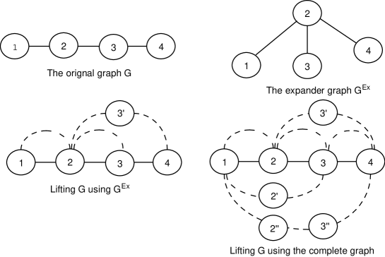
Figure 4: A caricature of lifting using expander. Let line graph $G$ be a line graph with $4$ nodes. We wish to use an expander $G^{Ex}$ with 4 nodes, shown on the top-right side of the figure. $G$ is lifted by adding paths that correspond to edges of expander. For example, an edge $(2,4)$ of expander is added as path $(2,3^{\prime},4)$. We also draw the lifting in [7] which uses the complete graph.

To this end, we consider the following multi-commodity flow: let $G^{Ex}=(V,E^{Ex})$ be an expander with a transition matrix $P^{Ex}$ and a stationary distribution $\pi$ as required – this is feasible since we have assumed $\pi_{max}=O(\pi_{0})$. We note that this assumption is used only for the existence of expanders. Consider a multi-commodity flow $f=(f^{st})_{(s,t)\in E^{Ex}}$ so that

• $val(f^{st})=\pi_{s}P^{Ex}_{st}=Q^{Ex}_{st},\forall(s,t)\in E^{Ex}$;

• $\sum_{s,t}f^{st}(ij)\leq KQ_{ij},\forall(i,j)\in E$;

Lemma 10.

There is a feasible multi-commodity flow in the above flow problem with congestion($K$) and path-length at most $W$, where $W=O^{*}(1/\Phi(P))$.

Proof..

The conclusion is derived directly from Claim 9 since the flow number $T$ is less than $12C=O^{*}(1/\Phi(P))$ and the flow considered is a balanced multi-commodity flow i.e. $W=24C=O^{*}(1/\Phi(P))$. $\Box$

Now, we can think of this multi-commodity flow as a weighted collection of directed paths $\{(\mathcal{P}_{r},w_{r}):1\leq r\leq N\}$, where the total weight of paths from node $s$ to $t$ is $\pi_{s}P^{Ex}_{st}$, where $(s,t)\in E^{Ex}$. Let $\ell_{r}$ be the length of path $\mathcal{P}_{r}$. From Lemma 10, we have the following:

$$\sum_{r}w_{r}=1,\ \ \ \ \ell_{r}\leq W,$$ (9)

$$\sum_{r:\mathcal{P}_{r}\text{ starts at }i}w_{r}=\pi_{i},\ \sum_{r:\mathcal{P}_{r}\text{ ends at }i}w_{r}=\pi_{i},~{}\mbox{for $i\in V$}$$ (10)

$$\sum_{r:(i,j)\in E(\mathcal{P}_{r})}w_{r}\leq WQ_{ij},~{}\mbox{for $(i,j)\in E$.}$$ (11)

Using such a collection of weighted paths, we construct the desired lifting next. As Figure 4, we construct the lifted graph $\widehat{G}=(\widehat{V},\widehat{E})$ from $G$ by adding a directed path $\mathcal{P}^{\prime}_{r}$ of length $\ell_{r}$ connecting $i$ to $j$ if $\mathcal{P}_{r}$ goes from $i$ to $j$. Subsequently, $\ell_{r}-1$ new nodes are added to the original graph. The ergodic flow on an edge $(i,j)$ of the lifted chain is defined by

$$\widehat{Q}_{ij}=\begin{cases}w_{r}/2W\ \ &\text{if}\ (i,j)\in E(\mathcal{P}^{\prime}_{r})\\ Q_{ij}-\sum_{r:ij\in E(\mathcal{P}_{r})}w_{r}/2W&\text{if}\ (i,j)\in E(G)\end{cases}$$

It is easy to check it defines a Markov chain on $\widehat{G}$, and a natural way of mapping the paths $\mathcal{P}^{\prime}_{r}$ onto the paths $\mathcal{P}_{r}$ collapses the random walk on $\widehat{G}$ onto the random walk on $G$. The stationary distribution of the lifted chain is

$$\widehat{\pi}_{i}=\begin{cases}w_{r}/2W\ \ &\text{if}\ i\in V({\mathcal{P}^{\prime}}_{r})\backslash V(G)\\ \pi_{i}-\sum_{r:\mathcal{P}_{r}\text{ thru }i}w_{r}/2W&\text{if}\ i\in V(G)\end{cases}$$

Thus, the above stated construction is a valid lifting of the given Markov chain $P$ defined on $G$.

6.3 Mixing time and size: Proof of Theorem 3

We prove two Lemmas about the performance of lifting we constructed, and they imply Theorem 3. At first, we state and prove the lemma which bounds the mixing time of the lifted chain we constructed.

Lemma 11.

The mixing time $\widehat{\mathcal{H}}$ of the lifted Markov chain represented by $\widehat{Q}$ defined on $\widehat{G}$ is $O^{*}(1/\Phi(P))$ .

Proof..

By the property of expanders, we have $\lambda_{P^{Ex}}=\Omega(1)$. Therefore, it is sufficient to show that

$$\widehat{\mathcal{H}}=O\left(\frac{W}{\lambda_{P^{Ex}}}\log\frac{1}{\pi_{0}}\right).$$

First, note that for any node $i\in V$ (i.e. a original node $i$ in $G$),

$$\frac{1}{2}\pi_{i}\leq\widehat{\pi}_{i}\leq\pi_{i}.$$ (12)

Now, under the lifted Markov chain the probability of getting on any directed path $\mathcal{P}^{\prime}_{r}$ starting at $i$ is

$$\widehat{P}_{ij}=\frac{\widehat{Q}_{ij}}{\widehat{\pi}_{i}}=\frac{w_{r}}{2W\widehat{\pi}_{i}}.$$

Hence the probability of getting on any directed path starting at $i$ is

$$\sum_{r:\mathcal{P}^{\prime}_{r}\text{ starts at }i}\frac{w_{r}}{2W\widehat{\pi}_{i}}=\frac{1}{2W\widehat{\pi}_{i}}\sum_{r:\mathcal{P}^{\prime}_{r}\text{ starts at }i}w_{r}=\frac{\pi_{i}}{2W\widehat{\pi}_{i}}.$$

From (12), this is bounded between $\frac{1}{2W},$ and $\frac{1}{W}$.

To study the $\widehat{\mathcal{H}}$, we will focus on the induced random walk (or Markov chain) on original nodes $V\subset\widehat{V}$ by the lifted Markov chain $\widehat{P}$. Let $\widehat{P}^{V}$ be the transition matrix of this induced random walk. Then,

$$\widehat{P}^{V}_{ij}=\widehat{P}_{ij}+\sum_{r:\mathcal{P}^{\prime}_{r}\text{ goes from }i\text{ to }j}\frac{w_{r}}{2W{\widehat{\pi}_{i}}}.$$

Now, $\widehat{P}^{V}\geq\widehat{P}\geq I/4$, because $\widehat{P}_{ii}=\widehat{Q}_{ii}/\widehat{\pi}_{i}\geq Q_{ii}/2\widehat{\pi}_{i}=P_{ii}\pi_{i}/2\widehat{\pi}_{i}\geq P_{ii}/2\geq I/4.$ Here we have assumed that $P\geq I/2$ as discussed earlier. Now,

$$\widehat{P}^{V}_{ij} \geq\frac{1}{2W{\widehat{\pi}_{i}}}\sum_{r:\mathcal{P}^{\prime}_{r}\text{ goes from }i\text{ to }j}w_{r}=\frac{\pi_{i}P^{Ex}_{ij}}{2W{\widehat{\pi}_{i}}}\geq\frac{1}{2W}P^{Ex}_{ij}.$$

And, its stationary distribution $\widehat{\pi}^{V}$ is : $\widehat{\pi}^{V}_{i}=\frac{\widehat{\pi}_{i}}{\widehat{\pi}(V)}.$ Therefore, by (12) we have $\frac{1}{2}\pi_{i}\leq\widehat{\pi}^{V}_{i}\leq 2\pi_{i}.$ Now, we can apply Claim 14 to obtain the following:

$$\lambda_{\widehat{P}^{V}(\widehat{P}^{V})^{*}}=\Omega\left(\frac{1}{W}\lambda_{P^{Ex}}\right).$$ (13)

Now, we are ready to design the following stopping rule $\Gamma$ that will imply that the desired bound on $\widehat{\mathcal{H}}$.

• Walk until visiting old nodes of $V\subset\widehat{V}$ for $T$ times, where $T:=\left\lceil 2\log(2/\widehat{\pi}^{V}_{0})/{\lambda_{\widehat{P}^{V}(\widehat{P}^{V})^{*}}}\right\rceil.$ Let this $T^{th}$ old node be denoted by $X$.

• Stop at $X$ with probability $1/2$.

• Otherwise, continue walking until getting onto any directed path $\mathcal{P}^{\prime}_{r}$; choose an interior node $Y$ of $\mathcal{P}^{\prime}_{r}$ uniformly at random and stop at $Y$.

From the relation (2) in Section 2.4 with $\varepsilon=\frac{1}{2}\sqrt{\widehat{\pi}^{V}_{0}}$, it follows that after time $T$ as defined above the Markov chain $\widehat{P}^{V}$, restricted to old nodes $V$, has distribution close to $\widehat{\pi}^{V}$ i.e.

$$|\Pr(X=w)-\widehat{\pi}^{V}_{w}|\leq\widehat{\pi}^{V}_{w}/2,~{}~{}\forall~{}w\in V.$$

According to the above stopping rule, we stop at an old node $w$ with probability $1/2$. Therefore, for any $w\in V$, we have that the stopping time $\Gamma$ stops at $w$ with probability at least $\widehat{\pi}^{V}_{w}/4\geq{\pi}_{w}/8\geq\widehat{\pi}_{w}/8$. With probability $1/2$, the rule does not stop at the node $X$. Let $w^{k}$ be the $k^{th}$ point in the walk starting from $X$. Because at any old node $i$, the probability of getting on any directed path is between $\frac{1}{2W}$ and $\frac{1}{W}$, a coupling argument shows that for any old node $i$,

$$\Pr(w^{k}=i|w^{0},\cdot,w^{k}\text{ are old nodes})\geq\left(1-\frac{1}{W}\right)^{k}\frac{1}{2}\widehat{\pi}^{V}_{i}$$

If $w$ is a new point on the directed path ${\mathcal{P}^{\prime}}_{r}$ which connects the old node $i$ to $j$. Then,

$$\Pr(\Gamma\text{~{}stop at }w) \geq\frac{1}{2}\sum_{k=0}^{\infty}\text{Prob}(w^{k}=i|w^{0},\cdot,w^{k}\text{ are old points})$$

$$~{}~{}~{}~{}~{}~{}~{}~{}~{}~{}~{}~{}~{}~{}~{}~{}\times\text{Prob}(\text{at }i\text{, get on the path~{}}{\mathcal{P}^{\prime}}_{r})\times\frac{1}{\ell_{r}}$$

$$\geq\frac{1}{2}\sum_{k=0}^{\infty}\left(1-\frac{1}{W}\right)^{k}\frac{1}{2}\widehat{\pi}^{V}_{i}\frac{w_{r}}{2W\widehat{\pi}_{i}}\frac{1}{W}$$

$$\geq\frac{w_{r}}{16W^{2}}\sum_{k=0}^{\infty}\left(1-\frac{1}{W}\right)^{k}$$

$$=\frac{w_{r}}{16W}$$

$$=\frac{1}{8}\widehat{\pi}_{w}$$

The average length of this stopping rule is $O(T+W)$. By (13),

$$O(T+W) =O\left(\left\lceil\frac{2}{\lambda_{\widehat{P}^{V}(\widehat{P}^{V})^{*}}}\log(2/\pi_{0})\right\rceil+W\right)=O\left(\frac{W}{\lambda_{P^{Ex}}}\log(1/\pi_{0})\right).$$

Thus, we have established that the stopping rule $\Gamma$ has the average length $O(W\log 1/\pi_{0})$ and the distribution of the stopping node is $\Omega(\widehat{\pi})$. Therefore, using the fill-up lemma stated in [1], it follows that $\widehat{\mathcal{H}}=O(W\log 1/\pi_{0})$. $\Box$

Also, we bound the size of the lifted chain we constructed as follows.

Lemma 12.

The size of the lifted Markov chain can be bounded above as $O^{*}(|E|/\Phi(P))$ .

Proof..

We want to establish that the size of the lifted chain in terms of the number of edges, i.e. $|\widehat{E}|=O^{*}(|E|/\Phi(P))$. Note that, the lifted graph $\widehat{G}$ is obtained by adding paths that appeared in the solution of the multi-commodity flow problem. Therefore, to establish the desired bound we need to establish a bound on the number of distinct paths as well as their lengths.

To this end, let us re-formulate the multi-commodity flow based on expander $G^{Ex}$ as follows. For each $(s,t)\in E^{Ex}$, we add a flow between $s$ and $t$. Let this flow be routed along possibly multiple paths. Let $P_{stj}$ denote the $j^{th}$ path from $s$ to $t$ and $x_{stj}$ be the amount of flow sent along this path. The length $\ell_{stj}$ of $P_{stj}$ is at most $W$ as the discussion in Lemma 10. Let the overall solution, denoted by $\{(\mathcal{P}_{r},w_{r})\}$, gives a feasible solution in the following polytope with $x_{stj}$ as its variables:

$$\sum_{j}x_{stj}=\pi_{s}P^{Ex}_{st},~{}~{}\forall(s,t)\in E^{Ex}$$

$$\sum_{st\in E^{Ex}}\sum_{j:e\in\mathcal{P}_{stj}}x_{stj}\leq WQ_{e},~{}~{}\forall e\in E$$

$$x_{stj}\geq 0\ \ \ \ \forall s,t,j.$$

Clearly, any feasible solution in this polytope, say $\{(\mathcal{P}_{r},w_{r})\}$, will work for our lifting construction. Now, the size of its support set is $|\{(\mathcal{P}_{r},w_{r})\}|$. If we consider the extreme point of this polytope, the size of its support set is at most $|E^{Ex}|+|E|=O(|E|)$ because the extreme point is an unique solution of a sub-collection of linear constraints in this polytope. Hence, if we choose such an extreme point $\{(\mathcal{P}_{r},w_{r})\}$ for our lifting, the size of our lifted chain $|\widehat{E}|$ is at most $O(W|E|)$ since each path is of length $O(W)$. Thus, we have established that the size of the lifted Markov chain is at most $O(W|E|)=O^{*}(|E|/\Phi(P))$. $\Box$

6.4 Useful Claims

We state and prove two useful claims which plays a key role in proving Lemma 11.

Claim 13.

Let $P_{1},P_{2}$ be reversible Markov chains with their stationary distributions $\pi_{1},\pi_{2}$ respectively. If there exist positive constants $\alpha,\beta,c,d$ such that $P_{1}\geq\alpha P_{2}$, $P_{1}\geq\beta I$ and $c\pi_{2}\leq\pi_{1}\leq d\pi_{2}$, then

$$\lambda_{P_{1}}\geq\min\left(\frac{\alpha c}{d^{2}}\lambda_{P_{2}},2\beta\right).$$

Proof..

From the min-max characterization of the spectral gap (see, e.g., the page 176 in [14]) for the reversible Markov chain, it follows that

$$\lambda_{P_{1}} =~{}\inf_{\psi:V\rightarrow\mathbb{R}}\left(\frac{\sum_{i,j\in V}(\psi(i)-\psi(j))^{2}(\pi_{1})_{i}(P_{1})_{ij}}{\sum_{i,j\in V}(\psi(i)-\psi(j))^{2}(\pi_{1})_{i}(\pi_{1})_{j}}\right)$$

$$\geq\left(\frac{\alpha c}{d^{2}}\right)\inf_{\psi:V\rightarrow\mathbb{R}}\left(\frac{\sum_{i,j\in V}(\psi(i)-\psi(j))^{2}(\pi_{2})_{i}(P_{2})_{ij}}{\sum_{i,j\in V}(\psi(i)-\psi(j))^{2}(\pi_{2})_{i}(\pi_{2})_{j}}\right)$$

$$=\left(\frac{\alpha c}{d^{2}}\right)\lambda_{P_{2}}.$$

The smallest eigenvalue of $P_{1}$ is greater than $2\beta-1$ because $P_{1}\geq\beta I$. So, the distance between the smallest eigenvalue and -1 is greater than $2\beta$. This completes the proof. $\Box$

Claim 14.

Let $P_{1},P_{2}$ be Markov chains with their stationary distributions $\pi_{1},\pi_{2}$ respectively. Now, suppose $P_{2}$ is reversible. ($P_{1}$ is not necessarily reversible.) If there exist positive constants $\alpha,\beta,c,d$ such that $P_{1}\geq\alpha P_{2}$, $P_{1}\geq\beta I$ and $c\pi_{2}\leq\pi_{1}\leq d\pi_{2}$, then

$$\lambda_{P_{1}P^{*}_{1}}\geq\min\left(\frac{\alpha\beta c}{d^{2}}\lambda_{P_{2}},2\beta^{2}\right).$$

Proof..

$P_{1}P^{*}_{1}$ is a reversible Markov chain which has $\pi_{1}$ as its stationary distribution. Because $P^{*}_{1}\geq\beta I$, $P_{1}P^{*}_{1}\geq\alpha P_{2}P^{*}_{1}\geq\alpha\beta P_{2}.$ Also, $P_{1}P^{*}_{1}\geq\beta^{2}I$. Now, the proof follows from Claim 13. $\Box$

7 Conclusion

Motivated by applications arising in emerging networks such as sensor networks, peer-to-peer networks and surveillance network of unmanned vehicles, we consider the question of designing fast linear iterative algorithms for computing the average of numbers in a network. We presented a novel construction of such an algorithm by designing the fastest mixing non-reversible Markov chain on any given graph. Our Markov chain obtained through a new notion denoted by pseudo-lifting. We apply our constructions to graphs with geometry, or graphs with doubling dimension. By using their topological properties explicitly, we obtain fast and slim pseudo-lifted Markov chains. The effectiveness (and optimality) of our constructions are explained through various examples. As a byproduct, our result provides the fastest mixing Markov chain for any given graph which should be of interest in its own right. Our result should naturally find their applications in the context of distributed optimization, estimation and control.

We note that the pseudo-lifting presented here is based on a two-level “hierarchical star” topology. This construction is less robust to node failures. For example, failure of “root” node can increase the mixing time drastically. To address this, one may alternatively use a “hierarchical expander” based pseudo-lifting. That is, in place of the “star” topology in the pseudo-lifting, utilize the “expader” topology. This will naturally make the construction more robust without loss of performance. Of course, this will complicate the mixing time analysis drastically. This is where our method developed in the expander-based lifting will be readily useful.

References

- [1] D. J. Aldous. Some inequalities for reversible Markov chains. In J. London Math. Soc. 25, pages 564–576, 1982.
- [2] P. Assouad. Plongements lipschitziens dans . Bull. Soc. Math. France, 111(4):429–448, 1983.
- [3] V. D. Blondel, J. M. Hendrickx, A. Olshevsky, and J. N. Tsitsiklis. Convergence in multiagent coordination, consensus, and flocking. In Joint 44th IEEE Conference on Decision and Control and European Control Conference (CDC-ECC’05).
- [4] S. Boyd, P. Diaconis, and L. Xiao. Fastest mixing Markov chain on a graph. SIAM Review, 46(4):667–689, 2004.
- [5] Stephen Boyd, Arpita Ghosh, Balaji Prabhakar, and Devavrat Shah. Gossip algorithms: Design, analysis and applications. In Proceedings of IEEE INFOCOM 2005, pages 1653–1664, 2005.
- [6] Stephen Boyd, Arpita Ghosh, Balaji Prabhakar, and Devavrat Shah. Randomized gossip algorithms. IEEE/ACM Trans. Netw., 14(SI):2508–2530, 2006.
- [7] F. Chen, L. Lovász, and I. Pak. Lifting Markov chains to speed up mixing. In STOC ’99: Proceedings of the thirty-sixth annual ACM symposium on Theory of computing, pages 275–281, New York, NY, USA, 1999. ACM Press.
- [8] Sanjoy Dasgupta and Yoav Freund. Random projection trees and low dimensional manifolds. In STOC ’08: Proceedings of the 40th annual ACM symposium on Theory of computing, pages 537–546, New York, NY, USA, 2008. ACM.
- [9] P. Diaconis, S. Holmes, and R. Neal. Analysis of a non-reversible Markov chain sampler. Ann. Appl. Probab., 10:726–752, 2000.
- [10] A. G. Dimakis, A.D. Sarwate, and M.J. Wainwright. Geographic gossip : Efficient aggregation for sensor networks. In 5th International ACM/IEEE Symposium on Information Processing in Sensor Networks (IPSN ’06), April 2006.
- [11] Anupam Gupta, Robert Krauthgamer, and James R. Lee. Bounded geometries, fractals, and low-distortion embeddings. In FOCS ’03: Proceedings of the 44th Annual IEEE Symposium on Foundations of Computer Science, page 534, Washington, DC, USA, 2003. IEEE Computer Society.
- [12] W.K. Hastings. Monte Carlo sampling methods using Markov chains and their applications. Biometrika, 57:97–109, 1970.
- [13] Juha Heinonen, editor. Lectures on Analysis on Metric Spaces. Springer, 2001.
- [14] R. Horn and C. Johnson, editors. Matrix Analysis. Cambridge Univ. Press., 1985.
- [15] A. Jadbabaie, J. Lin, and A. Morse. Coordination of groups of mobile autonomous agents using nearest neighbor rules. IEEE Trans. Autom. Control, 48(6):988–1001, 2003.
- [16] David Kempe, Alin Dobra, and Johannes Gehrke. Gossip-based computation of aggregate information. In FOCS ’03: Proceedings of the 44th Annual IEEE Symposium on Foundations of Computer Science, page 482, Washington, DC, USA, 2003. IEEE Computer Society.
- [17] David Kempe and Frank McSherry. A decentralized algorithm for spectral analysis. In STOC ’04: Proceedings of the thirty-sixth annual ACM symposium on Theory of computing, pages 561–568, New York, NY, USA, 2004. ACM Press.
- [18] Claire Kenyon, Elchanan Mossel, and Yuval Peres. Glauber dynamics on trees and hyperbolic graphs. In IEEE Symposium on Foundations of Computer Science, pages 568–578, 2001.
- [19] P. Kolman and C. Scheideler. Improved bounds for the unsplittable flow problem. In SODA ’02: Proceedings of the 13th annual ACM-SIAM symposium on Discrete algorithms, pages 184–193, Philadelphia, PA, USA, 2002. Society for Industrial and Applied Mathematics.
- [20] Manolis Koubarakis, Christos Tryfonopoulos, Stratos Idreos, and Yannis Drougas. Selective information dissemination in p2p networks: problems and solutions. SIGMOD Rec., 32(3):71–76, 2003.
- [21] Tom Leighton and Satish Rao. Multicommodity max-flow min-cut theorems and their use in designing approximation algorithms. In FOCS ’88: Proceedings of the 29th Annual Symposium on Foundations of Computer Science, pages 422–431, 1988.
- [22] Laszlo Lovasz and Peter Winkler. Mixing times. Microsurveys in Discrete Probability (ed. D. Aldous and J. Propp), DIMACS Series in Discrete Math. and theor. Comp. Sci., pages 85–133, 1998.
- [23] Samuel Madden, Michael J. Franklin, Joseph M. Hellerstein, and Wei Hong. Tag: a tiny aggregation service for ad-hoc sensor networks. SIGOPS Oper. Syst. Rev., 36(SI):131–146, 2002.
- [24] Dmitry M. Malioutov, Jason K. Johnson, and Alan S. Willsky. Walk-sums and belief propagation in gaussian graphical models. J. Mach. Learn. Res., 7:2031–2064, 2006.
- [25] N. Metropolis, A.W. Rosenbluth, M.N. Rosenbluth, A.H. Teller, and E. Teller. Equations of state calculations by fast computing machines. Journal of Chemical Physics, 21:1087–1092, 1953.
- [26] D. Mosk-Aoyama and D. Shah. Fast distributed algorithms for computing separable functions. IEEE Transaction on Information Theory, 54(7):2997–3007, 2008.
- [27] A. Nedic and A. Ozdaglar. Distributed subgradient methods for multi-agent optimization. LIDS report 2755, to appear in IEEE Transactions on Automatic Control, 2008.
- [28] P.Diaconis and L.Saloff-Coste. Moderate growth and random walk on finite groups. Geometric and Functional Analysis, 4(1), 1994.
- [29] J. Sun S. Boyd, P. Diaconis and L. Xiao. Fastest mixing Markov chain on a path. In The American Mathematical Monthly, pages 113(1):70–74, 2006.
- [30] K. Savla, F. Bullo, and E. Frazzoli. On traveling salesperson problems for Dubins’ vehicle: stochastic and dynamic environments. pages 4530–4535, Seville, Spain, December 2005.
- [31] J. Tsitsiklis. Problems in decentralized decision making and computation. Ph.D. dissertation, Lab. Information and Decision Systems, MIT, Cambridge, MA, 1984.
- [32] L. Xiao and S. Boyd. Fast linear iterations for distributed averaging. In Systems and Control Letters, pages 53:65–78, 2004.