Prodsimplicial-Neighborly Polytopes

Abstract.

Simultaneously generalizing both neighborly and neighborly cubical polytopes, we introduce PSN polytopes: their $k$-skeleton is combinatorially equivalent to that of a product of $r$ simplices.

We construct PSN polytopes by three different methods, the most versatile of which is an extension of Sanyal & Ziegler’s “projecting deformed products” construction to products of arbitrary simple polytopes. For general $r$ and $k$, the lowest dimension we achieve is $2k+r+1$.

Using topological obstructions similar to those introduced by Sanyal to bound the number of vertices of Minkowski sums, we show that this dimension is minimal if we additionally require that the PSN polytope is obtained as a projection of a polytope that is combinatorially equivalent to the product of $r$ simplices, when the dimensions of these simplices are all large compared to $k$.

1. Introduction

1.1. Definitions

Let $\triangle_{n}$ denote the $n$-dimensional simplex. For any tuple $\underline{n}\mbox{~{}\raisebox{0.86108pt}{\scriptsize$\mathrm{:}$}$=$ }(n_{1},\dots,n_{r})$ of integers, we denote by $\triangle_{\underline{n}}$ the product of simplices $\triangle_{n_{1}}\times\dots\times\triangle_{n_{r}}$. This is a polytope of dimension $\sum n_{i}$, whose non-empty faces are obtained as products of non-empty faces of the simplices $\triangle_{n_{1}},\dots,\triangle_{n_{r}}$. For example, Figure 1 represents the graphs of $\triangle_{i}\times\triangle_{6}$, for ${i\in\{1,2,3\}}$.

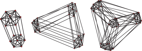
Figure 1. The graphs of the products $\triangle_{(i,6)}=\triangle_{i}\times\triangle_{6}$, for $i\in\{1,2,3\}$.

We are interested in polytopes with the same “initial” structure as these products.

Definition 1.1.

Let $k\geq 0$ and $\underline{n}\mbox{~{}\raisebox{0.86108pt}{\scriptsize$\mathrm{:}$}$=$ }(n_{1},\dots,n_{r})$, with $r\geq 1$ and $n_{i}\geq 1$ for all $i$. A convex polytope in some Euclidean space is $(k,\underline{n})$-prodsimplicial-neighborly — or $(k,\underline{n})$-PSN for short — if its $k$-skeleton is combinatorially equivalent to that of $\triangle_{\underline{n}}\mbox{~{}\raisebox{0.86108pt}{\scriptsize$\mathrm{:}$}$=$ }\triangle_{n_{1}}\times\dots\times\triangle_{n_{r}}$.

We choose the term “prodsimplicial” to shorten “product simplicial”. This definition is essentially motivated by two particular classes of PSN polytopes:

1. neighborly polytopes arise when $r=1$;

2. neighborly cubical polytopes [JS07, SZ09] arise when $\underline{n}=(1,1,\dots,1)$.

Remark 1.2.

In the literature, a polytope is $k$-neighborly if any subset of at most $k$ of its vertices forms a face. Observe that such a polytope is $(k-1,n)$-PSN with our notation.

The product $\triangle_{\underline{n}}$ is a $(k,\underline{n})$-PSN polytope of dimension $\sum n_{i}$, for each $k$ with ${0\leq k\leq\sum n_{i}}$. We are naturally interested in finding $(k,\underline{n})$-PSN polytopes of smaller dimensions. For example, the cyclic polytope $C_{2k+2}(n+1)$ is a $(k,n)$-PSN polytope of dimension $2k+2$. We denote by $\delta(k,\underline{n})$ the smallest possible dimension of a $(k,\underline{n})$-PSN polytope.

PSN polytopes can be obtained by projecting the product $\triangle_{\underline{n}}$, or a combinatorially equivalent polytope, onto a smaller subspace. For example, the cyclic polytope $C_{2k+2}(n+1)$ (just like any polytope with $n+1$ vertices) can be seen as a projection of the simplex $\triangle_{n}$ to $\mathbb{R}^{2k+2}$.

Definition 1.3.

A $(k,\underline{n})$-PSN polytope is $(k,\underline{n})$-projected-prodsimplicial-neighborly — or $(k,\underline{n})$-PPSN for short — if it is a projection of a polytope that is combinatorially equivalent to $\triangle_{\underline{n}}$.

We denote by $\delta_{pr}(k,\underline{n})$ the smallest possible dimension of a $(k,\underline{n})$-PPSN polytope.

1.2. Outline and main results

The present paper may be naturally divided into two parts. In the first part, we present three methods for constructing low-dimensional PPSN polytopes:

1. Reflections of cyclic polytopes;

2. Minkowski sums of cyclic polytopes;

3. Deformed Product constructions in the spirit of Sanyal & Ziegler [Zie04, SZ09].

The second part derives topological obstructions for the existence of such objects, using techniques developed by Sanyal in [San09] (see also [RS09]) to bound the number of vertices of Minkowski sums. In view of these obstructions, our constructions in the first part turn out to be optimal for a wide range of parameters.

We devote the remainder of the introduction to highlighting our most relevant results. To facilitate the navigation in the article, we label each result by the number it actually receives later on.

Constructions.

Our first non-trivial example is a $(k,(1,n))$-PSN polytope in dimension ${2k+2}$, obtained by reflecting the cyclic polytope $C_{2k+2}(n+1)$ through a well-chosen hyperplane:

Proposition 2.3. For any $k\geq 0$, $n\geq 2k+2$ and $\lambda\in\mathbb{R}$ sufficiently large, the polytope

$$P\ \mbox{~{}\raisebox{0.86108pt}{\scriptsize$\mathrm{:}$}$=$ }\ \mathrm{conv}\left(\big{\{}(t_{i},\dots,t_{i}^{2k+2})^{T}\ |\ i\in[n+1]\big{\}}\ \cup\ \big{\{}(t_{i},\dots,t_{i}^{2k+1},\lambda-t_{i}^{2k+2})^{T}\ |\ i\in[n+1]\big{\}}\right)$$

is a $(k,(1,n))$-PSN polytope of dimension $2k+2$.

For example, this provides us with a $4$-dimensional polytope whose graph is the cartesian product $K_{2}\times K_{n}$, for any $n\geq 3$.

Next, forming a well-chosen Minkowski sum of cyclic polytopes yields explicit coordinates for $(k,\underline{n})$-PPSN polytopes:

Theorem 2.6. Let $k\geq 0$ and $\underline{n}\mbox{~{}\raisebox{0.86108pt}{\scriptsize$\mathrm{:}$}$=$ }(n_{1},\dots,n_{r})$ with $r\geq 1$ and $n_{i}\geq 1$ for all $i$. There exist index sets $I_{1},\dots,I_{r}\subset\mathbb{R}$, with $|I_{i}|=n_{i}$ for all $i$, such that the polytope

$$P\ \mbox{~{}\raisebox{0.86108pt}{\scriptsize$\mathrm{:}$}$=$ }\ \mathrm{conv}\{w_{a_{1},\dots,a_{r}}\ |\ (a_{1},\dots,a_{r})\in I_{1}\times\dots\times I_{r}\}\ \subset\ \mathbb{R}^{2k+r+1}$$

is $(k,\underline{n})$-PPSN, where $w_{a_{1},\dots,a_{r}}\mbox{~{}\raisebox{0.86108pt}{\scriptsize$\mathrm{:}$}$=$ }\big{(}a_{1},\dots,a_{r},\sum_{i\in[r]}a_{i}^{2},\dots,\sum_{i\in[r]}a_{i}^{2k+2}\big{)}^{T}.$ Consequently,

$$\delta(k,\underline{n})\ \leq\ \delta_{pr}(k,\underline{n})\ \leq\ 2k+r+1.$$

For $r=1$ we recover neighborly polytopes.

Finally, we extend Sanyal & Ziegler’s technique of “projecting deformed products of polygons” [Zie04, SZ09] to products of arbitrary simple polytopes: given a polytope $P$ that is combinatorially equivalent to a product of simple polytopes, we exhibit a suitable projection that preserves the complete $k$-skeleton of $P$. More concretely, we describe how to use colorings of the graphs of the polar polytopes of the factors in the product to raise the dimension of the preserved skeleton. The basic version of this technique yields the following result:

Proposition 3.4. Let $P_{1},\dots,P_{r}$ be simple polytopes of respective dimension $n_{i}$, and with $m_{i}$ many facets. Let $\chi_{i}\mbox{~{}\raisebox{0.86108pt}{\scriptsize$\mathrm{:}$}$=$ }\chi(\text{sk}_{1}P_{i}^{\triangle})$ denote the chromatic number of the graph of the polar polytope $P_{i}^{\triangle}$. For a fixed integer $d\leq\sum_{i=1}^{r}n_{i}$, let $t$ be maximal such that $\sum_{i=1}^{t}n_{i}\leq d$. Then there exists a $d$-dimensional polytope whose $k$-skeleton is combinatorially equivalent to that of the product $P_{1}\times\dots\times P_{r}$ provided

$$0\ \leq\ k\ \leq\ \sum_{i=1}^{r}(n_{i}-m_{i})+\sum_{i=1}^{t}(m_{i}-\chi_{i})+\left\lfloor\frac{1}{2}\left(d-1+\sum_{i=1}^{t}(\chi_{i}-n_{i})\right)\right\rfloor.$$

A family of polytopes that minimize the last summand are products of even polytopes (all 2-dimensional faces have an even number of vertices). See Example 3.5 for the details, and the end of Section 3.1 for extensions of this technique.

Specializing the factors to simplices provides another construction of PPSN polytopes. When some of these simplices are small compared to $k$, this technique in fact yields our best examples of PPSN polytopes:

Theorem 3.8. For any $k\geq 0$ and $\underline{n}\mbox{~{}\raisebox{0.86108pt}{\scriptsize$\mathrm{:}$}$=$ }(n_{1},\dots,n_{r})$ with ${1=n_{1}=\dots=n_{s}<n_{s+1}\leq\dots\leq n_{r}}$,

$$\delta_{pr}(k,\underline{n})\ \leq\ \begin{cases}2(k+r)-s-t&\text{if }3s\leq 2k+2r,\\ 2(k+r-s)+1&\text{if }3s=2k+2r+1,\\ 2(k+r-s+1)&\text{if }3s\geq 2k+2r+2,\end{cases}$$

where $t\in\{s,\dots,r\}$ is maximal such that $3s+\sum_{i=s+1}^{t}(n_{i}+1)\ \leq\ 2k+2r$.

If $n_{i}=1$ for all $i$, we recover the neighborly cubical polytopes of [SZ09].

Obstructions

In order to derive lower bounds on the minimal dimension $\delta_{pr}(k,\underline{n})$ that a $(k,\underline{n})$-PPSN polytope can have, we apply and extend a method due to Sanyal [San09]. For any projection which preserves the $k$-skeleton of $\triangle_{\underline{n}}$, we use Gale duality to construct a simplicial complex that can be embedded in a certain dimension. The argument is then a topological obstruction based on Sarkaria’s criterion for the embeddability of a simplicial complex in terms of colorings of Kneser graphs [Mat03]. We obtain the following result:

Corollary 4.13. Let $\underline{n}\mbox{~{}\raisebox{0.86108pt}{\scriptsize$\mathrm{:}$}$=$ }(n_{1},\dots,n_{r})$ with $1=n_{1}=\dots=n_{s}<n_{s+1}\leq\dots\leq n_{r}$.

1. If

   $$0\ \leq\ k\ \leq\ \sum_{i=s+1}^{r}\left\lfloor\frac{n_{i}-2}{2}\right\rfloor+\max\left\{0,\left\lfloor\frac{s-1}{2}\right\rfloor\right\},$$

   then $\delta_{pr}(k,\underline{n})\geq 2k+r-s+1$.

2. If $k\geq\left\lfloor\frac{1}{2}\sum_{i}n_{i}\right\rfloor$ then $\delta_{pr}(k,\underline{n})\geq\sum_{i}n_{i}$.

In particular, the upper and lower bounds provided by Theorem 2.6 and Corollary 4.13 match over a wide range of parameters:

Theorem 1.4.

Let $\underline{n}\mbox{~{}\raisebox{0.86108pt}{\scriptsize$\mathrm{:}$}$=$ }(n_{1},\dots,n_{r})$ with $r\geq 1$ and $n_{i}\geq 2$ for all $i$. For any $k$ such that $0\leq k\leq\sum_{i\in[r]}\left\lfloor\frac{n_{i}-2}{2}\right\rfloor$, the smallest $(k,\underline{n})$-PPSN polytope has dimension exactly $2k+r+1$. In other words:

$$\delta_{pr}(k,\underline{n})\ =\ 2k+r+1.$$

Remark 1.5.

During the final stages of completing this paper, we learned that Rörig and Sanyal [RS09] also applied Sanyal’s topological obstruction method to derive lower bounds on the target dimension of a projection preserving skeleta of different kind of products (products of polygons, products of simplices, and wedge products of polytopes). In particular, for a product $\triangle_{n}\times\dots\times\triangle_{n}$ of $r$ identical simplices, $r\geq 2$, they obtain our Theorem 4.9 and a result (their Theorem 4.5) that is only slightly weaker than Theorem 4.12 in this setting (compare with Sections 4.5 and 4.6).

2. Constructions from cyclic polytopes

Let $t\mapsto\mu_{d}(t)\mbox{~{}\raisebox{0.86108pt}{\scriptsize$\mathrm{:}$}$=$ }(t,t^{2},\dots,t^{d})^{T}$ be the moment curve in $\mathbb{R}^{d}$, $t_{1}<t_{2}<\dots<t_{n}$ be $n$ distinct real numbers and $C_{d}(n)\mbox{~{}\raisebox{0.86108pt}{\scriptsize$\mathrm{:}$}$=$ }\mathrm{conv}\{\mu_{d}(t_{i})\ |\ i\in[n]\}$ denote the cyclic polytope in its realization on the moment curve. We refer to [Zie95, Theorem 0.7] and [dLRS10, Corollary 6.1.9] for combinatorial properties of $C_{d}(n)$, in particular Gale’s Evenness Criterion which characterizes the index sets of upper and lower facets of $C_{d}(n)$.

Cyclic polytopes yield our first examples of PSN polytopes:

Example 2.1.

For any integers $k\geq 0$ and $n\geq 2k+2$, the cyclic polytope ${C_{2k+2}(n+1)}$ is $(k,n)$-PPSN.

Example 2.2.

For any $k\geq 0$ and $\underline{n}\mbox{~{}\raisebox{0.86108pt}{\scriptsize$\mathrm{:}$}$=$ }(n_{1},\dots,n_{r})$ with $r\geq 1$ and $n_{i}\geq 1$ for all $i$, define $I\mbox{~{}\raisebox{0.86108pt}{\scriptsize$\mathrm{:}$}$=$ }\{i\in[r]\ |\ n_{i}\geq 2k+3\}$. Then the product

$$\prod_{i\in I}C_{2k+2}(n_{i}+1)\times\prod_{i\notin I}\triangle_{n_{i}}$$

is a $(k,\underline{n})$-PPSN polytope of dimension $(2k+2)|I|+\sum_{i\notin I}n_{i}$ (which is smaller than $\sum n_{i}$ when $I$ is nonempty). Consequently,

$$\delta(k,\underline{n})\ \leq\ \delta_{pr}(k,\underline{n})\ \leq\ (2k+2)|I|+\sum_{i\notin I}n_{i}.$$

2.1. Reflections of cyclic polytopes

Our next example deals with the special case of the product $\triangle_{1}\times\triangle_{n}$ of a segment with a simplex. Using products of cyclic polytopes as in Example 2.2, we can realize the $k$-skeleton of this polytope in dimension $2k+3$. We can lower this dimension by $1$ by reflecting the cyclic polytope $C_{2k+2}(n+1)$ through a well-chosen hyperplane:

Proposition 2.3.

For any $k\geq 0$, $n\geq 2k+2$ and $\lambda\in\mathbb{R}$ sufficiently large, the polytope

$$P\ \mbox{~{}\raisebox{0.86108pt}{\scriptsize$\mathrm{:}$}$=$ }\ \mathrm{conv}\left(\big{\{}(t_{i},\dots,t_{i}^{2k+2})^{T}\ |\ i\in[n+1]\big{\}}\ \cup\ \big{\{}(t_{i},\dots,t_{i}^{2k+1},\lambda-t_{i}^{2k+2})^{T}\ |\ i\in[n+1]\big{\}}\right)$$

is a $(k,(1,n))$-PSN polytope of dimension $2k+2$.

Proof.

The polytope $P$ is obtained as the convex hull of two copies of the cyclic polytope $C_{2k+2}(n+1)$. The first one $Q\mbox{~{}\raisebox{0.86108pt}{\scriptsize$\mathrm{:}$}$=$ }\mathrm{conv}\{\mu_{2k+2}(t_{i})\ |\ i\in[n+1]\}$ lies on the moment curve $\mu_{2k+2}$, while the second one is obtained as a reflection of $Q$ with respect to a hyperplane that is orthogonal to the last coordinate vector $u_{2k+2}$ and sufficiently far away. During this process,

1. we destroy all the faces of $Q$ only contained in upper facets of $Q$;

2. we create prisms over faces of $Q$ that lie in at least one upper and one lower facet of $Q$. In other words, we create prisms over the faces of $Q$ strictly preserved under the orthogonal projection $\pi:\mathbb{R}^{2k+2}\to\mathbb{R}^{2k+1}$ with kernel $\mathbb{R}u_{2k+2}$.

The projected polytope $\pi(Q)$ is nothing but the cyclic polytope $C_{2k+1}(n+1)$. Since this polytope is $k$-neighborly, any face $F$ of dimension at most $k-1$ in $Q$ is strictly preserved by $\pi$. Thus, we take the prism over all faces of $Q$ of dimension at most $k-1$.

Thus, in order to complete the proof that the $k$-skeleton of $P$ is that of $\triangle_{1}\times\triangle_{n}$, it is enough to show that any $k$-face of $Q$ remains in $P$. This is obviously the case if this $k$-face is also a $k$-face of $C_{2k+1}(n+1)$, and follows from the next combinatorial lemma otherwise. ∎

Lemma 2.4.

A $k$-face of $C_{2k+2}(n+1)$ which is not a $k$-face of $C_{2k+1}(n+1)$ is only contained in lower facets of $C_{2k+2}(n+1)$.

Proof.

Let $F\subset[n+1]$ be a $k$-face of $C_{2k+2}(n+1)$. We assume that $F$ is contained in at least one upper facet $G\subset[n+1]$ of $C_{2k+2}(n+1)$. Since the size of the final block of an upper facet of a cyclic polytope is odd, $G$ contains $n+1$. If $n+1\in G\smallsetminus F$, then $G\smallsetminus\{n+1\}$ is a facet of $C_{2k+1}(n+1)$ containing $F$. Otherwise, $n+1\in F$, and $F^{\prime}\mbox{~{}\raisebox{0.86108pt}{\scriptsize$\mathrm{:}$}$=$ }F\smallsetminus\{n+1\}$ has only $k$ elements. Thus, $F^{\prime}$ is a face of $C_{2k}(n)$, and can be completed to a facet of $C_{2k}(n)$. Adding the index $n+1$ back to this facet, we obtain a facet of $C_{2k+1}(n+1)$ containing $F$. In both cases, we have shown that $F$ is a $k$-face of $C_{2k+1}(n+1)$. ∎

2.2. Minkowski sums of cyclic polytopes

Our next examples are Minkowski sums of cyclic polytopes. We first describe an easy construction that avoids all technicalities, but only yields $(k,\underline{n})$-PPSN polytopes in dimension $2k+2r$. After that, we show how to reduce the dimension to $2k+r+1$, which according to Corollary 4.13 is best possible for large $n_{i}$’s.

Proposition 2.5.

Let $k\geq 0$ and $\underline{n}\mbox{~{}\raisebox{0.86108pt}{\scriptsize$\mathrm{:}$}$=$ }(n_{1},\dots,n_{r})$ with $r\geq 1$ and $n_{i}\geq 1$ for all $i$. For any pairwise disjoint index sets $I_{1},\dots,I_{r}\subset\mathbb{R}$, with $|I_{i}|=n_{i}$ for all $i$, the polytope

$$P\ \mbox{~{}\raisebox{0.86108pt}{\scriptsize$\mathrm{:}$}$=$ }\ \mathrm{conv}\big{\{}v_{a_{1},\dots,a_{r}}\ |\ (a_{1},\dots,a_{r})\in I_{1}\times\dots\times I_{r}\big{\}}\ \subset\ \mathbb{R}^{2k+2r}$$

is $(k,\underline{n})$-PPSN, where

$$v_{a_{1},\dots,a_{r}}\ \mbox{~{}\raisebox{0.86108pt}{\scriptsize$\mathrm{:}$}$=$ }\ \left(\sum_{i\in[r]}a_{i},\sum_{i\in[r]}a_{i}^{2},\dots,\sum_{i\in[r]}a_{i}^{2k+2r}\right)^{T}\in\mathbb{R}^{2k+2r}.$$

Proof.

The vertex set of $\triangle_{\underline{n}}$ is indexed by $I_{1}\times\dots\times I_{r}$. Let $A\mbox{~{}\raisebox{0.86108pt}{\scriptsize$\mathrm{:}$}$=$ }A_{1}\times\dots\times A_{r}\subset I_{1}\times\dots\times I_{r}$ define a $k$-face of $\triangle_{\underline{n}}$. Consider the polynomial

$$f(t)\ \mbox{~{}\raisebox{0.86108pt}{\scriptsize$\mathrm{:}$}$=$ }\ \prod_{i\in[r]}\prod_{a\in A_{i}}(t-a)^{2}\ =\ \sum_{j=0}^{2k+2r}c_{j}t^{j}.$$

Since $A$ indexes a $k$-face of $\triangle_{\underline{n}}$, we know that $\sum|A_{i}|=k+r$, so that the degree of $f(t)$ is indeed $2k+2r$. Since $f(t)\geq 0$, and equality holds if and only if $t\in\bigcup_{i\in[r]}A_{i}$, the inner product $(c_{1},\dots,c_{2k+2r})\cdot v_{a_{1},\dots,a_{r}}$ equals

$$(c_{1},\dots,c_{2k+2r})\begin{pmatrix}\sum_{i\in[r]}a_{i}\\ \vdots\\ \sum_{i\in[r]}a_{i}^{2k+2r}\end{pmatrix}\ =\ \sum_{i\in[r]}\sum_{j=1}^{2k+2r}c_{j}a_{i}^{j}\ =\ \sum_{i\in[r]}\big{(}f(a_{i})-c_{0}\big{)}\ \geq\ -rc_{0},$$

with equality if and only if $(a_{1},\dots,a_{r})\in A$. Thus, $A$ indexes a face of $P$ defined by the linear inequality $\sum_{i\in[r]}c_{i}x_{i}\geq-rc_{0}$.

We thus obtain that the $k$-skeleton of $P$ completely contains the $k$-skeleton of $\triangle_{\underline{n}}$. Since $P$ is furthermore a projection of $\triangle_{\underline{n}}$, the faces of $\triangle_{\underline{n}}$ are the only candidates to be faces of $P$. We conclude that the $k$-skeleton of $P$ is actually combinatorially equivalent to that of $\triangle_{\underline{n}}$. ∎

To realize the $k$-skeleton of $\triangle_{n_{1}}\times\dots\times\triangle_{n_{r}}$ even in dimension $2k+r+1$, we slightly modify this construction in the following way.

Theorem 2.6.

Let $k\geq 0$ and $\underline{n}\mbox{~{}\raisebox{0.86108pt}{\scriptsize$\mathrm{:}$}$=$ }(n_{1},\dots,n_{r})$ with $r\geq 1$ and $n_{i}\geq 1$ for all $i$. There exist pairwise disjoint index sets $I_{1},\dots,I_{r}\subset\mathbb{R}$, with $|I_{i}|=n_{i}$ for all $i$, such that the polytope

$$P\ \mbox{~{}\raisebox{0.86108pt}{\scriptsize$\mathrm{:}$}$=$ }\ \mathrm{conv}\{w_{a_{1},\dots,a_{r}}\ |\ (a_{1},\dots,a_{r})\in I_{1}\times\dots\times I_{r}\}\ \subset\ \mathbb{R}^{2k+r+1}$$

is $(k,\underline{n})$-PPSN, where

$$w_{a_{1},\dots,a_{r}}\ \mbox{~{}\raisebox{0.86108pt}{\scriptsize$\mathrm{:}$}$=$ }\ \bigg{(}a_{1},\dots,a_{r},\sum_{i\in[r]}a_{i}^{2},\dots,\sum_{i\in[r]}a_{i}^{2k+2}\bigg{)}^{T}\in\mathbb{R}^{2k+r+1}.$$

Proof.

We will choose the index sets $I_{1},\dots,I_{r}$ to be sufficiently separated in a sense that will be made explicit later in the proof. For each $k$-face $F$ of $\triangle_{\underline{n}}$, indexed by $A_{1}\times\dots\times A_{r}\subset I_{1}\times\dots\times I_{r}$, our choice of the $I_{i}$’s will ensure the existence of a monic polynomial

$$f_{F}(t)\ \mbox{~{}\raisebox{0.86108pt}{\scriptsize$\mathrm{:}$}$=$ }\ \sum_{j=0}^{2k+2}c_{j}t^{j},$$

which, for all $i\in[r]$, can be decomposed as

$$f_{F}(t)\ =\ Q_{i}(t)\prod_{a\in A_{i}}(t-a)^{2}+s_{i}t+r_{i},$$

where $Q_{i}(t)$ is an everywhere positive polynomial of degree $2k+2-2|A_{i}|$, and $r_{i},s_{i}\in\mathbb{R}$. Assuming the existence of such a decomposable polynomial $f_{F}$, we built from its coefficients the vector

$$n_{F}\ \mbox{~{}\raisebox{0.86108pt}{\scriptsize$\mathrm{:}$}$=$ }\ (s_{1}-c_{1},\dots,s_{r}-c_{1},-c_{2},-c_{3},\dots,-c_{2k+2})\ \in\ \mathbb{R}^{2k+r+1},$$

and prove that $n_{F}$ is normal to a supporting hyperplane for $F$. Indeed, for any $r$-tuple $(a_{1},\dots,a_{r})\in I_{1}\times\dots\times I_{r}$, the inner product $n_{F}\cdot w_{a_{1},\dots,a_{r}}$ satisfies the following inequality:

$$n_{F}\cdot w_{a_{1},\dots,a_{r}} = \sum_{i\in[r]}\left(s_{i}a_{i}-\sum_{j=1}^{2k+2}c_{j}a_{i}^{j}\right)$$

$$= \sum_{i\in[r]}\left(s_{i}a_{i}+c_{0}-f_{F}(a_{i})\right)$$

$$= \sum_{i\in[r]}\left(c_{0}-Q_{i}(a_{i})\prod_{a\in A_{i}}(a_{i}-a)^{2}-r_{i}\right)\ \leq\ rc_{0}-\sum_{i\in[r]}r_{i}.$$

Since the $Q_{i}$’s are everywhere positive, equality holds if and only if ${(a_{1},\dots,a_{r})\in A_{1}\times\dots\times A_{r}}$. Given the existence of a decomposable polynomial $f_{F}$, this proves that $A_{1}\times\dots\times A_{r}$ indexes all $w_{a_{1},\dots,a_{r}}$’s that lie on a face $F^{\prime}$ in $P$, and they of course span $F^{\prime}$ by definition of $P$. To prove that $F^{\prime}$ is combinatorially equivalent to $F$, it suffices to show that each $w_{a_{1},\dots,a_{r}}\in F^{\prime}$ is in fact a vertex of $P$, since $P$ is a projection of $\triangle_{\underline{n}}$. This can be shown with the normal vector $(2a_{1},\dots,2a_{r},-1,0,\dots,0)$, using the same calculation as before.

As in the proof of Proposition 2.5, this ensures that the $k$-skeleton of $P$ completely contains the $k$-skeleton of $\triangle_{\underline{n}}$, and we argue that they actually coincide since $P$ is furthermore a projection of $\triangle_{\underline{n}}$.

Before showing how to choose the index sets $I_{i}$ that enable us to construct the polynomials $f_{F}$ in general, we illustrate the proof on the smallest example. ∎

Example 2.7.

Let $k=1$ and $\underline{n}\mbox{~{}\raisebox{0.86108pt}{\scriptsize$\mathrm{:}$}$=$ }(n_{1},n_{2})$. Choose the index sets $I_{1}$, $I_{2}\subset\mathbb{R}$ with $|I_{1}|=n_{1}$, $|I_{2}|=n_{2}$ and separated in the sense that the largest element of $I_{1}$ be smaller than the smallest element of $I_{2}$. For any $1$-dimensional face $F$ of $\triangle_{\underline{n}}$ indexed by $\{a,b\}\times\{c\}\subset I_{1}\times I_{2}$, consider the polynomial $f_{F}$ of degree $2k+2=4$:

$$f_{F}(t)\ \mbox{~{}\raisebox{0.86108pt}{\scriptsize$\mathrm{:}$}$=$ }\ (t-a)^{2}(t-b)^{2}\ =\ (t^{2}+\alpha t+\beta)(t-c)^{2}+s_{2}t+r_{2},$$

where

$$\alpha = 2(-a-b+c),$$

$$\beta = a^{2}+b^{2}+3c^{2}+4ab-4ac-4bc,$$

$$r_{2} = a^{2}b^{2}-\beta c^{2},$$

$$s_{2} = -2a^{2}b-2ab^{2}-\alpha c^{2}+2\beta c.$$

Since the index sets $I_{1}$, $I_{2}$ are separated, the discriminant $\alpha^{2}-4\beta=-8(c-a)(c-b)$ is negative, which implies that the polynomial $Q_{2}(t)=t^{2}+\alpha t+\beta$ is positive for all values of $t$. A symmetric formula holds for the $1$-dimensional faces of $\triangle_{\underline{n}}$ whose index sets are of the form $\{a\}\times\{b,c\}\subset I_{1}\times I_{2}$.

Proof of Theorem 2.6, continued.

We still need to show how to choose the index sets $I_{i}$ that enable us to construct the polynomials $f_{F}$ in general. Once we have chosen these index sets, finding $f_{F}$ is equivalent to the task of finding polynomials $Q_{i}(t)$ such that

1. $Q_{i}(t)$ is monic of degree $2k+2-2|A_{i}|$.

2. The $r$ polynomials $f_{i}(t)\mbox{~{}\raisebox{0.86108pt}{\scriptsize$\mathrm{:}$}$=$ }Q_{i}(t)\prod_{a\in A_{i}}(t-a)^{2}$ are equal, up to the coefficients on $t^{0}$ and $t^{1}$.

3. $Q_{i}(t)>0$ for all $t\in\mathbb{R}$.

The first two items form a linear system equations on the coefficients of the $Q_{i}(t)$’s which has the same number of equations as variables, namely $2k(r-1)$. We show that it has a unique solution if one chooses the correct index sets $I_{i}$, and we postpone the discussion of requirement (iii) to the end of the proof. To do this, choose distinct reals $\bar{a}_{1},\dots,\bar{a}_{r}\in\mathbb{R}$ and look at the similar equation system:

1. $\bar{Q}_{i}(t)$ are monic polynomials of degree $2k+2-2|A_{i}|$.

2. The $r$ polynomials $\bar{f}_{i}(t)\mbox{~{}\raisebox{0.86108pt}{\scriptsize$\mathrm{:}$}$=$ }\bar{Q}_{i}(t)(t-\bar{a}_{i})^{2|A_{i}|}$ are equal, up to the coefficients on $t^{0}$ and $t^{1}$.

The first equation system moves into the second when we deform the points of the sets $A_{i}$ continuously to $\bar{a}_{i}$, respectively. By continuity of the determinant, if the second equation system has a unique solution then so has the first equation system as long as we chose the sets $I_{i}$ close enough to the $\bar{a}_{i}$’s for all $i$. Observe that in the end, we can fulfill all these closeness conditions required for all $k$-faces of $\triangle_{\underline{n}}$ since there are only finitely many $k$-faces.

Note that a polynomial $\bar{f}_{i}(t)$ of degree $2k+2$ has the form

(1) $$\bar{Q}_{i}(t)(t-\bar{a}_{i})^{2|A_{i}|}+s_{i}t+r_{i},$$

for a monic polynomial $\bar{Q}_{i}$ and some reals $s_{i}$ and $r_{i}$ if and only if $\bar{f}^{\prime\prime}_{i}(t)$ has the form

(2) $$R_{i}(t)(t-\bar{a}_{i})^{2(|A_{i}|-1)},$$

for some polynomial $R_{i}(t)$ with leading coefficient $(2k+2)(2k+1)$. The backward direction can be settled by assuming, without loss of generality, that $\bar{a}_{i}=0$. Indeed, otherwise make a change of variables $(t-\bar{a}_{i})\mapsto t$ and then integrate (2) twice (with constants of integration equal to zero) to obtain (1).

Therefore the second equation system is equivalent to the following third one:

1. $R_{i}(t)$ are polynomials of degree $2k-2(|A_{i}|-1)$ with leading coefficient $(2k+2)(2k+1)$.

2. The $r$ polynomials $g_{i}(t)\mbox{~{}\raisebox{0.86108pt}{\scriptsize$\mathrm{:}$}$=$ }R_{i}(t)(t-\bar{a}_{i})^{2(|A_{i}|-1)}$ all equal the same polynomial, say $g(t)$.

Since $\sum_{i}2(|A_{i}|-1)=2k$, this system of equations has the unique solution

$$R_{i}(t)=(2k+2)(2k+1)\prod_{j\neq i}(t-\bar{a}_{j})^{2(|A_{j}|-1)},$$

with

$$g(t)=(2k+2)(2k+1)\prod_{j\in[r]}(t-\bar{a}_{j})^{2(|A_{j}|-1)}.$$

Therefore, the first two systems of equations both have a unique solution (as long as the $I_{i}$’s are chosen sufficiently close to the $a_{i}$’s). It thus only remains to deal with the positivity requirement (iii).

In the unique solution of the second equation system, the polynomial $\bar{f}_{i}(t)$ is obtained by integrating $g_{i}(t)$ twice with some specific integration constants. For a fixed $i$, we can again assume $\bar{a}_{i}=0$. Then both integration constants were chosen to be zero for this $i$, hence $\bar{f}_{i}(0)=\bar{f}^{\prime}_{i}(0)=0$. Since $g_{i}$ is non-negative and zero only at isolated points, $\bar{f}_{i}$ is strictly convex, hence non-negative and zero only at $t=0$. Therefore $\bar{Q}_{i}(t)$ is positive for $t\neq 0$. Since we chose $\bar{a}_{i}=0$, we can quickly compute the correspondence between the coefficients of $\bar{Q}_{i}(t)=\sum_{j}\bar{q}_{i,j}t^{j}$ and of $R_{i}(t)=\sum_{j}r_{i,j}t^{j}$:

$$r_{i,j}=\big{(}2|A_{i}|(2|A_{i}|-1)+4j|A_{i}|+j(j-1)\big{)}\bar{q}_{i,j}.$$

In particular,

$$\bar{Q}_{i}(0)=\bar{q}_{i,0}=\frac{r_{i,0}}{2|A_{i}|(2|A_{i}|-1)}=\frac{R_{i}(0)}{2|A_{i}|(2|A_{i}|-1)}>0,$$

therefore $\bar{Q}_{i}(t)$ is everywhere positive. Since the solutions of linear equation systems move continuously when one deforms the entries of the equation system by a homotopy, this ensures that $Q_{i}(t)$ is everywhere positive if $I_{i}$ is chosen close enough to $\bar{a}_{i}$. The positivity of $Q_{i}(t)$ finishes the proof. ∎

3. Projections of deformed products of simple polytopes

In the previous section, we saw an explicit construction of polytopes whose $k$-skeleton is equivalent to that of a product of simplices. In this section, we provide another construction of $(k,\underline{n})$-PPSN polytopes, using Sanyal & Ziegler’s technique of “projecting deformed products of polygons” [Zie04, SZ09] and generalizing it to products of arbitrary simple polytopes. This generalized technique consists in projecting a suitable polytope that is combinatorially equivalent to a given product of simple polytopes in such a way as to preserve its complete $k$-skeleton. The special case of products of simplices then yields $(k,\underline{n})$-PPSN polytopes.

3.1. General situation

We first discuss the general setting: given a product $P\mbox{~{}\raisebox{0.86108pt}{\scriptsize$\mathrm{:}$}$=$ }P_{1}\times\dots\times P_{r}$ of simple polytopes, we construct a polytope $P^{\sim}$ that is combinatorially equivalent to $P$ and whose $k$-skeleton is preserved under the projection onto the first $d$ coordinates.

3.1.1. Deformed products of simple polytopes

Let $P_{1},\dots,P_{r}$ be simple polytopes of respective dimensions $n_{1},\dots,n_{r}$ and facet descriptions $P_{i}=\{x\in\mathbb{R}^{n_{i}}\ |\ A_{i}x\leq b_{i}\}$. Here, each matrix $A_{i}\in\mathbb{R}^{m_{i}\times n_{i}}$ has one row for each of the $m_{i}$ facets of $P_{i}$, and $b_{i}\in\mathbb{R}^{m_{i}}$. The product $P\mbox{~{}\raisebox{0.86108pt}{\scriptsize$\mathrm{:}$}$=$ }P_{1}\times\dots\times P_{r}$ then has dimension $n\mbox{~{}\raisebox{0.86108pt}{\scriptsize$\mathrm{:}$}$=$ }\sum_{i\in[r]}n_{i}$, and its facet description is given by the $m\mbox{~{}\raisebox{0.86108pt}{\scriptsize$\mathrm{:}$}$=$ }\sum_{i\in[r]}m_{i}$ inequalities

$$\begin{pmatrix}A_{1}&&\\ &\ddots&\\ &&A_{r}\end{pmatrix}x\ \leq\ \begin{pmatrix}b_{1}\\ \vdots\\ b_{r}\end{pmatrix}.$$

The left hand $m\times n$ matrix, whose blank entries are all zero, shall be denoted by $A$. It is proved in [AZ99] that for any matrix $A^{\sim}$ obtained from $A$ by arbitrarily changing the zero entries above the diagonal blocks, there exists a right-hand side $b^{\sim}$ such that the deformed polytope $P^{\sim}$ defined by the inequality system $A^{\sim}x\leq b^{\sim}$ is combinatorially equivalent to $P$. The equivalence is the obvious one: it maps the facet defined by the $i$-th row of $A$ to the one given by the $i$-th row of $A^{\sim}$, for all $i$. Following [SZ09], we will use this “deformed product” construction in such a way that the projection of $P^{\sim}$ to the first $d$ coordinates preserves its $k$-skeleton in the following sense.

3.1.2. Preserved faces and the Projection Lemma

For integers $n>d$, let $\pi:\mathbb{R}^{n}\to\mathbb{R}^{d}$ denote the orthogonal projection to the first $d$ coordinates, and $\tau:\mathbb{R}^{n}\to\mathbb{R}^{n-d}$ denote the dual orthogonal projection to the last $n-d$ coordinates. Let $P$ be a full-dimensional simple polytope in $\mathbb{R}^{n}$, with $0$ in its interior. The following notion of preserved faces  — see Figure 2 — will be used extensively at the end of this paper:

Definition 3.1 ([Zie04]).

A proper face $F$ of a polytope $P$ is strictly preserved under $\pi$ if

1. $\pi(F)$ is a face of $\pi(P)$,

2. $F$ and $\pi(F)$ are combinatorially isomorphic, and

3. $\pi^{-1}(\pi(F))$ equals $F$.

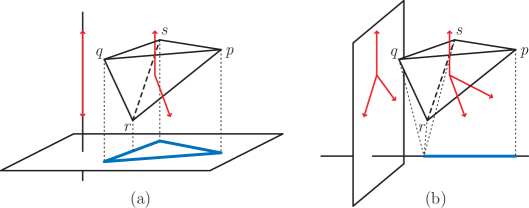
Figure 2. (a) Projection of a tetrahedron onto $\mathbb{R}^{2}$: the edge $pq$ is strictly preserved, while neither the edge $qr$, nor the face qrs, nor the edge qs are (because of conditions (i), (ii) and (iii) respectively). (b) Projection of a tetrahedron to $\mathbb{R}$: only the vertex $p$ is strictly preserved.

The characterization of strictly preserved faces of $P$ uses the normal vectors of the facets of $P$. Let $F_{1},\dots,F_{m}$ denote the facets of $P$. For all $i\in[m]$, let $f_{i}$ denote the normal vector to $F_{i}$, and let $g_{i}\mbox{~{}\raisebox{0.86108pt}{\scriptsize$\mathrm{:}$}$=$ }\tau(f_{i})$. For any face $F$ of $P$, let $\varphi(F)$ denote the set of indices of the facets of $P$ containing $F$, i.e., such that $F=\bigcap_{i\in\varphi(F)}F_{i}$.

Lemma 3.2 (Projection Lemma [AZ99, Zie04]).

A face $F$ of the polytope $P$ is strictly preserved under the projection $\pi$ if and only if $\{g_{i}\ |\ i\in\varphi(F)\}$ is positively spanning. $\Box$

3.1.3. A first construction

Let $t\in\{0,1,\dots,r\}$ be maximal such that the matrices $A_{1},\dots,A_{t}$ are entirely contained in the first $d$ columns of $A$. Let ${\overline{m}}\mbox{~{}\raisebox{0.86108pt}{\scriptsize$\mathrm{:}$}$=$ }\sum_{i=1}^{t}m_{i}$ and ${\overline{n}}\mbox{~{}\raisebox{0.86108pt}{\scriptsize$\mathrm{:}$}$=$ }\sum_{i=1}^{t}n_{i}$. By changing bases appropriately, we can assume that the bottom $n_{i}\times n_{i}$ block of $A_{i}$ is the identity matrix for each $i\geq t+1$. In order to simplify the exposition, we also assume first that ${\overline{n}}=d$, i.e., that the projection on the first $d$ coordinates separates the first $t$ block matrices from the last $r-t$. See Figure 3a.

Let $\{g_{1},\dots,g_{\overline{m}}\}\subset\mathbb{R}^{n-d}$ be a set of vectors such that $G\mbox{~{}\raisebox{0.86108pt}{\scriptsize$\mathrm{:}$}$=$ }\{e_{1},\dots,e_{n-d}\}\cup\{g_{1},\dots,g_{\overline{m}}\}$ is the Gale transform of a full-dimensional simplicial neighborly polytope $Q$ — see [Zie95, Mat02] for definition and properties of Gale duality. By elementary properties of the Gale transform, $Q$ has ${{\overline{m}}+n-d}$ vertices, and $\dim Q=({\overline{m}}+n-d)-(n-d)-1={\overline{m}}-1$. In particular, every subset of $\lfloor\frac{{\overline{m}}-1}{2}\rfloor$ vertices spans a face of $Q$, so every subset of ${\overline{m}}+n-d-\lfloor\frac{{\overline{m}}-1}{2}\rfloor\mbox{~{}$=$\raisebox{0.6458pt}{\scriptsize$\mathrm{:}$} }\alpha$ elements of $G$ is positively spanning.

We deform the matrix $A$ into the matrix $A^{\sim}$ of Figure 3a, using the vectors $g_{1},\dots,g_{\overline{m}}$ to deform the top ${\overline{m}}$ rows. We denote by $P^{\sim}$ the corresponding deformed product. We say that a facet of $P^{\sim}$ is “good” if the right part of the corresponding row of $A^{\sim}$ is covered by a vector of $G$, and “bad” otherwise. Bad facets are hatched in Figure 3a. Observe that there are $\beta\mbox{~{}\raisebox{0.86108pt}{\scriptsize$\mathrm{:}$}$=$ }m-{\overline{m}}-n+d$ bad facets in total.

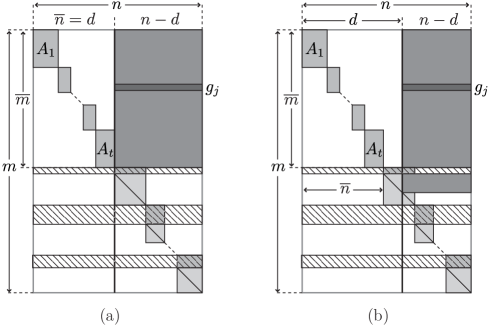
Figure 3. The deformed matrix $A^{\sim}$ (a) when the projection does not slice any block (${\overline{n}}=d$), and (b) when the block $A_{t+1}$ is sliced (${\overline{n}}<d$). Horizontal hatched boxes denote bad row vectors. The top right solid block is formed by the vectors $g_{1},\dots,g_{\overline{m}}$.

Let $F$ be a $k$-face of $P^{\sim}$. Since $P^{\sim}$ is a simple $n$-dimensional polytope, $F$ is the intersection of $n-k$ facets, among which at least $\gamma\mbox{~{}\raisebox{0.86108pt}{\scriptsize$\mathrm{:}$}$=$ }n-k-\beta$ are good facets. If the corresponding elements of $G$ are positively spanning, then $F$ is strictly preserved under projection onto the first $d$ coordinates. Since we have seen that any subset of $\alpha$ vectors of $G$ is positively spanning, $F$ will surely be preserved if $\alpha\leq\gamma$, which is equivalent to

$$k\ \leq\ n-m+\left\lfloor\frac{{\overline{m}}-1}{2}\right\rfloor.$$

Thus, under this assumption, we obtain a $d$-dimensional polytope whose $k$-skeleton is combinatorially equivalent to that of $P\mbox{~{}\raisebox{0.86108pt}{\scriptsize$\mathrm{:}$}$=$ }P_{1}\times\dots\times P_{r}$.

3.1.4. When the projection slices a block

We now discuss the case when ${\overline{n}}<d$, for which the method is very similar. We consider vectors $g_{1},\dots,g_{{\overline{m}}+d-{\overline{n}}}$ such that $G\mbox{~{}\raisebox{0.86108pt}{\scriptsize$\mathrm{:}$}$=$ }\{e_{1},\dots,e_{n-d}\}\cup\{g_{1},\dots,g_{{\overline{m}}+d-{\overline{n}}}\}$ is the Gale dual of a neighborly polytope. We deform the matrix $A$ into the matrix $A^{\sim}$ shown in Figure 3b, using again the vectors $g_{1},\dots,g_{\overline{m}}$ to deform the top ${\overline{m}}$ rows and the vectors $g_{{\overline{m}}+1}\dots,g_{{\overline{m}}+d-{\overline{n}}}$ to deform the top $d-{\overline{n}}$ rows of the $n_{t+1}\times n_{t+1}$ bottom identity submatrix of $A_{t+1}$. This is indeed a valid deformation since we can prescribe the $n_{t+1}\times n_{t+1}$ bottom submatrix of $A_{t+1}$ to be any upper triangular matrix, up to changing the basis appropriately. For the same reasons as before,

1. any subset of at least $\alpha\mbox{~{}\raisebox{0.86108pt}{\scriptsize$\mathrm{:}$}$=$ }{\overline{m}}+n-{\overline{n}}-\left\lfloor\frac{{\overline{m}}+d-{\overline{n}}-1}{2}\right\rfloor$ elements of $G$ is positively spanning;

2. the number of bad facets is $\beta\mbox{~{}\raisebox{0.86108pt}{\scriptsize$\mathrm{:}$}$=$ }m-{\overline{m}}-n+{\overline{n}}$, and thus any $k$-face of $P^{\sim}$ is contained in at least $\gamma\mbox{~{}\raisebox{0.86108pt}{\scriptsize$\mathrm{:}$}$=$ }n-k-\beta$ good facets.

Thus, the condition $\alpha\leq\gamma$ translates to

$$k\ \leq\ n-m+\left\lfloor\frac{{\overline{m}}+d-{\overline{n}}-1}{2}\right\rfloor,$$

and we obtain the following proposition.

Proposition 3.3.

Let $P_{1},\dots,P_{r}$ be simple polytopes of respective dimension $n_{i}$, and with $m_{i}$ many facets. For a fixed integer $d\leq\sum_{i=1}^{r}n_{i}$, let $t$ be maximal such that $\sum_{i=1}^{t}n_{i}\leq d$. Then there exists a $d$-dimensional polytope whose $k$-skeleton is combinatorially equivalent to that of the product $P_{1}\times\dots\times P_{r}$, provided

$$0\ \leq\ k\ \leq\ \sum_{i=1}^{r}(n_{i}-m_{i})+\left\lfloor\frac{1}{2}\left(d-1+\sum_{i=1}^{t}(m_{i}-n_{i})\right)\right\rfloor.\qed$$

In the next two paragraphs, we present two improvements on the bound of this proposition. Both use colorings of the graphs of the polar polytopes $P_{i}^{\triangle}$, in order to weaken the condition $\alpha\leq\gamma$, in two different directions:

1. the first improvement decreases the number of required vectors in the Gale transform $G$, which, in turn, decreases the value of $\alpha$;

2. the second one decreases the number of bad facets, and thus increases the value of $\gamma$.

3.1.5. Multiple vectors

In order to raise our bound on $k$, we can save vectors of $G$ by repeating some of them several times. Namely, any two facets that have no $k$-face in common can share the same vector $g_{j}$. Since any two facets of a simple polytope containing a common $k$-face share a ridge, this condition can be expressed in terms of incidences in the graph of the polar polytope: facets not connected by an edge in this graph can use the same vector $g_{j}$. We denote the chromatic number of a graph $H$ by $\chi(H)$. Then, each $P_{i}$ with $i\leq t$ only contributes $\chi_{i}\mbox{~{}\raisebox{0.86108pt}{\scriptsize$\mathrm{:}$}$=$ }\chi(\text{sk}_{1}P_{i}^{\triangle})$ different vectors in $G$, instead of $m_{i}$ of them. Thus, we only need in total ${\overline{\chi}}\mbox{~{}\raisebox{0.86108pt}{\scriptsize$\mathrm{:}$}$=$ }\sum_{i=1}^{t}\chi_{i}$ different vectors $g_{j}$. This improvement replaces ${\overline{m}}$ by ${\overline{\chi}}$ in the formula of $\alpha$, while $\beta$ and $\gamma$ do not change, and the condition $\alpha\leq\gamma$ is equivalent to

$$k\ \leq\ n-m+{\overline{m}}-{\overline{\chi}}+\left\lfloor\frac{{\overline{\chi}}-d-{\overline{n}}-1}{2}\right\rfloor.$$

Thus, we obtain the following improved proposition:

Proposition 3.4.

Let $P_{1},\dots,P_{r}$ be simple polytopes of respective dimension $n_{i}$, and with $m_{i}$ many facets. Let $\chi_{i}\mbox{~{}\raisebox{0.86108pt}{\scriptsize$\mathrm{:}$}$=$ }\chi(\text{sk}_{1}P_{i}^{\triangle})$ denote the chromatic number of the graph of the polar polytope $P_{i}^{\triangle}$. For a fixed integer $d\leq\sum_{i=1}^{r}n_{i}$, let $t$ be maximal such that $\sum_{i=1}^{t}n_{i}\leq d$. Then there exists a $d$-dimensional polytope whose $k$-skeleton is combinatorially equivalent to that of the product $P_{1}\times\dots\times P_{r}$, provided

$$0\ \leq\ k\ \leq\ \sum_{i=1}^{r}(n_{i}-m_{i})+\sum_{i=1}^{t}(m_{i}-\chi_{i})+\left\lfloor\frac{1}{2}\left(d-1+\sum_{i=1}^{t}(\chi_{i}-n_{i})\right)\right\rfloor.\qed$$

Example 3.5.

Since polars of simple polytopes are simplicial, $\chi_{i}\geq n_{i}$ is an obvious lower bound for the chromatic number of the dual graph of $P_{i}$. Polytopes that attain this lower bound with equality are characterized by the property that all their $2$-dimensional faces have an even number of vertices, and are called even polytopes.

If all $P_{i}$ are even polytopes, then ${\overline{n}}={\overline{\chi}}$, and we obtain a $d$-dimensional polytope with the same $k$-skeleton as $P_{1}\times\dots\times P_{r}$ provided

$$k\ \leq\ n-m+{\overline{m}}-{\overline{n}}+\left\lfloor\frac{d-1}{2}\right\rfloor.$$

In order to maximize $k$, we should maximize ${\overline{m}}-{\overline{n}}$, subject to the condition ${\overline{n}}\leq d$. For example, if all $n_{i}$ are equal, this amounts to ordering the $P_{i}$ by decreasing number of facets.

3.1.6. Scaling blocks

We can also apply colorings to the blocks $A_{i}$ with $i\geq t+1$, by filling in the area below $G$ and above the diagonal blocks. To explain this, assume for the moment that $\chi_{i}\leq n_{i+1}$ for a certain fixed $i\geq t+2$. Assume that the rows of $A_{i}$ are colored with $\chi_{i}$ colors using a valid coloring $c:[m_{i}]\to[\chi_{i}]$ of the graph of the polar polytope $P_{i}^{\triangle}$. Let $\Gamma$ be the incidence matrix of $c$, defined by $\Gamma_{j,k}=1$ if $c(j)=k$, and $\Gamma_{j,k}=0$ otherwise. Thus, $\Gamma$ is a matrix of size $m_{i}\times\chi_{i}$. We put this matrix to the right of $A_{i}$ and above $A_{i+1}$ as in Figure 4b, so that we append the same unit vector to each row of $A_{i}$ in the same color class. Moreover, we scale all entries of the block $A_{i}$ by a sufficiently small constant $\varepsilon>0$.

Figure 4. How to raise the dimension of the preserved skeleton by inserting the incidence matrix $\Gamma$ of a coloring of the graph of the polar polytope $P_{i}^{\triangle}$. Part (a) shows the situation before the insertion of $\Gamma$, and part (b) the changes that have occurred. Bad row vectors and unnecessary columns are hatched. The entries in the matrix to the left of $\Gamma$ must be rescaled to retain a valid inequality description of $P$.

In this setting, the situation is slightly different:

1. In the Gale dual $G$, we do not need the $n_{i}$ basis vectors of $\mathbb{R}^{n-d}$ hatched in Figure 4b. Let $a\mbox{~{}\raisebox{0.86108pt}{\scriptsize$\mathrm{:}$}$=$ }\sum_{j<i}n_{j}$ denote the index of the last column vector of $A_{i-1}$ and $b\mbox{~{}\raisebox{0.86108pt}{\scriptsize$\mathrm{:}$}$=$ }1+\sum_{j\leq i}n_{j}$ denote the index of the first column vector of $A_{i+1}$. We define $G\mbox{~{}\raisebox{0.86108pt}{\scriptsize$\mathrm{:}$}$=$ }\{e_{1},\dots,e_{a-d},e_{b-d},\dots,e_{n-d}\}\cup\{g_{1},\dots,g_{\overline{m}}\}$ to be the Gale transform of a simplicial neighborly polytope $Q$ of dimension ${\overline{m}}-1-n_{i}$. As before, any subset of $\alpha\mbox{~{}\raisebox{0.86108pt}{\scriptsize$\mathrm{:}$}$=$ }{\overline{m}}+n-{\overline{n}}-n_{i}-\lfloor\frac{{\overline{m}}+d-{\overline{n}}-n_{i}-1}{2}\rfloor$ vectors of $G$ positively spans $\mathbb{R}^{n-d}$.

2. “Bad” facets are defined as before, except that the top $m_{i}-n_{i}$ rows of $A_{i}$ are not bad anymore, but all of the first $m_{i+1}-n_{i+1}+\chi_{i}$ rows of $A_{i+1}$ are now bad. Thus, the net change in the number of bad rows is $\chi_{i}-m_{i}+n_{i}$, so that any $k$-face is contained in at least $\gamma\mbox{~{}\raisebox{0.86108pt}{\scriptsize$\mathrm{:}$}$=$ }2n-k-m+{\overline{m}}-{\overline{n}}+m_{i}-n_{i}-\chi_{i}$ good rows. Up to $\varepsilon$-entry elements, the last $n-d$ coordinates of these rows correspond to pairwise distinct elements of $G$.

Applying the same reasoning as above, the $k$-skeleton of $P^{\sim}$ is strictly preserved under projection to the first $d$ coordinates as soon as $\alpha\leq\gamma$, which is equivalent to

$$k\ \leq\ n-m+m_{i}-\chi_{i}+\left\lfloor\frac{{\overline{m}}+d-{\overline{n}}-n_{i}-1}{2}\right\rfloor.$$

Thus, we improve our bound on $k$ provided

$$\Delta\mbox{~{}\raisebox{0.86108pt}{\scriptsize$\mathrm{:}$}$=$ }m_{i}-\chi_{i}+\left\lfloor\frac{{\overline{m}}+d-{\overline{n}}-n_{i}-1}{2}\right\rfloor-\left\lfloor\frac{{\overline{m}}+d-{\overline{n}}-1}{2}\right\rfloor>0.$$

For example, this difference $\Delta$ is big for polytopes whose polars have many vertices but a small chromatic number.

Finally, observe that one can apply this “scaling” improvement even if $\chi_{i}>n_{i+1}$ (except that it will perturb more than the two blocks $A_{i}$ and $A_{i+1}$) and to more than one matrix $A_{i}$. Please see the example in Figure 5. In this picture, the $\Gamma$ blocks are incidence matrices of colorings of the graphs of the polar polytopes. Call “diagonal entries” all entries on the diagonal of the $n_{i}\times n_{i}$ bottom submatrix of a factor $A_{i}$. A column is unnecessary (hatched in the picture) if its diagonal entry has a $\Gamma$ block on the right and no $\Gamma$ block above. Good rows are those covered by a vector $g_{j}$ or a $\Gamma$ block, together with the basis vectors whose diagonal entry has no $\Gamma$ block above (bad rows are hatched in the picture).

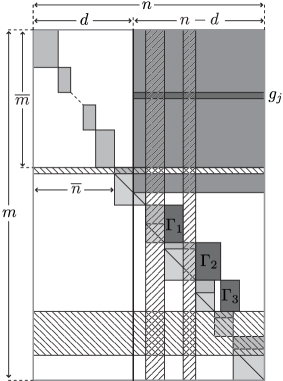
Figure 5. How to reduce the number of vectors in the Gale transform using various coloring matrices of polar polytopes. Situations where $\chi_{i}>n_{i+1}$ can be accommodated for as illustrated by the matrix $\Gamma_{2}$ in the picture.

Example 3.6.

1. If $P_{i}$ is a segment, then $n_{i}=1$, $m_{i}=2$ and $\chi_{i}=1$, so that $\Delta=1$ if ${\overline{m}}$ is even and $0$ otherwise. Iterating this, if $P_{i}$ is an $s$-dimensional cube, then $\Delta\simeq\frac{s}{2}$. This yields neighborly cubical polytopes — see [JZ00, JS07].

2. If $P_{i}$ is an even cycle, then $n_{i}=2$, $m_{i}=2p$ and $\chi_{i}=2$, so that $\Delta=2p-3$. This yields projected products of polygons — see [Zie04, SZ09].

In general, it is difficult to give the explicit ordering of the factors and choice of deformation that will yield the largest possible value of $k$ attainable by a concrete product $P_{1}\times\dots\times P_{r}$ of simple polytopes, and consequently to summarize this improvement by a precise proposition as we did for our first improvement. However, this best value can clearly be found by optimizing over the finite set of all possible orderings and types of deformation. Furthermore, we can be much more explicit for products of simplices, as we detail in the next section.

3.2. Projection of deformed product of simplices

We are now ready to apply this general construction to the particular case of products of simplices. For this, we represent the simplex $\triangle_{n_{i}}$ by the inequality system $A_{i}x\leq b_{i}$, where

$$A_{i}\ \mbox{~{}\raisebox{0.86108pt}{\scriptsize$\mathrm{:}$}$=$ }\ \begin{pmatrix}-1&\dots&-1\\ 1\\ &\ddots\\ &&1\end{pmatrix}$$

and $b_{i}$ is a suitable right-hand side. We express the results of the construction with a case distinction according to the number $s\mbox{~{}\raisebox{0.86108pt}{\scriptsize$\mathrm{:}$}$=$ }|\{i\in[r]\ |\ n_{i}=1\}|$ of segments in the product $\triangle_{\underline{n}}$.

Proposition 3.7.

Let $\underline{n}\mbox{~{}\raisebox{0.86108pt}{\scriptsize$\mathrm{:}$}$=$ }(n_{1},\dots,n_{r})$ with $1=n_{1}=\dots=n_{s}<n_{s+1}\leq\dots\leq n_{r}$. Then

1. for any $0\leq d\leq s-1$, there exists a $d$-dimensional $(k,\underline{n})$-PPSN polytope provided

   $$k\ \leq\ \left\lfloor\frac{d}{2}\right\rfloor-r+s-1.$$

2. for any $s\leq d\leq n$, there exists a $d$-dimensional $(k,\underline{n})$-PPSN polytope provided

   $$k\ \leq\ \left\lfloor\frac{d+t-s}{2}\right\rfloor-r+s.$$

   where $t\in\{s,\dots,r\}$ denotes the maximal integer such that $\sum_{i=1}^{t}n_{i}\leq d$.

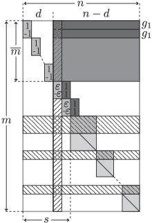
Figure 6. How to obtain PPSN polytopes from a deformed product construction, when the number $s$ of segment factors exceeds the target dimension $d$ of the projection.

Proof of (1).

This is a special case of the results obtainable with the methods of Section 3.1. The best construction is obtained using the matrix in Figure 6, from which we read off that

1. any subset of at least $\alpha\mbox{~{}\raisebox{0.86108pt}{\scriptsize$\mathrm{:}$}$=$ }n-\left\lfloor\frac{d}{2}\right\rfloor$ vectors in $G$ is positively spanning; and

2. the number of bad facets is $\beta\mbox{~{}\raisebox{0.86108pt}{\scriptsize$\mathrm{:}$}$=$ }r-s+1$, and therefore any $k$-face of $P^{\sim}$ is contained in at least $\gamma\mbox{~{}\raisebox{0.86108pt}{\scriptsize$\mathrm{:}$}$=$ }n-k-r+s-1$ good facets.

From this, the claim follows. ∎

Proof of (2).

Consider the deformed product of Figure 7a. Using similar calculations as before, we deduce that

1. any subset of at least $\alpha\mbox{~{}\raisebox{0.86108pt}{\scriptsize$\mathrm{:}$}$=$ }t-s+n-\left\lfloor\frac{d+t-s-1}{2}\right\rfloor$ vectors in $G$ is positively spanning; and

2. the number of bad facets is $\beta\mbox{~{}\raisebox{0.86108pt}{\scriptsize$\mathrm{:}$}$=$ }r-t$, and therefore any $k$-face of $P^{\sim}$ is contained in at least $\gamma\mbox{~{}\raisebox{0.86108pt}{\scriptsize$\mathrm{:}$}$=$ }n-k-r+t$ good facets.

This yields a bound of

$$k\ \leq\ \left\lfloor\frac{d+t-s-1}{2}\right\rfloor-r+s.$$

We optimize the final ‘$-1$’ away by suitably deforming the matrix $A_{t+1}$ as in Figure 7b. This amounts to adding one more vector $g_{\star}$ to the Gale diagram, so that the first row of $A_{t+1}$ ceases to be a bad facet. This deformation is valid because:

1. the matrix

   $$\begin{pmatrix}-1&\dots&-1&\star&\dots&\star\\ M\\ &\ddots\\ &&M\\ &&&1\\ &&&&\ddots\\ &&&&&1\end{pmatrix}$$

   still defines a simplex, as long as the ‘$\star$’ entries are negative and $M\gg 0$ is chosen to be sufficiently large;

2. we can in fact choose the new vector $g_{\star}$ to have only negative entries, by imposing an additional restriction on the Gale diagram $G=\{e_{1},\dots,e_{n-d}$, $g_{1},\dots,g_{d+t},g_{\star}\}$ of $Q$. Namely, we require that the vertices of the $(d+t)$-dimensional simplicial polytope $Q$ that correspond to the Gale vectors $g_{1},\dots,g_{d+t}$ lie on a facet. This forces the remaining vectors $e_{1},\dots,e_{n-d},g_{\star}$ to be positively spanning, so that $g_{\star}$ has only negative entries. ∎

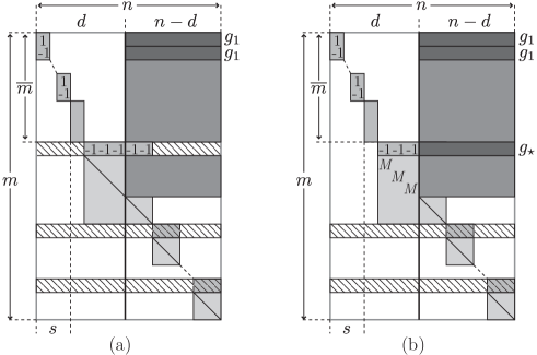
Figure 7. Obtaining PPSN polytopes from a deformed product construction, when few of the factors are segments. Part (a) shows the technique used so far, and part (b) an additional optimization that exchanges a bad facet for a new vector in the Gale transform.

Finally, we reformulate Proposition 3.7 to express, in terms of $k$ and $\underline{n}\mbox{~{}\raisebox{0.86108pt}{\scriptsize$\mathrm{:}$}$=$ }(n_{1},\dots,n_{r})$, what dimensions a $(k,\underline{n})$-PPSN polytope can have. This yields upper bounds on $\delta_{pr}(k,\underline{n})$.

Theorem 3.8.

For any $k\geq 0$ and $\underline{n}\mbox{~{}\raisebox{0.86108pt}{\scriptsize$\mathrm{:}$}$=$ }(n_{1},\dots,n_{r})$ with ${1=n_{1}=\dots=n_{s}<n_{s+1}\leq\dots\leq n_{r}}$,

$$\delta_{pr}(k,\underline{n})\ \leq\ \begin{cases}2(k+r)-s-t&\text{if }3s\leq 2k+2r,\\ 2(k+r-s)+1&\text{if }3s=2k+2r+1,\\ 2(k+r-s+1)&\text{if }3s\geq 2k+2r+2,\end{cases}$$

where $t\in\{s,\dots,r\}$ is maximal such that

$$3s+\sum_{i=s+1}^{t}(n_{i}+1)\ \leq\ 2k+2r.$$

Proof.

Apply part (1) of Proposition 3.7 when $3s\geq 2k+2r+2$ and part (2) otherwise. ∎

Remark 3.9.

When all the $n_{i}$’s are large compared to $k$, the dimension of the $(k,\underline{n})$-PPSN polytope provided by this theorem is bigger than the dimension $2k+r+1$ of the $(k,\underline{n})$-PPSN polytope obtained by the Minkowski sum of cyclic polytopes of Theorem 2.6. However, if we have many segments (neighborly cubical polytopes), or more generally if many $n_{i}$’s are small compared to $k$, this construction provides our best examples of PPSN polytopes.

4. Topological Obstructions

In this section, we give lower bounds on the minimal dimension $\delta_{pr}(k,\underline{n})$ of a $(k,\underline{n})$-PPSN polytope, applying and extending a method developed by Sanyal [San09] to bound the number of vertices of Minkowski sums of polytopes. This method provides lower bounds on the target dimension of any linear projection that preserves a given set of faces of a polytope. It uses Gale duality to associate a certain simplicial complex $\mathcal{K}$ to the set of faces that are preserved under the projection. Then lower bounds on the embeddability dimension of $\mathcal{K}$ transfer to lower bounds on the target dimension of the projection. In turn, the embeddability dimension is bounded via colorings of the Kneser graph of the system of minimal non-faces of $\mathcal{K}$, using Sarkaria’s Embeddability Theorem.

For the convenience of the reader, we first quickly recall this embeddability criterion. We then provide a brief overview of Sanyal’s method before applying it to obtain lower bounds on the dimension of $(k,\underline{n})$-PPSN polytopes. As mentioned in the introduction, these bounds match the upper bounds obtained from our different constructions for a wide range of parameters, and thus give the exact value of the minimal dimension of a PPSN polytope.

4.1. Sarkaria’s embeddability criterion

4.1.1. Kneser graphs

Recall that a $k$-coloring of a graph $G=(V,E)$ is a map $c:V\to[k]$ such that $c(u)\neq c(v)$ for $(u,v)\in E$. As usual, let $\chi(G)$ denote the chromatic number of $G$ (i.e., the minimal $k$ such that $G$ admits a $k$-coloring). We are interested in the chromatic number of so-called Kneser graphs.

Let $\mathcal{Z}$ be a subset of the power set $2^{[n]}$ of $[n]$. The Kneser graph on $\mathcal{Z}$, denoted $\mathrm{KG}(\mathcal{Z})$, is the graph with vertex set $\mathcal{Z}$, where $X,Y\in\mathcal{Z}$ are adjacent if and only if $X\cap Y=\emptyset$:

$$\mathrm{KG}(\mathcal{Z})\ \mbox{~{}\raisebox{0.86108pt}{\scriptsize$\mathrm{:}$}$=$ }\ \left(\mathcal{Z},\{(X,Y)\in\mathcal{Z}^{2}\ |\ X\cap Y=\emptyset\}\right).$$

Let $\mathrm{KG}_{n}^{k}\mbox{~{}\raisebox{0.86108pt}{\scriptsize$\mathrm{:}$}$=$ }\mathrm{KG}\big{(}{[n]\choose k}\big{)}$ denote the Kneser graph on the set of subsets of $[n]$ of size $k$. For example, the graph $\mathrm{KG}_{n}^{1}$ is the complete graph $K_{n}$ (of chromatic number $n$) and the graph $\mathrm{KG}_{5}^{2}$ is the Petersen graph (of chromatic number $3$).

Remark 4.1.

1. If $n\leq 2k-1$, then any two $k$-subsets of $[n]$ intersect and the Kneser graph $\mathrm{KG}_{n}^{k}$ is independent (i.e., it has no edge). Thus its chromatic number is $\chi(\mathrm{KG}_{n}^{k})=1$.

2. If $n\geq 2k-1$, then $\chi(\mathrm{KG}_{n}^{k})\leq n-2k+2$. Indeed, the map $c:{[n]\choose k}\to[n-2k+2]$ defined by $c(F)\mbox{~{}\raisebox{0.86108pt}{\scriptsize$\mathrm{:}$}$=$ }\min(F\cup\{n-2k+2\})$ is a $(n-2k+2)$-coloring of $\mathrm{KG}_{n}^{k}$.

In fact, it turns out that this upper bound is the exact chromatic number of the Kneser graph: $\chi(\mathrm{KG}_{n}^{k})=\max\{1,n-2k+2\}$. This result was conjectured by Kneser [Kne55] in 1955, and proved by Lovász [Lov78] in 1978 applying the Borsuk-Ulam Theorem — see [Mat03] for more details. However, we will only need the upper bound for the topological obstruction.

4.1.2. Sarkaria’s Theorem

Our lower bounds on the dimension of $(k,\underline{n})$-PPSN polytopes rely on lower bounds for the dimension in which certain simplicial complexes can be embedded. Among other possible methods [Mat03], we use Sarkaria’s Coloring and Embedding Theorem.

We associate to any simplicial complex $\mathcal{K}$ the set system $\mathcal{Z}$ of minimal non-faces of $\mathcal{K}$, that is, the inclusion-minimal sets of $2^{V(\mathcal{K})}\smallsetminus\mathcal{K}$. For example, the complex of minimal non-faces of the $k$-skeleton of the $n$-dimensional simplex is ${[n+1]\choose k+2}$. Sarkaria’s Theorem provides a lower bound on the dimension into which $\mathcal{K}$ can be embedded, in terms of the chromatic number of the Kneser graph of $\mathcal{Z}$.

Theorem 4.2 (Sarkaria’s Theorem).

Let $\mathcal{K}$ be a simplicial complex embeddable in $\mathbb{R}^{d}$, $\mathcal{Z}$ be the system of minimal non-faces of $\mathcal{K}$, and $\mathrm{KG}(\mathcal{Z})$ be the Kneser graph on $\mathcal{Z}$. Then

$$d\ \geq\ |V(\mathcal{K})|-\chi(\mathrm{KG}(\mathcal{Z}))-1.$$

In other words, we get large lower bounds on the possible embedding dimension of $\mathcal{K}$ when the Kneser graph of minimal non-faces of $\mathcal{K}$ has small chromatic number. We refer to the excellent treatment in [Mat03] for further details.

4.2. Sanyal’s topological obstruction method

For given integers $n>d$, we consider the orthogonal projection $\pi:\mathbb{R}^{n}\to\mathbb{R}^{d}$ to the first $d$ coordinates, and its dual projection $\tau:\mathbb{R}^{n}\to\mathbb{R}^{n-d}$ to the last $n-d$ coordinates. Let $P$ be a full-dimensional simple polytope in $\mathbb{R}^{n}$, with $0$ in its interior, and assume that its vertices are strictly preserved under $\pi$. Let $F_{1},\dots,F_{m}$ denote the facets of $P$. For all $i\in[m]$, let $f_{i}$ denote the normal vector to $F_{i}$, and let $g_{i}\mbox{~{}\raisebox{0.86108pt}{\scriptsize$\mathrm{:}$}$=$ }\tau(f_{i})$. For any face $F$ of $P$, let $\varphi(F)$ denote the set of indices of the facets of $P$ containing $F$, i.e., such that $F=\bigcap_{i\in\varphi(F)}F_{i}$.

Lemma 4.3 (Sanyal [San09]).

The vector configuration $G\mbox{~{}\raisebox{0.86108pt}{\scriptsize$\mathrm{:}$}$=$ }\{g_{i}\ |\ i\in[m]\}\subset\mathbb{R}^{n-d}$ is the Gale transform of the vertex set $\{a_{i}\ |\ i\in[m]\}$ of a (full-dimensional) polytope $Q$ of $\mathbb{R}^{m-n+d-1}$. Up to a slight perturbation of the facets of $P$, we can even assume $Q$ to be simplicial.

We will refer to the polytope $Q$ as Sanyal’s projection polytope. The faces of this polytope capture the key notion of strictly preserved faces of $P$ — remember Definition 3.1. Indeed, the Projection Lemma 3.2 ensures that for any face $F$ of $P$ that is strictly preserved by the projection $\pi$, the set $\{g_{i}\ |\ i\in\varphi(F)\}$ is positively spanning. By Gale duality, this implies that the set of vertices $\{a_{i}\ |\ i\in[m]\smallsetminus\varphi(F)\}$ forms a face of $Q$.

Example 4.4.

Let $P$ be a triangular prism in $3$-space that projects to a hexagon as in Figure 8a, so that $n=3$, $d=2$ and $m=5$. The vector configuration $G\subset\mathbb{R}^{1}$ obtained by projecting $P$’s normal vectors consists of three vectors pointing up and two pointing down, so that Sanyal’s projection polytope $Q$ is a bipyramid over a triangle. An edge $F_{i}\cap F_{j}$ of $P$ that is preserved under projection corresponds to the face $[5]\smallsetminus\{i,j\}$ of $Q$. Notice that the six faces of $Q$ corresponding to the six edges of $P$ that are preserved under projection (in bold in Figure 8a) make up the entire boundary complex of the bipyramid $Q$.

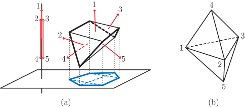
Figure 8. (a) Projection of a triangular prism and (b) its associated projection polytope $Q$. The six faces of $Q$ corresponding to the six edges of $P$ preserved under projection (bold) make up the entire boundary complex of $Q$.

Let $\mathcal{F}$ be a collection of faces of $P$ that are strictly preserved under $\pi$. Define $\mathcal{K}$ to be the simplicial complex induced by $\{[m]\smallsetminus\varphi(F)\ |\ F\in\mathcal{F}\}$.

Remark 4.5.

Notice that not all non-empty faces of $\mathcal{K}$ correspond to non-empty faces in $\mathcal{F}$: in Example 4.4, if $\mathcal{F}$ consists of all strictly preserved edges, then $\mathcal{K}$ is the entire boundary complex of Sanyal’s projection polytope $Q$, so that it contains the edge $\{2,3\}$. But then the complementary intersection of facets, $F_{1}\cap F_{4}\cap F_{5}$, does not correspond to any non-empty face of $P$.

Since the set of vertices $\{a_{i}\ |\ i\in[m]\smallsetminus\varphi(F)\}$ forms a face of $Q$ for any face $F\in\mathcal{F}$, and since $Q$ is simplicial, $\mathcal{K}$ is a subcomplex of the face complex of $Q\subset\mathbb{R}^{m-n+d-1}$. In particular, when $\mathcal{K}$ is not the entire boundary complex of $Q$, it embeds into $\mathbb{R}^{m-n+d-2}$ by stereographic projection (otherwise, it only embeds into $\mathbb{R}^{m-n+d-1}$, as happens in Example 4.4).

Thus, given the simple polytope $P\subset\mathbb{R}^{n}$ and a set $\mathcal{F}$ of faces of $P$ that we want to preserve under projection, the study of the embeddability of the corresponding abstract simplicial complex $\mathcal{K}$ provides lower bounds on the dimension $d$ in which we can project $P$. We proceed in the following way:

1. we first choose our subset $\mathcal{F}$ of strictly preserved faces to be simple enough to understand and large enough to provide an obstruction;

2. we then understand the system $\mathcal{Z}$ of minimal non-faces of the simplicial complex $\mathcal{K}$;

3. finally, we find a suitable coloring of the Kneser graph on $\mathcal{Z}$ and apply Sarkaria’s Theorem 4.2 to bound the dimension in which $\mathcal{K}$ can be embedded: a $t$-coloring of $\mathrm{KG}(\mathcal{Z})$ ensures that $\mathcal{K}$ is not embeddable into $|V(\mathcal{K})|-t-2=m-t-2$, which by the previous paragraph bounds the dimension $d$ from below as follows:

Theorem 4.6 (Sanyal [San09]).

Let $P$ be a simple polytope in $\mathbb{R}^{n}$ whose facets are in general position, and let $\pi:\mathbb{R}^{n}\to\mathbb{R}^{d}$ be a projection. Let $\mathcal{F}$ be a subset of the set of all strictly preserved faces of $P$ under $\pi$, let $\mathcal{K}$ be the simplicial complex induced by $\{[m]\smallsetminus\varphi(F)\ |\ F\in\mathcal{F}\}$, and let $\mathcal{Z}$ be its system of minimal non-faces. If the Kneser graph $\mathrm{KG}(\mathcal{Z})$ is $t$-colorable, then

1. if $\mathcal{K}$ is not the entire boundary complex of the Sanyal polytope $Q$, then $d\geq n-t+1$;

2. otherwise, $d\geq n-t$. $\Box$

In the remainder of this section, we apply Sanyal’s topological obstruction to our problem. The hope was initially to extend it to bound the target dimension of a projection preserving the $k$-skeleton of an arbitrary product of simple polytopes. However, the combinatorics involved to deal with this general question turn out to be too complicated, and so we restrict our attention to products of simplices. This yields bounds on the minimal dimension $\delta_{pr}(k,\underline{n})$ of a $(k,\underline{n})$-PPSN polytope.

4.3. Preserving the $k$-skeleton of a product of simplices

In this section, we understand the abstract simplicial complex $\mathcal{K}$ corresponding to our problem, and describe its system of minimal non-faces.

The facets of $\triangle_{\underline{n}}$ are exactly the products

$$\psi_{i,j}\ \mbox{~{}\raisebox{0.86108pt}{\scriptsize$\mathrm{:}$}$=$ }\ \triangle_{n_{1}}\times\dots\times\triangle_{n_{i-1}}\times(\triangle_{n_{i}}\smallsetminus\{j\})\times\triangle_{n_{i+1}}\times\dots\times\triangle_{n_{r}},$$

for $i\in[r]$ and $j\in[n_{i}+1]$. We identify the facet $\psi_{i,j}$ with the element $j\in[n_{i}+1]$ of the disjoint union $[n_{1}+1]\uplus[n_{2}+1]\uplus\dots\uplus[n_{r}+1]$.

Let $F\mbox{~{}\raisebox{0.86108pt}{\scriptsize$\mathrm{:}$}$=$ }F_{1}\times\dots\times F_{r}$ be a $k$-face of $\triangle_{\underline{n}}$. Then $F$ is contained in a facet $\psi_{i,j}$ of $\triangle_{\underline{n}}$ if and only if $j\notin F_{i}$. Thus, the set of facets of $\triangle_{\underline{n}}$ that do not contain $F$ is exactly ${F_{1}\uplus\dots\uplus F_{r}}$. Consequently, if we want to preserve the $k$-skeleton of $\triangle_{\underline{n}}$, then the abstract simplicial complex $\mathcal{K}$ we are interested in is induced by

(3) $$\bigg{\{}F_{1}\uplus\dots\uplus F_{r}\ \big{|}\ \emptyset\neq F_{i}\subset[n_{i}+1]\text{ for all }i\in[r],\textrm{ and }\sum_{i\in[r]}(|F_{i}|-1)=k\bigg{\}}.$$

Remark 4.7.

In contrast to the general case, when we want to preserve the complete $k$-skeleton of a product of simplices, the complex $\mathcal{K}$ cannot be the entire boundary complex of the Sanyal polytope $Q$. As a consequence, the better lower bound from part (1) of Sanyal’s Theorem 4.6 always holds, and we always use it from now on without further notice.

To prove that $\mathcal{K}$ cannot cover the entire boundary complex of $Q$, observe that

$$\dim Q\ =\ m-n+d-1\ =\ \sum(n_{i}+1)-\sum n_{i}+d-1\ =\ r+d-1,$$

while $\dim\mathcal{K}=r+k-1$ by (3). A necessary condition for $\mathcal{K}$ to be the entire boundary complex of $Q$ is that $\dim\mathcal{K}=\dim Q-1$, which translates to $d=k+1$. Now suppose that the entire $k$-skeleton of $\triangle_{\underline{n}}$ is preserved under projection to dimension $k+1$. Then the projections of those $k$-faces are facets of $\pi(\triangle_{\underline{n}})$. Since any ridge of the projected polytope is contained in exactly two facets, and the entire $k$-skeleton of $\triangle_{\underline{n}}$ is preserved, we know that any $(k-1)$-face of $\triangle_{\underline{n}}$ is also contained in exactly two $k$-faces. But this can only happen if $k=n-1$, which means $n=d$.

Recall from Example 4.4 that $\mathcal{K}$ can be the entire boundary complex of $Q$ if we do not preserve all $k$-faces of $\triangle_{\underline{n}}$.

The following lemma gives a description of the minimal non-faces of $\mathcal{K}$:

Lemma 4.8.

The system of minimal non-faces of $\mathcal{K}$ is

$$\mathcal{Z}\ \mbox{~{}\raisebox{0.86108pt}{\scriptsize$\mathrm{:}$}$=$ }\ \bigg{\{}G_{1}\uplus\dots\uplus G_{r}\ \big{|}\ |G_{i}|\neq 1\text{ for all }i\in[r],\textrm{ and }\sum_{i\,|\,G_{i}\neq\emptyset}(|G_{i}|-1)=k+1\bigg{\}}.$$

Proof.

A subset $G\mbox{~{}\raisebox{0.86108pt}{\scriptsize$\mathrm{:}$}$=$ }G_{1}\uplus\dots\uplus G_{r}$ of $[n_{1}+1]\uplus[n_{2}+1]\uplus\dots\uplus[n_{r}+1]$ is a face of $\mathcal{K}$ when it can be extended to a subset $F_{1}\uplus\dots\uplus F_{r}$ with $\sum(|F_{i}|-1)=k$ and $\emptyset\neq F_{i}\subset[n_{i}+1]$ for all $i\in[r]$, that is, when

$$k\ \geq\ \left|\big{\{}i\in[r]\ |\ G_{i}=\emptyset\big{\}}\right|+\sum_{i\in[r]}(|G_{i}|-1)=\sum_{i\,|\,G_{i}\neq\emptyset}(|G_{i}|-1).$$

Thus, $G$ is a non-face if and only if

$$\sum_{i\,|\,G_{i}\neq\emptyset}(|G_{i}|-1)\ \geq\ k+1.$$

If $\sum_{i\,|\,G_{i}\neq\emptyset}(|G_{i}|-1)>k+1$, then removing any element provides a smaller non-face. If there is an $i$ such that $|G_{i}|=1$, then removing the unique element of $G_{i}$ provides a smaller non-face. Thus, if $G$ is a minimal non-face, then $\sum_{i\,|\,G_{i}\neq\emptyset}(|G_{i}|-1)=k+1$, and $|G_{i}|\neq 1$ for all $i\in[r]$.

Reciprocally, if $G$ is a non-minimal non-face, then it is possible to remove one element keeping a non-face. Let $i\in[r]$ be such that we can remove one element from $G_{i}$, keeping a non-face. Then, either $|G_{i}|=1$, or

$$\sum_{j\,|\,G_{j}\neq\emptyset}(|G_{j}|-1)\ \geq\ 1+(|G_{i}|-2)+\sum_{j\neq i\,|\,G_{j}\neq\emptyset}(|G_{j}|-1)\geq k+2,$$

since we keep a non-face. ∎

4.4. Colorings of $\mathrm{KG}(\mathcal{Z})$

Our next goal is to provide a suitable coloring of the Kneser graph on the system $\mathcal{Z}$ of minimal non-faces of $\mathcal{K}$. Let $S\mbox{~{}\raisebox{0.86108pt}{\scriptsize$\mathrm{:}$}$=$ }\{i\in[r]\ |\ n_{i}=1\}$ denote the set of indices corresponding to the segments, and $R\mbox{~{}\raisebox{0.86108pt}{\scriptsize$\mathrm{:}$}$=$ }\{i\in[r]\ |\ n_{i}\geq 2\}$ the set of indices corresponding to the non-segments in the product $\triangle_{\underline{n}}$. We first provide a coloring for two extremal situations.

Theorem 4.9 (Topological obstruction for low-dimensional skeleta).

If $k\leq\sum_{i\in R}\left\lfloor\frac{n_{i}-2}{2}\right\rfloor$, then the dimension of any $(k,\underline{n})$-PPSN polytope cannot be smaller than $2k+|R|+1$:

$$\delta_{pr}(k,\underline{n})\ \geq\ 2k+|R|+1.$$

Proof.

Let $k_{1},\dots,k_{r}\in\mathbb{N}$ be such that

$$\sum_{i\in[r]}k_{i}\ =\ k\quad\textrm{and}\quad\begin{cases}k_{i}=0&\textrm{for }i\in S;\\ 0\leq k_{i}\leq\frac{n_{i}-2}{2}&\textrm{for }i\in R.\end{cases}$$

Observe that

1. such a tuple exists since $k\leq\sum_{i\in R}\left\lfloor\frac{n_{i}-2}{2}\right\rfloor$, and

2. for any minimal non-face $G\mbox{~{}\raisebox{0.86108pt}{\scriptsize$\mathrm{:}$}$=$ }G_{1}\uplus\dots\uplus G_{r}$ of $\mathcal{Z}$, there exists $i\in[r]$ such that $|G_{i}|\geq k_{i}+2$. Indeed, if $|G_{i}|\leq k_{i}+1$ for all $i\in[r]$, then

   $$k+1\ =\ \sum_{i\,|\,G_{i}\neq\emptyset}(|G_{i}|-1)\ \leq\ \sum_{i\,|\,G_{i}\neq\emptyset}k_{i}\ \leq\ \sum_{i\in[r]}k_{i}\ =\ k,$$

   which is impossible.

For all $i\in[r]$, we fix a proper coloring $\gamma_{i}:{[n_{i}+1]\choose[k_{i}+2]}\to[\chi_{i}]$ of the Kneser graph $\mathrm{KG}_{n_{i}+1}^{k_{i}+2}$, with $\chi_{i}=1$ if $i\in S$ and $\chi_{i}=n_{i}-2k_{i}-1$ if $i\in R$ — see Section 4.1.1. We define a coloring $\gamma:\mathcal{Z}\to[\chi_{1}]\uplus\dots\uplus[\chi_{r}]$ of the Kneser graph on $\mathcal{Z}$ as follows. Let $G\mbox{~{}\raisebox{0.86108pt}{\scriptsize$\mathrm{:}$}$=$ }G_{1}\uplus\dots\uplus G_{r}$ be a given minimal non-face of $\mathcal{Z}$. We arbitrarily choose an $i\in[r]$ such that $|G_{i}|\geq k_{i}+2$, and a subset $g$ of $G_{i}$ with $k_{i}+2$ elements. We color $G$ with the color of $g$ in $\mathrm{KG}_{n_{i}+1}^{k_{i}+2}$, that is, we define $\gamma(G)\mbox{~{}\raisebox{0.86108pt}{\scriptsize$\mathrm{:}$}$=$ }\gamma_{i}(g)$.

The coloring $\gamma$ is a proper coloring of the Kneser graph $\mathrm{KG}(\mathcal{Z})$. Indeed, let $G\mbox{~{}\raisebox{0.86108pt}{\scriptsize$\mathrm{:}$}$=$ }G_{1}\uplus\dots\uplus G_{r}$ and $H\mbox{~{}\raisebox{0.86108pt}{\scriptsize$\mathrm{:}$}$=$ }H_{1}\uplus\dots\uplus H_{r}$ be two minimal non-faces of $\mathcal{Z}$ related by an edge in $\mathrm{KG}(\mathcal{Z})$, which means that they do not intersect. Let $i\in[r]$ and $g\subset G_{i}$ be such that we have colored $G$ with $\gamma_{i}(g)$, and similarly $j\in[r]$ and $h\subset G_{j}$ be such that we have colored $H$ with $\gamma_{j}(h)$. Since the color sets of $\gamma_{1},\dots,\gamma_{r}$ are disjoint, the non-faces $G$ and $H$ can receive the same color $\gamma_{i}(G)=\gamma_{j}(H)$ only if $i=j$ and $g$ and $h$ are not related by an edge in $\mathrm{KG}_{n_{i}+1}^{k_{i}+2}$, which implies that $g\cap h\neq\emptyset$. But this cannot happen, because $g\cap h\subset G_{i}\cap H_{i}$, which is empty by assumption. Thus, $G$ and $H$ get different colors.

This provides a proper coloring of $\mathrm{KG}(\mathcal{Z})$ with $\sum\chi_{i}$ colors. By Theorem 4.6 and Remark 4.7, we know that the dimension $d$ of the projection is at least

$$\sum_{i\in[r]}n_{i}-\sum_{i\in[r]}\chi_{i}+1\ =\ 2k+|R|+1.\qed$$

Theorem 4.10 (Topological obstruction for high-dimensional skeleta).

If $k\geq\left\lfloor\frac{1}{2}\sum_{i}n_{i}\right\rfloor$, then any $(k,\underline{n})$-PPSN polytope is combinatorially equivalent to $\triangle_{\underline{n}}$:

$$\delta_{pr}(k,\underline{n})\ \geq\ \sum n_{i}.$$

Proof.

Let $G\mbox{~{}\raisebox{0.86108pt}{\scriptsize$\mathrm{:}$}$=$ }G_{1}\uplus\dots\uplus G_{r}$ and $H\mbox{~{}\raisebox{0.86108pt}{\scriptsize$\mathrm{:}$}$=$ }H_{1}\uplus\dots\uplus H_{r}$ be two minimal non-faces of $\mathcal{Z}$. Let $A\mbox{~{}\raisebox{0.86108pt}{\scriptsize$\mathrm{:}$}$=$ }\{i\in[r]\ |\ G_{i}\neq\emptyset\textrm{ or }H_{i}\neq\emptyset\}$. Then

$$\sum_{i\in A}(|G_{i}|+|H_{i}|) \geq \sum_{G_{i}\neq\emptyset}(|G_{i}|-1)+\sum_{H_{i}\neq\emptyset}(|H_{i}|-1)+|A|$$

$$= 2k+2+|A|\ >\ \sum_{i\in[r]}n_{i}+|A|\ \geq\ \sum_{i\in A}(n_{i}+1).$$

Thus, there exists $i\in A$ such that $|G_{i}|+|H_{i}|>n_{i}+1$, which implies that $G_{i}\cap H_{i}\neq\emptyset$, and proves that $G\cap H\neq\emptyset$.

Consequently, the Kneser graph $\mathrm{KG}(\mathcal{Z})$ is independent (and we can color it with only one color). We obtain that the dimension $d$ of the projection is at least $\sum n_{i}$. In other words, in this extremal case, there is no better $(k,\underline{n})$-PSN polytope than the product $\triangle_{\underline{n}}$ itself. ∎

Remark 4.11.

Theorem 4.10 can sometimes be strengthened a little: If $k=\frac{1}{2}\sum n_{i}-1$, and $k+1$ is not representable as a sum of a subset of $\{n_{1},\dots,n_{r}\}$, then $\delta_{pr}(k,\underline{n})=\sum n_{i}$.

Proof.

As in the previous theorem, we prove that the Kneser graph $\mathrm{KG}(\mathcal{Z})$ is independent. Indeed, assume that $G\mbox{~{}\raisebox{0.86108pt}{\scriptsize$\mathrm{:}$}$=$ }G_{1}\uplus\dots\uplus G_{r}$ and $H\mbox{~{}\raisebox{0.86108pt}{\scriptsize$\mathrm{:}$}$=$ }H_{1}\uplus\dots\uplus H_{r}$ are two minimal non-faces of $\mathcal{Z}$ related by an edge in $\mathrm{KG}(\mathcal{Z})$. Then, $G\cap H$ is empty, which implies that for all $i\in[r]$,

(4) $$|G_{i}|+|H_{i}|\ \leq\ n_{i}+1.$$

Let $U\mbox{~{}\raisebox{0.86108pt}{\scriptsize$\mathrm{:}$}$=$ }\{i\ |\ G_{i}\neq\emptyset\}$ and $V\mbox{~{}\raisebox{0.86108pt}{\scriptsize$\mathrm{:}$}$=$ }\{i\ |\ H_{i}\neq\emptyset\}$. Then,

$$\sum_{i\in U\cup V}(|G_{i}|+|H_{i}|) = \sum_{i\in U}(|G_{i}|-1)+\sum_{i\in V}(|H_{i}|-1)+|U|+|V|\ =\ 2k+2+|U|+|V|$$

$$= \sum_{i\in[r]}n_{i}+|U|+|V|\ \stackrel{{\scriptstyle(\star)}}{{\geq}}\ \sum_{i\in U\cup V}n_{i}+|U\cup V|\ =\ \sum_{i\in U\cup V}(n_{i}+1).$$

Summing (4) over $i\in U\cup V$ implies that both the inequality $(\star)$ and (4) for $i\in U\cup V$ are in fact equalities. The tightness of $(\star)$ implies furthermore that $|U|+|V|=|U\cup V|$, so that $U\cap V=\emptyset$; in other words, $H_{i}$ is empty whenever $G_{i}$ is not. The equality in (4) then asserts that $|G_{i}|=n_{i}+1$ for all $i\in U$, and therefore

$$k+1\ =\ \sum_{i\in U}(|G_{i}|-1)\ =\ \sum_{i\in U}n_{i}$$

is representable as a sum of a subset of the $n_{i}$, which contradicts the assumption. ∎

Finally, to fill the gap in the ranges of $k$ covered by Theorems 4.9 and 4.10, we merge both coloring ideas as follows.

We partition $[r]=A\uplus B$ and choose $k_{i}\geq 0$ for all $i\in A$ and $k_{B}\geq 0$ such that

(5) $$\left(\sum_{i\in A}k_{i}\right)+k_{B}\ \leq\ k.$$

We will determine the best choices for $A$, $B$, $k_{B}$ and the $k_{i}$’s later. Let $n_{B}\mbox{~{}\raisebox{0.86108pt}{\scriptsize$\mathrm{:}$}$=$ }\sum_{i\in B}n_{i}$. Color the Kneser graphs $\mathrm{KG}_{n_{i}+1}^{k_{i}+2}$ for $i\in A$ and $\mathrm{KG}_{n_{B}}^{k_{B}+1}$ with pairwise disjoint color sets with

$$\chi_{i}\mbox{~{}\raisebox{0.86108pt}{\scriptsize$\mathrm{:}$}$=$ }\begin{cases}n_{i}-2k_{i}-1&\textnormal{if }2k_{i}\leq n_{i}-2,\\ 1&\textnormal{if }2k_{i}\geq n_{i}-2,\\ \end{cases}$$

and

$$\chi_{B}\mbox{~{}\raisebox{0.86108pt}{\scriptsize$\mathrm{:}$}$=$ }\begin{cases}0&\textnormal{if }n_{B}=0,\\ n_{B}-2k_{B}&\textnormal{if }2k_{B}\leq n_{B}-1,\\ 1&\textnormal{if }2k_{B}\geq n_{B}-1,\\ \end{cases}$$

colors respectively.

Observe now that for all minimal non-faces $G\mbox{~{}\raisebox{0.86108pt}{\scriptsize$\mathrm{:}$}$=$ }G_{1}\uplus\dots\uplus G_{r}$, either there is an $i\in A$ such that $|G_{i}|\geq k_{i}+2$, or $\sum_{i\in B\,|\,G_{i}\neq\emptyset}(|G_{i}|-1)\geq k_{B}+1$. Indeed, otherwise

$$k+1\ =\ \sum_{i\,|\,G_{i}\neq\emptyset}(|G_{i}|-1)\ \leq\ \left(\sum_{i\in A}k_{i}\right)+k_{B}\ \leq\ k.$$

This allows us to define a coloring of $\mathrm{KG}(\mathcal{Z})$ in the following way. For each minimal non-face $G\mbox{~{}\raisebox{0.86108pt}{\scriptsize$\mathrm{:}$}$=$ }G_{1}\uplus\dots\uplus G_{r}$, we arbitrarily choose one of the following strategies:

1. If we can find an $i\in A$ such that $|G_{i}|\geq k_{i}+2$, we choose an arbitrary subset $g$ of $G_{i}$ with $k_{i}+2$ elements, and color $G$ with the color of $g$ in $\mathrm{KG}_{n_{i}+1}^{k_{i}+2}$;

2. Otherwise, $\sum_{i\in B\,|\,G_{i}\neq\emptyset}(|G_{i}|-1)\geq k_{B}+1$, and we choose an arbitrary subset $g$ of

   $$\biguplus_{i\in B}(G_{i}\smallsetminus\{n_{i}+1\})\ \subset\ \biguplus_{i\in B}[n_{i}]$$

   with $k_{B}+1$ elements and color $G$ with the color of $g$ in $\mathrm{KG}_{n_{B}}^{k_{B}+1}$.

By exactly the same argument as in the proof of Theorem 4.9, one can verify that this provides a valid coloring of the Kneser graph $KG(\mathcal{Z})$ with

$$\chi\ \mbox{~{}\raisebox{0.86108pt}{\scriptsize$\mathrm{:}$}$=$ }\ \chi(A,B,\underline{k_{i}},k_{B})\ \mbox{~{}\raisebox{0.86108pt}{\scriptsize$\mathrm{:}$}$=$ }\ \sum_{i\in A}\chi_{i}+\chi_{B}$$

many colors. Therefore Sanyal’s Theorem 4.6 and Remark 4.7 yield the following lower bound on the dimension $d$ of any $(k,\underline{n})$-PPSN polytope:

$$d\ \geq\ d_{k}\ \mbox{~{}\raisebox{0.86108pt}{\scriptsize$\mathrm{:}$}$=$ }\ d_{k}(A,B,\underline{k_{i}},k_{B})\ \mbox{~{}\raisebox{0.86108pt}{\scriptsize$\mathrm{:}$}$=$ }\ \sum_{i}n_{i}+1-\chi\ \geq\ \delta_{pr}(k,\underline{n}).$$

It remains to choose parameters $A$, $B$, and $\{k_{i}\ |\ i\in A\}$ and $k_{B}$ that maximize this bound. We proceed algorithmically, by first fixing $A$ and $B$, and choosing the $k_{i}$’s and $k_{B}$ to maximize the bound on the dimension $d_{k}$. For this, we first start with $k_{i}=0$ for all $i$ and $k_{B}=0$, and observe the variation of $d_{k}$ as we increase individual $k_{i}$’s or $k_{B}$. By (5), we are only allowed a total of $k$ such increases. During this process, we will always maintain the conditions $2k_{i}\leq n_{i}-1$ for all $i\in A_{i}$ and $2k_{B}\leq n_{B}$ (which makes sense by the formulas for $\chi_{i}$ and $\chi_{B}$).

We start with $k_{i}=0$ for all $i$ and $k_{B}=0$. Then

$$\chi(A,B,\underline{0},0) = \sum_{i\in A}(n_{i}-1)+|S\cap A|+n_{B}$$

$$= \sum_{i\in A}n_{i}-|A|+|S\cap A|+\sum_{i\in B}n_{i}\ =\ \sum_{i\in[r]}n_{i}-r+|B\cup S|,$$

and

$$d_{k}(A,B,\underline{0},0)\ =\ 1+r-|B\cup S|,$$

where $S\mbox{~{}\raisebox{0.86108pt}{\scriptsize$\mathrm{:}$}$=$ }\{i\in[r]\ |\ n_{i}=1\}$ denotes the set of segments.

We now study the variation of $d_{k}$ as we increase each of the $k_{i}$’s and $k_{B}$ by one. For $i\in A$, increasing $k_{i}$ by one decreases $\chi_{i}$ by

$$\begin{cases}2,&\textnormal{ if }2k_{i}\leq n_{i}-4,\\ 1,&\textnormal{ if }2k_{i}=n_{i}-3,\\ 0,&\textnormal{ if }2k_{i}\geq n_{i}-2,\end{cases}$$

and hence increases $d_{k}$ by the same amount. Observe in particular that $d_{k}$ remains invariant if we increase $k_{i}$ for some segment $i\in S$ (because $n_{i}=1$ for segments). Thus, it makes sense to choose $B$ to contain all segments. Similarly, increasing $k_{B}$ by one decreases $\chi_{B}$ by

$$\begin{cases}2,&\textnormal{ if }2k_{B}\leq n_{B}-3,\\ 1,&\textnormal{ if }2k_{B}=n_{B}-2,\\ 0,&\textnormal{ if }2k_{B}\geq n_{B}-1,\end{cases}$$

and increases $d_{k}$ by the same amount.

Recall that we are allowed at most $k$ increases of $k_{i}$’s or $k_{B}$ by (5). Heuristically, it seems reasonable to first increase the $k_{i}$’s or $k_{B}$ that increase $d_{k}$ by two, and then these that increase $d_{k}$ by one. Hence we get a case distinction on $k$, which also depends on $A$ and $B$:

Theorem 4.12 (Topological obstruction, general case).

Let $k\geq 0$ and $\underline{n}\mbox{~{}\raisebox{0.86108pt}{\scriptsize$\mathrm{:}$}$=$ }(n_{1},\dots,n_{r})$ with $r\geq 1$ and $n_{i}\geq 1$ for all $i$. Let $[r]=A\uplus B$ be a partition of $[r]$ with $B\supset S\mbox{~{}\raisebox{0.86108pt}{\scriptsize$\mathrm{:}$}$=$ }\{i\in[r]\ |\ n_{i}=1\}$. Define

$$K_{1} \ \mbox{~{}\raisebox{0.86108pt}{\scriptsize$\mathrm{:}$}$=$ }\ K_{1}(A,B)\ \mbox{~{}\raisebox{0.86108pt}{\scriptsize$\mathrm{:}$}$=$ }\ \sum_{i\in A}\left\lfloor\frac{n_{i}-2}{2}\right\rfloor+\max\left\{0,\left\lfloor\frac{n_{B}-1}{2}\right\rfloor\right\},$$

$$K_{2} \ \mbox{~{}\raisebox{0.86108pt}{\scriptsize$\mathrm{:}$}$=$ }\ K_{2}(A,B)\ \mbox{~{}\raisebox{0.86108pt}{\scriptsize$\mathrm{:}$}$=$ }\ \left|\big{\{}i\in A\ |\ n_{i}\text{ is odd}\big{\}}\right|+\begin{cases}1&\text{if }n_{B}\text{ is even and non-zero},\\ 0&\text{otherwise}.\end{cases}$$

Then the following lower bounds hold for the dimension of a $(k,\underline{n})$-PPSN polytope:

(1) If $0\leq k\leq K_{1}$, then	$\delta_{pr}(k,\underline{n})\ \geq\ r+1-|B|+2k$;
(2) If $K_{1}\leq k\leq K_{1}+K_{2}$, then	$\delta_{pr}(k,\underline{n})\ \geq\ r+1-|B|+K_{1}+k$;
(3) If $K_{1}+K_{2}\leq k$, then	$\delta_{pr}(k,\underline{n})\ \geq\ r+1-|B|+2K_{1}+K_{2}.$

This theorem enables us to recover Theorem 4.9 and Theorem 4.10:

Corollary 4.13.

Let $k\geq 0$ and $\underline{n}\mbox{~{}\raisebox{0.86108pt}{\scriptsize$\mathrm{:}$}$=$ }(n_{1},\dots,n_{r})$ with $r\geq 1$ and $n_{i}\geq 1$ for all $i$, and define $S\mbox{~{}\raisebox{0.86108pt}{\scriptsize$\mathrm{:}$}$=$ }\{i\in[r]\ |\ n_{i}=1\}$ and $R\mbox{~{}\raisebox{0.86108pt}{\scriptsize$\mathrm{:}$}$=$ }\{i\in[r]\ |\ n_{i}\geq 2\}$.

1. If

   $$0\ \leq\ k\ \leq\ \sum_{i\in R}\left\lfloor\frac{n_{i}-2}{2}\right\rfloor+\max\left\{0,\left\lfloor\frac{|S|-1}{2}\right\rfloor\right\},$$

   then $\delta_{pr}(k,\underline{n})\geq 2k+|R|+1$.

2. If $k\geq\left\lfloor\frac{1}{2}\sum n_{i}\right\rfloor$ then $\delta_{pr}(k,\underline{n})\geq\sum_{i}n_{i}$.

Proof.

Take $A=R$ and $B=S$ for (1), and $A=\emptyset$ and $B=[r]$ for (2). ∎

4.5. Explicit lower bounds

There is an algorithm to explicitly choose the partitions $[r]=A\uplus B$ which yield the best bounds in Theorem 4.12. Since this algorithm is quite technical, we just present the best results we obtain with this topological obstruction. We refer to [MMPP09] for further details.

We fix $K_{1}=K_{1}(R,S)$ and define $d_{0}=r+1-|S|$ and $n=\sum_{i\in[r]}n_{i}$. The best lower bound $d_{k}$ that we obtain with this coloring can be summarized explicitly by the following case distinction — see Figure 9:

Figure 9. Four different situations for the lower bound.

1. When $|S|$ is even and non-zero: The bound $d_{k}$ increases by two for $0\leq k\leq K_{1}$. Then for each odd $n_{i}\geq 3$ we get a block with a first increment by one and a second increment by two. Then all increments are one until we reach the trivial bound $d_{k}=n=\sum_{i\in[r]}n_{i}$.

2. When $|S|$ is odd: As in case $\mathbf{A}$, except that the first block corresponding to an odd $n_{i}\geq 3$ consists only of one increment by one.

3. When $|S|=0$ and there is an odd $n_{i}$: As in the cases $\mathbf{A}$ and $\mathbf{B}$, except that the first two blocks corresponding to odd $n_{i}$’s consists only of one increment. If there is only one odd $n_{i}$ then all increments from $K_{1}$ on are one until we reach the trivial bound.

4. When all $n_{i}$ are even: The bound $d_{k}$ increases by two for $0\leq k\leq K_{1}$. The next increment is zero, and all further increments are one until we reach the trivial bound $d_{k}=n=\sum_{i\in[r]}n_{i}$.

Remark 4.14.

Remark 4.11 still provides a better bound for certain cases, as for example when $k=2$ and $\underline{n}=(4,2)$.

4.6. Comparison with Rörig and Sanyal’s results

In [RS09], Rörig and Sanyal address the special case $n_{1}=\dots=n_{r}\mbox{~{}$=$\raisebox{0.6458pt}{\scriptsize$\mathrm{:}$} }n$ and $r\geq 2$. In their Theorem 4.5, they obtained the following bound:

$$\delta_{pr}(k,(n,\dots,n))\ \geq\ \begin{cases}2k+r+1,&\textnormal{if }0\leq k\leq r\left\lfloor\frac{n-2}{2}\right\rfloor,\\ k+\frac{1}{2}r(n-1)+1,&\textnormal{if }r\left\lfloor\frac{n-2}{2}\right\rfloor<k\leq r\left\lfloor\frac{n-1}{2}\right\rfloor,\\ \alpha+r(n-1)+1,&\textnormal{if }r\left\lfloor\frac{n-1}{2}\right\rfloor<k\leq rn,\end{cases}$$

where $\alpha\mbox{~{}\raisebox{0.86108pt}{\scriptsize$\mathrm{:}$}$=$ }\left\lfloor\frac{k-r\left\lfloor\frac{n-1}{2}\right\rfloor}{\left\lfloor\frac{n+2}{2}\right\rfloor}\right\rfloor$. We compare this with the graphs $C$ (if $n$ is odd) and $D$ (if $n$ is even) of Figure 9. Their first case matches exactly with the bounds of this paper, since $K_{1}=r\left\lfloor\frac{n-2}{2}\right\rfloor$. Plugging in $k=K_{1}$ into their first two cases yields the same bound if $n$ is odd, but a different one if $n$ is even. If $n$ is even then the difference is $\left\lfloor\frac{r}{2}\right\rfloor$. The bound in their second case has slope one, that is, it increases by one if $k$ increases by one, and the bound in their third case has a much smaller slope. Hence the bounds of Section 4.5 are stronger, especially around $k\approx\frac{rn}{2}$. In the case $r=1$ both bounds are equal, because at $k=K_{1}$ we already reach the best possible bound $rn$.

References

- [AZ99] N. Amenta and G. M. Ziegler. Deformed products and maximal shadows of polytopes. In Advances in Discrete and Computational Geometry, Amer. Math. Soc., Providence, Contemporary Mathematics 223, pages 57–90, 1999.
- [dLRS10] J. A. de Loera, J. Rambau, and F. Santos. Triangulations: Structures for Algorithms and Applications, volume 25 of Algorithms and Computation in Mathematics. Springer Verlag, 2010.
- [JS07] M. Joswig and T. Schröder. Neighborly cubical polytopes and spheres. Israel J. Math., 159:221–242, 2007.
- [JZ00] M. Joswig and G. M. Ziegler. Neighborly cubical polytopes. Discrete Comput. Geom., 24(2-3):325–344, 2000.
- [Kne55] M. Kneser. Aufgabe 360. Jahresbericht der Deutschen Mathematiker-Vereinigung, 2. Abt., 58:27, 1955.
- [Lov78] L. Lovász. Kneser’s conjecture, chromatic number, and homotopy. J. Combin. Theory, Ser. A, 25:319–324, 1978.
- [Mat02] J. Matoušek. Lectures on discrete geometry, volume 212 of Graduate Texts in Mathematics. Springer-Verlag, New York, 2002.
- [Mat03] J. Matoušek. Using the Borsuk-Ulam theorem. Universitext. Springer-Verlag, Berlin, 2003. Lectures on topological methods in combinatorics and geometry, Written in cooperation with A. Björner and G. M. Ziegler.
- [MMPP09] B. Matschke, B. González Merino, J. Pfeifle, and V. Pilaud. Prodsimplicial neighborly polytopes. In Marc Noy and Julian Pfeifle, editors, i-Math Winter School DocCourse Discrete and Computational Geometry: Vol. III: Research Reports, pages 89–123. Centre de Recerca Matemàtica, Bellaterra, Barcelona, 2009.
- [RS09] T. Rörig and R. Sanyal. Non-projectability of polytope skeleta. arXiv:0908.0845, 18 pages, 2009.
- [San09] R. Sanyal. Topological obstructions for vertex numbers of Minkowski sums. J. Comb. Theory, 116:168–179, 2009.
- [SZ09] R. Sanyal and G. M. Ziegler. Construction and analysis of projected deformed products. to appear in Discrete Comput. Geom., 2009.
- [Zie95] G. M. Ziegler. Lectures on polytopes, volume 152 of Graduate Texts in Mathematics. Springer-Verlag, New York, 1995.
- [Zie04] G. M. Ziegler. Projected products of polygons. Electron. Res. Announc. Amer. Math. Soc., 10:122–134, 2004.