Performance Analysis over Slow Fading Channels of a Half-Duplex Single-Relay Protocol: Decode or Quantize and Forward

Abstract

In this work, a new static relaying protocol is introduced for half duplex single-relay networks, and its performance is studied in the context of communications over slow fading wireless channels. The proposed protocol is based on a Decode or Quantize and Forward (DoQF) approach. In slow fading scenarios, two performance metrics are relevant and complementary, namely the outage probability gain and the Diversity-Multiplexing Tradeoff (DMT). First, we analyze the behavior of the outage probability $P_{o}$ associated with the proposed protocol as the SNR $\rho$ tends to infinity. In this case, we prove that $\rho^{2}P_{o}$ converges to a constant $\xi$. We refer to this constant as the outage gain and we derive its closed-form expression for a general class of wireless channels that includes the Rayleigh and the Rice channels as particular cases. We furthermore prove that the DoQF protocol has the best achievable outage gain in the wide class of half-duplex static relaying protocols. A method for minimizing $\xi$ with respect to the power distribution between the source and the relay, and with respect to the durations of the slots is also provided.

Next, we focus on Rayleigh distributed fading channels to derive the DMT associated with the proposed DoQF protocol. Our results show that the DMT of DoQF achieves the 2 by 1 MISO upper-bound for multiplexing gains $r<0.25$.

I Introduction

Relaying has become a widely accepted means of cooperation in wireless communication networks. With this cooperation technique, the idle nodes that are likely to be present in the vicinity of the transmitter can be used to relay the source signal towards the destination, creating thus a virtual Multiple-Input Multiple-Output (MIMO) system. In this paper, we focus on networks composed of one source, one destination and one relay node that operates under the half-duplex constraint i.e., the relay can either receive or transmit, but not both at the same time. Under this assumption, the relay listens to the source signal during a certain amount of time (the first slot) and is allowed to transmit towards the destination during the rest of the time (the second slot). We restrict our attention to static relaying protocols for which the relay listening time is fixed. This static property is in contrast with dynamic relaying protocols which allow the relay to listen during a varying amount of time that depends on the (random) state of the source-relay channel.

Recent works in relay-based cooperative wireless communications have proposed a wide range of relaying protocols [1]-[8]. Most of these protocols belong to one of the following families of relaying schemes: Amplify and Forward (AF) [1, 2], Decode and Forward (DF) [3, 4, 5] and Compress and Forward (CF) [3, 6, 7, 8]. The first classical family of relaying protocols is formed by Amplify and Forward (AF) protocols. In an AF setup, the relay retransmits a scaled version of its received signal. Some of the most widespread amplify and forward protocols are the Non orthogonal Amplify and Forward (NAF) [1] in case of a single relay, and the Slotted Amplify and Forward (SAF) [2] in case of multiple relays. By “non orthogonal” it is meant that the source and the relay are simultaneously transmitting during the second slot. A second well known family of protocols is formed by the Decode and Forward (DF) approaches. In this case, the relay listens to the source during the first slot of transmission and tries to decode the source message. If it succeeds, the relay forwards the (re-coded) source message during the second slot. In this context, Azarian et al. [5] proposed a dynamic version of the DF (DDF, Dynamic Decode and Forward) in which the slots durations are supposed to be adaptive as a function of the channel realization. Although the DDF is attractive from a theoretical point of view, an implementation of the DDF requires the use of coders-decoders with adaptive length. To the best of our knowledge, the design of such codes for the DDF is still in its early stages [9, 10, 11]. As stated in [11], the code designs proposed in [9, 10, 11] are not fully controllable in terms of coding gain and entail very high decoding complexity when the frame length is relatively large. Recall that our focus in this paper is on static protocols i.e., slot durations are assumed to be fixed w.r.t. channels realization. One of the most widespread static DF protocols is the so-called non orthogonal DF [3] (as opposed to the orthogonal DF [4]). The non orthogonal DF will be simply designated as DF in the rest of this paper. Hybrid relaying strategies that can be considered as augmented DF protocols have also been proposed. One example is the “Amplify-Quantize-Decode-and-Forward (AQDF)” [3]. In AQDF, a dedicated feedback link is assumed to exist between the destination and the relay. Finally, another classical relaying protocol is the Compress and Forward (CF) [3, 6, 7, 8]. In this protocol, the relay uses a Wyner-Ziv encoder [12] to produce a source encoded version of its received signal and forwards it assuming that the destination disposes of a side information. This side information is the signal received on the direct “source-destination” link. It is worth mentioning that in the CF case, the relay is assumed to have perfect knowledge of the channel gain between the relay and the destination. Furthermore, some knowledge of the channel between the source and the destination is also supposed available at the relay. Hybrid strategies inspired by the CF scheme have also been proposed in the literature. We cite for example [3] where the strong assumption of perfect knowledge by the relay of the source-destination and the relay-destination channels is replaced by a one-bit feedback link from the destination to the relay. On the opposite, our work considers the context where both the channels “source to destination” and “relay to destination” are completely unknown by the relay, and where there are no feedback links in the network.

In this context, we propose a new relaying technique which we shall refer to as the Decode or Quantize and Forward (DoQF) protocol, and we analyze its performance over slow fading wireless channels. The DoQF can be considered as an augmented DF scheme, in which the relay is able to adapt its forwarding strategy as a function of the information that it received from the source during the first slot. More precisely, the relay first tries to decode the message of the source based on the signal received during the first slot. If the latter step is successful, then similarly to the classical DF scheme, the relay retransmits a coded version of this message during the second slot based on an independent codebook. In case the relay is not able to decode the message, it does not remain inactive, but it quantizes the received signal vector using a well chosen distortion value.

First, the DoQF has the advantage of a practical data processing and receiver structure at both the relay and the destination. Second, in the context of high-SNR transmission over slow fading channels, we demonstrate the optimality of the DoQF in a sense which is made clear below.

Assume that the source wants to transmit $R$ nats per channel use to its destination, where constant $R$ is fixed w.r.t. the random channel gains between the nodes of the network. For a given value of the SNR $\rho$, the outage probability $P_{o}(\rho)$ represents the probability that the number of transmitted nats exceeds the mutual information associated with the relay channel between the source and the destination. Otherwise stated, $P_{o}(\rho)$ represents the probability that the source message is lost. Generally speaking, the evaluation of $P_{o}(\rho)$ for all possible values of the SNR $\rho$ is a difficult problem to solve. For this reason, we focus on the high SNR regime. Indeed, as the SNR $\rho$ tends to infinity, it is well known that informative expressions of the outage probability can be derived. For instance, if the rate $R$ is a constant w.r.t. the SNR $\rho$, it turns out that $\rho^{2}P_{o}(\rho)$ usually converges to a non-zero constant $\xi$ when $\rho$ tends to infinity. We will refer to this constant $\xi$ as the outage gain. The outage gain provides crucial information about the behavior of the outage probability in the high SNR regime. It is therefore a relevant performance metric for the design of attractive relaying protocols. In [13], the authors optimize the power allocation for an orthogonal DF protocol by minimizing an upper-bound on the outage probability. In [14], an AF protocol with one relay is considered, and the power allocation is optimized by working on a high-SNR approximation of the outage probability. Another approximation of the outage probability at high SNR is considered by the authors of [15] to solve the problem of resource allocation for an AF protocol with multiple relays. The factor $\xi$ associated with certain relaying schemes was computed in a number of works in the literature (we cite [16, 17] and [18] without being exclusive), but to the best of our knowledge, it has never been optimized with respect to the relaying protocols parameters. It is worth mentioning that the protocols considered in all of the above contributions are orthogonal. Other works propose methods to minimize the outage probability in the case where a certain amount of instantaneous channel information is available through feedback. This is the case for example of [19] - [21].

Note that the derivation of the outage gain $\xi$ is based on the assumption that the rate $R$ of the source is a constant w.r.t. the SNR $\rho$. In practice, one could as well take benefit of an increasing SNR to increase the transmission rate. When the rate $R=R(\rho)$ depends on the SNR, a relevant performance metric in this case is the Diversity-Multiplexing Tradeoff (DMT). The DMT was initially introduced by Zheng and Tse [22] for Rayleigh MIMO channels in order to capture the fundamental tradeoff between diversity gain and multiplexing gain inherent to these channels. Since relay channels can be considered as virtual MIMO systems, the same tool can be used as a performance index for communications over Rayleigh distributed relay channels. Following the definition of [23], we shall write that a relaying protocol achieves multiplexing gain $r$ and diversity gain $d(r)$ if the rate $R(\rho)$ and the outage probability $P_{o}(\rho)$ associated with the protocol satisfy:

$$\lim_{\rho\to\infty}\frac{R(\rho)}{\log\rho}=r \lim_{\rho\to\infty}\frac{\log P_{o}(\rho)}{\log\rho}=-d(r)\>.$$ (1)

In this paper, $d(r)$ as defined above will be referred to as the DMT of the relaying protocol. Note that the two performance metrics considered in this paper, namely the outage gain and the DMT, are complimentary for the following two reasons. First, the DMT is restricted to Rayleigh faded channels while the outage gain has no such restriction. Second, we will see that the DMT of a relaying protocol does not depend on the power partition between the source and the relay, which is not the case of the outage gain.

The DMT has been used in the literature to evaluate the performance of different relaying protocols over Rayleigh distributed fading channels. It is well known that the DMT of any relaying scheme with a single relay is upper-bounded by the DMT of a $2\times 1$ MISO system which is given by $d_{\textrm{\footnotesize MISO}}(r)=2(1-r)^{+}$. It has been shown in [5] that the DDF protocol achieves the MISO upper-bound on the range of multiplexing gains $r<0.5$. As for the non orthogonal DF, it is known from [23] that it does not achieve the MISO bound for any multiplexing gain. In the recent work [24, 25], a new static protocol called “quantize-map-and-forward” is introduced and proved to achieve the MISO upper-bound on the entire range of multiplexing gains. However, no practical coding-decoding architecture has been proposed yet to implement this recent protocol. Therefore, the design of DMT-optimal protocols which involve practical transmit-receive architectures is still a challenging issue. In this paper, we propose a protocol that has the advantage of both achieving the MISO upper-bound on a part of the range of multiplexing gains and of being implementable with practical coding-decoding architectures. Moreover, simulations show that it has an excellent outage performance even for moderate values of the SNR.

Contributions

A novel DoQF relaying protocol for single-relay half-duplex networks is introduced. The outage gain $\xi$ associated with the proposed DoQF protocol is derived. A lower-bound on outage gains of the wide class of half-duplex static protocols is also computed. The DoQF outage gain is shown to coincide with the latter bound. Furthermore, a method to minimize $\xi$ with respect to the protocol parameters is provided. Our simulations show that the minimization of the outage gain is not only relevant in the high SNR regime, but also over a wide range of SNR values, as it continues to reduce the outage probability even for moderate values of $\rho$. The method proposed in this work to derive $\xi$ does not make any assumption about the distribution of the channels fading processes, except for the assumption that the probability density of the channel gains does not vanish at zero. It can be shown that both Rayleigh faded and Rice faded channels satisfy this assumption, and that only the value at zero of the channel gains probability densities are needed by the resource allocation unit. Finally, the closed-form expression of the DMT associated with the DoQF protocol is provided. It is shown that the DoQF is DMT-optimal for $r<0.25$ and outperforms the DMT of the DF protocol.

The rest of the paper is organized as follows. A detailed description of the new DoQF protocol is provided in Section II. The outage performance analysis and minimization at high SNR for a constant transmission rate $R$ is addressed in Section III. Theorem 2 provides the closed-form expression of the outage gain of the DoQF protocol. The minimization of this outage gain with respect to the protocol parameters is next addressed in Subsection III-E. Section IV is devoted to the DMT analysis of the DoQF protocol. The main result of this section is presented in Theorem 3 which gives the closed-form expression of the DMT of the DoQF. Numerical results of the outage gain and the DMT of the proposed protocol are drawn in Section V. Finally, Section VI is devoted to the conclusions.

General Notations and Assumptions

Before going further, we give the general notations and channel assumptions used throughout the paper. In the sequel, node 0 will coincide with the source, node 1 with the relay and node 2 is the destination. The wireless channels between the different nodes of the network are assumed to be independent channels and we denote by $H_{ij}$ the complex random variable representing the wireless channel between node $i$ and node $j$ with $i,j\in\{0,1,2\}$ (in this paper, scalar and vector random variables are represented by upper case letters). Channel coefficients $H_{ij}$ are assumed to be perfectly known at the receiving node $j$, but are unknown at each other node of the network, including the transmitter $i$. The power gain of the channel between node $i$ and node $j$ will be denoted by $G_{ij}=|H_{ij}|^{2}$. Notation $\mathcal{CN}(a,\sigma^{2})$ stands throughout the paper for the complex circular Gaussian distribution with mean $a$ and variance $\sigma^{2}$ per complex dimension.

Given two events $\mathcal{E}_{1}$ and $\mathcal{E}_{2}$, i.e., two measurable subsets of a probability space $\Omega$, we denote by $\mathrm{Pr}[\mathcal{E}_{1}]$ the probability measure of $\mathcal{E}_{1}$ and by $\mathrm{Pr}[\mathcal{E}_{1},\mathcal{E}_{2}]$ the probability of the intersection of $\mathcal{E}_{1}$ and $\mathcal{E}_{2}$. We also write as usual $f(\rho)\stackrel{{\scriptstyle.}}{{=}}\rho^{d}$ if $\lim_{\rho\to\infty}\frac{\log f(\rho)}{\log(\rho)}=d$. Notations $\stackrel{{\scriptstyle.}}{{>}}$, $\stackrel{{\scriptstyle.}}{{<}}$ are similarly defined. Finally, $(x)^{+}=\max(0,x)$.

II The Proposed DoQF Protocol

II-A Description of the Protocol

The source (node 0) needs to send information at a rate of $R$ nats per channel use towards the destination (node 2). The source has at its disposal a frame of length $T$ and a dictionary of $\left\lfloor e^{RT}\right\rfloor$ Gaussian independent vectors with independent $\mathcal{CN}(0,1)$ elements each. We partition the word $X_{0}$ selected by the source as $X_{0}=\left[X_{00}^{\mathrm{T}},X_{01}^{\mathrm{T}}\right]^{\mathrm{T}}$ where the length of $X_{00}$ and $X_{01}$ is $t_{0}T$ and $t_{1}T$ respectively with $t_{1}=1-t_{0}$. Here $t_{0}<1$ is a fixed parameter. The source transmits the vector $\sqrt{\alpha_{0}\rho}X_{0}=\left[\sqrt{\alpha_{0}\rho}X_{00}^{\mathrm{T}},\sqrt{\alpha_{0}\rho}X_{01}^{\mathrm{T}}\right]^{\mathrm{T}}$, where $\rho T$ represents the total energy spent by both the source and the relay (node 1) to transmit the message as will be clear later on. The factor $\alpha_{0}$ is the amplitude gain applied by the source, which means that $E_{0}=\alpha_{0}\rho T$ is the source share of the total energy available for the transmission of the block of $RT$ nats. Denote by $E_{1}$ the average energy spent by the relay for the transmission. The energy $E_{1}$ should be selected such that the following constraint is respected

$$E_{0}+E_{1}\leq\rho T\>.$$ (2)

The selection of $E_{1}$ which does not violate the above constraint will be addressed in Sections III and IV. Note that due to the fact that $E_{1}$ is defined as an average energy, constraint (2) is equivalent to a long-term power constraint.

The relay listens to the source message for a duration of $t_{0}T$ channel uses. At the end of this period of time that we refer to as slot 0, the signal of size $t_{0}T$ received by the relay writes

$$Y_{10}=\sqrt{\alpha_{0}\rho}H_{01}X_{00}+V_{10}\>,$$ (3)

where each component of vector $V_{10}$ is a unit variance Additive White Gaussian Noise (AWGN) at the relay. Figure 1 represents the transmit and receive signals respectively for each node of the network.

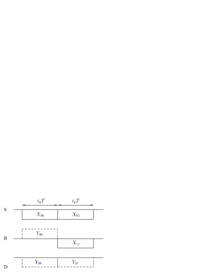
Figure 1: Transmit/Receive signals for source (S), relay (R) and destination (D)

We now consider separately the case when the relay manages to decode the source message and the case when it does not.

$\bullet$ Case when the relay decodes the source message

By referring to (3), we can check that the relay is able to decode the source message if the event

$$\mathcal{E}=\{\omega:t_{0}\log(1+\alpha_{0}\rho G_{01}(\omega))>R\}$$ (4)

is realized. If this is the case, the relay transmits during the remainder of the frame (slot 1) the corresponding codeword of length $t_{1}T$ from its own codebook. The relay codebook is assumed to be independent from the codebook of the source and is composed of $\left\lfloor e^{RT}\right\rfloor$ Gaussian independent vectors with independent $\mathcal{CN}(0,1)$ elements each. We denote by $X_{11}$ the codeword selected by the relay. The latter transmits thus the vector $\sqrt{\alpha_{1}\rho}X_{11}$, where the factor $\alpha_{1}$ is the amplitude gain applied by the relay. This means that $\alpha_{1}\rho T$ is the relay share of the total energy available for the transmission. Finally, during the slots 0 and 1, the destination receives the signal

$$[Y_{20}^{\mathrm{T}},Y_{21}^{\mathrm{T}}]^{\mathrm{T}}={\bf H}_{\mathcal{E}}[X_{00}^{\mathrm{T}},X_{01}^{\mathrm{T}},X_{11}^{\mathrm{T}}]^{\mathrm{T}}+[V_{20}^{\mathrm{T}},V_{21}^{\mathrm{T}}]^{\mathrm{T}}\>,$$ (5)

where

$${\bf H}_{\mathcal{E}}=\left[\begin{array}[]{lll}\sqrt{\alpha_{0}\rho}H_{02}{\bf I}_{t_{0}T}&0&0\\ 0&\sqrt{\alpha_{0}\rho}H_{02}{\bf I}_{t_{1}T}&\sqrt{\alpha_{1}\rho}H_{12}{\bf I}_{t_{1}T}\end{array}\right]\>,$$

and where components of vector $V_{20}$ (resp. $V_{21}$) are unit variance AWGN at the destination during slot 0 (resp. slot 1).

$\bullet$ Case when the relay does not decode the source message

This is the case when the event $\overline{\mathcal{E}}$ is realized. The relay quantizes in this case the received signal during slot 0 and transmits a coded version of the quantized vector towards the destination during slot 1 using the following steps.
a) Quantization: Denote by $\tilde{Y}_{10}$ the quantized version of the received vector $Y_{10}$. Vector $\tilde{Y}_{10}$ is constructed as follows. Clearly, all $t_{0}T$ components of vector $Y_{10}$ are independent and $\mathcal{CN}(0,\alpha_{0}\rho G_{01}+1)$ distributed. Denote by $\Delta^{2}(\rho)$ the desired squared-error distortion per vector component:

$$\mathbb{E}|\tilde{Y}_{10}(i)-Y_{10}(i)|^{2}\leq\Delta^{2}(\rho)\>.$$

It is clear that letting the quantization squared-error depend on the SNR $\rho$ provides us with an additional degree of freedom in the design of the protocol as we will see. The Rate Distortion Theorem for Gaussian sources [27] tells us that there exists a $(\left\lfloor e^{Q(\rho)t_{0}T}\right\rfloor,t_{0}T)$-rate distortion code (for some $Q(\rho)>0$) which is achievable for the distortion $\Delta^{2}(\rho)$ if the following condition is satisfied

$$Q(\rho)>\log\left(\frac{\alpha_{0}\rho G_{01}+1}{\Delta^{2}(\rho)}\right)\>.$$ (6)

In practice, such a code can be constructed by properly selecting the quantized vector $\tilde{Y}_{10}$ among a quantizer-codebook formed by $\left\lfloor e^{Q(\rho)t_{0}T}\right\rfloor$ independent random vectors with distribution $\mathcal{CN}(0,(\alpha_{0}\rho G_{01}+$ $1-\Delta^{2}(\rho))\mathbf{I}_{t_{0}T})$. Vector $\tilde{Y}_{10}$ is selected from this codebook in such a way that sequences $Y_{10}$ and $\tilde{Y}_{10}$ are jointly typical w.r.t. the joint distribution $p_{(Y,\tilde{Y})}$ given by

$$Y=\tilde{Y}+\Delta(\rho)Z\>,$$ (7)

where $\tilde{Y}$ and $Z$ are independent random variables with respective distributions $\mathcal{CN}(0,\alpha_{0}\rho G_{01}+1-$ $\Delta^{2}(\rho))$ and $\mathcal{CN}(0,1)$. Condition (6) ensures that such a vector $\tilde{Y}_{10}$ exists with high probability as $T\to\infty$.

Parameter $Q(\rho)$ can be interpreted as the number of nats used to quantize one component of the received vector $Y_{10}$. This parameter must be chosen such that condition (6) is satisfied. As the rhs of (6) depends on the channel gain $G_{01}$, it looks impossible at first glance to construct a fixed quantizer which is successful for any channel state. Nevertheless, recall that we are considering the case where event $\mathcal{E}$ is not realized i.e., $t_{0}\log(1+\alpha_{0}\rho G_{01})<R$. In order to guarantee that condition (6) always hold, it is thus sufficient to define

$$Q(\rho)=\log\left(\frac{K}{\Delta^{2}(\rho)}\right)\>,$$ (8)

where $K$ is any constant such that $K\geq e^{\frac{R}{t_{0}}}$. We choose $K=e^{\frac{R}{t_{0}}}$. In order to complete the definition of the quantizer, we still need to define the way $\Delta^{2}(\rho)$ depends on the SNR $\rho$. This issue is addressed at the end of the current section.
Remark: Note that condition (6) implies that the following inequality should hold

$$\alpha_{0}\rho G_{01}+1>\Delta^{2}(\rho)\>.$$ (9)

Condition (9) is indeed necessary for the construction of the quantization code because it ensures that the variance $\alpha_{0}\rho G_{01}+1-\Delta^{2}(\rho)$ of each component of the codewords is positive. The quantization step is thus possible provided that the event

$$\mathcal{S}=\left\{\omega:\alpha_{0}\rho G_{01}(\omega)+1>\Delta^{2}(\rho)\right\}.$$ (10)

is realized. In case the complementary event $\overline{\mathcal{S}}$ is realized, the relay does not quantize the source message and remains silent during slot 1. The latter case happens with negligible probability provided that $\Delta^{2}(\rho)$ is chosen properly.
b) Forwarding the Relay Message: During the second slot of length $t_{1}T$, the relay must forward the index of the quantized vector among the possible $\left\lfloor e^{Q(\rho)t_{0}T}\right\rfloor$ ones. To that end, it uses a Gaussian codebook with rate $Q(\rho)t_{0}/t_{1}$. If we denote by $X_{11}$ the corresponding codeword, the signal transmitted by the relay can be written as $\sqrt{\phi(\rho)}X_{11}$, where $\phi(\rho)$ is the power of the relay.

Function $\phi(\rho)$ should be selected such that the power constraint given by (2) is respected. A possible choice would be $\phi(\rho)=\alpha_{1}\rho$, which is the same power that the relay spends when event $\cal E$ is realized. In this case, the relay transmits during slot 1 at the same constant power $\alpha_{1}\rho$ regardless of the fact that the source message has been decoded or not. Of course, the factor $\alpha_{1}$ should be fixed in this case such that constraint (2) is respected. While this choice for $\phi(\rho)$ is relatively simple, other possible choices which may lead to better performance of the DoQF without violating the average power constraint are discussed at the end of the current section.
c) Processing at Destination: In case the relay has quantized the source message (event $\mathcal{S}$ defined by (10) is realized), the destination proceeds as follows. It first tries to recover the relay message $X_{11}$ received during slot 1 and uses it to help decode the source message. The signal of length $t_{1}T$ received by the destination during the second slot can be written as

$$Y_{21}=\sqrt{\phi(\rho)}H_{12}X_{11}+\sqrt{\alpha_{0}\rho}H_{02}X_{01}+V_{21}\>.$$ (11)

Note that (11) can be seen as a Multiple Access Channel (MAC). In order to recover $X_{11}$ (and consequently $\tilde{Y}_{10}$) from (11), the destination interprets the source contribution as noise. It succeeds in recovering $\tilde{Y}_{10}$ in case the event

$$\mathcal{F}=\left\{\omega:t_{1}\log\left(1+\frac{\phi(\rho)G_{12}(\omega)}{\alpha_{0}\rho G_{02}(\omega)+1}\right)>Q(\rho)t_{0}\right\}$$ (12)

is realized. We distinguish between three possible cases.
Events $\mathcal{S}$ and $\boldsymbol{\mathcal{F}}$ are realized: In this case, the contribution of $X_{11}$ in (11) can be canceled, and the resulting signal can be written as $Y_{21}^{{}^{\prime}}=\sqrt{\alpha_{0}\rho}H_{02}X_{01}+V_{21}$. Moreover, it is a straightforward result of (7) that the conditional distribution $p_{\tilde{Y}|Y}$ is Gaussian with mean $\mathbb{E}\left[\tilde{Y}|Y\right]=\frac{1+\alpha_{0}\rho G_{01}-\Delta^{2}(\rho)}{1+\alpha_{0}\rho G_{01}}Y$ and variance $\textrm{var}\left(\tilde{Y}|Y\right)=\frac{\Delta^{2}(\rho)\left(1+\alpha_{0}\rho G_{01}-\Delta^{2}(\rho)\right)}{1+\alpha_{0}\rho G_{01}}$. We thus write

$$\tilde{Y}_{10}=\frac{1+\alpha_{0}\rho G_{01}-\Delta^{2}(\rho)}{1+\alpha_{0}\rho G_{01}}Y_{10}+\sqrt{\frac{\Delta^{2}(\rho)\left(1+\alpha_{0}\rho G_{01}-\Delta^{2}(\rho)\right)}{1+\alpha_{0}\rho G_{01}}}\tilde{Z}\>,$$ (13)

where vector $\tilde{Z}$ is AWGN independent of $Y_{10}$ such that each of its components $\tilde{Z}(i)$ satisfies $\tilde{Z}(i)\sim\mathcal{CN}(0,1)$. Plugging $Y_{10}=\sqrt{\alpha_{0}\rho}H_{01}X_{00}+V_{10}$ into (13), it follows that

$$\tilde{Y}_{10}=\sqrt{\gamma(G_{01},\rho)\alpha_{0}\rho}H_{01}X_{00}+\tilde{V}_{10}\>,$$

where $\gamma(G_{01},\rho)=\frac{\left(1+\alpha_{0}\rho G_{01}-\Delta^{2}(\rho)\right)^{2}}{\left(1+\alpha_{0}\rho G_{01}\right)^{2}}$ and where vector $\tilde{V}_{10}$ is AWGN whose components satisfy $\tilde{V}_{10}(i)\sim\mathcal{CN}\big{(}0,\gamma(G_{01},\rho)+\Delta^{2}(\rho)\sqrt{\gamma(G_{01},\rho)}\big{)}$. In order to decode the source message, the overall received signal can be reconstructed as $Y_{2}=\left[Y_{20}^{\mathrm{T}},\tilde{Y}_{10}^{\mathrm{T}},(Y_{21}^{{}^{\prime}})^{\mathrm{T}}\right]^{\mathrm{T}}$ given by

$$Y_{2}=\mathbf{H}_{\mathcal{F}}[X_{00}^{\mathrm{T}},X_{01}^{\mathrm{T}}]^{\mathrm{T}}+\check{V}_{10},$$ (14)

where

$$\mathbf{H}_{\mathcal{F}}=\left[\begin{array}[]{cc}\sqrt{\alpha_{0}\rho}H_{02}\mathbf{I}_{t_{0}T}&0\\ \sqrt{\gamma(G_{01},\rho)\alpha_{0}\rho}H_{01}\mathbf{I}_{t_{0}T}&0\\ 0&\sqrt{\alpha_{0}\rho}H_{02}\mathbf{I}_{t_{1}T}\end{array}\right]\>,$$

and where $\check{V}_{10}=\left[V_{20}^{T},\tilde{V}_{10}^{T},V_{21}^{T}\right]^{T}$ is an additive Gaussian noise of zero mean and and whose covariance matrix is given by

$$\mathbb{E}[\check{V}_{10}\check{V}_{10}^{*}]=\left[\begin{array}[]{ccc}\mathbf{I}_{t_{0}T}&0&0\\ 0&\sqrt{\gamma(G_{01},\rho)+\Delta^{2}(\rho)\sqrt{\gamma(G_{01},\rho)}}\mathbf{I}_{t_{0}T}&0\\ 0&0&\mathbf{I}_{t_{1}T}\end{array}\right]\>.$$

Events $\mathcal{S}$ and $\boldsymbol{\overline{\mathcal{F}}}$ are realized: The destination will only be able to use $Y_{20}$, the signal received during slot 0, to recover the source message. Notice that in such a case, we get $Y_{20}=\sqrt{\alpha_{0}\rho}H_{02}X_{00}+V_{20}$.

Event $\boldsymbol{\overline{\mathcal{S}}}$ is realized: In this case, condition (9) is not satisfied and the relay does not quantize the source message. This is like the case of a non cooperative transmission.

Finally, the outage probability of the DoQF protocol writes

$$P_{o}(\rho)=P_{o,1}(\rho)+P_{o,2}(\rho)+P_{o,3}(\rho)+P_{o,4}(\rho)\>.$$ (15)

where

• $P_{o,1}(\rho)$ is the probability that the destination is in outage and that the event $\mathcal{E}$ is realized. We thus get

  $$P_{o,1}(\rho)=\mathrm{Pr}[t_{0}\log(1+\alpha_{0}\rho G_{02})+t_{1}\log(1+\alpha_{0}\rho G_{02}+\alpha_{1}\rho G_{12})\leq R](1-\mathrm{Pr}\left[\overline{\mathcal{E}}\right])\>.$$ (16)

  where $\mathrm{Pr}\left[\overline{\mathcal{E}}\right]$ is the probability that the relay does not succeed in decoding the source message;

• $P_{o,2}(\rho)$ is the probability that the destination is in outage and that events $\overline{\mathcal{E}}$, $\mathcal{F}$ and $\mathcal{S}$ are realized. We thus have

  $$P_{o,2}(\rho)=\mathrm{Pr}\Bigg{[} t_{1}\log(1+\alpha_{0}\rho G_{02})+t_{0}\log\left(1+\alpha_{0}\rho G_{02}+\frac{\gamma(G_{01},\rho)\alpha_{0}\rho G_{01}}{\gamma(G_{01},\rho)+\Delta^{2}(\rho)\sqrt{\gamma(G_{01},\rho)}}\right)\leq R,$$

  $$\overline{\mathcal{E}},\mathcal{F},\mathcal{S}\Bigg{]}\>;$$ (17)

• $P_{o,3}(\rho)$ is the probability that the destination is in outage and that events $\overline{\mathcal{E}}$, $\overline{\mathcal{F}}$ and $\mathcal{S}$ are realized. Therefore we have

  $$P_{o,3}(\rho)=\mathrm{Pr}[t_{0}\log(1+\alpha_{0}\rho G_{02})\leq R,\overline{\mathcal{E}},\overline{\mathcal{F}},\mathcal{S}]\>;$$ (18)

• $P_{o,4}(\rho)$ is the probability that the destination is in outage and that events $\overline{\mathcal{E}}$ and $\overline{\mathcal{S}}$ are realized. One can easily check that

  $$P_{o,4}(\rho)=\mathrm{Pr}\Big{[}\log(1+\alpha_{0}\rho G_{02})\leq R,\overline{\mathcal{E}},\overline{\mathcal{S}}\Big{]}\>.$$ (19)

In Figure 2, the data processing steps at the destination node are summarized.

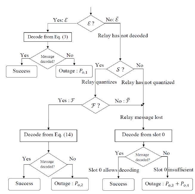
Figure 2: Data processing at the destination

II-B On the selection of parameters $t_{0},t_{1},\alpha_{0},\alpha_{1},\phi(\rho),\Delta^{2}(\rho)$

In order to complete the definition of the DoQF protocol, we still need to provide a method for the selection of the relative slots durations $t_{0}$, $t_{1}$, the amplitude factors $\alpha_{0}$, $\alpha_{1}$, the relay power $\phi(\rho)$ and the quantization squared-error $\Delta^{2}(\rho)$.

We first begin by considering parameters $t_{0}$, $t_{1}$, $\alpha_{0}$, $\alpha_{1}$, and $\phi(\rho)$. It is clear that these parameters should be selected such that the power constraint (2) is respected. Recall that the power constraint (2) is a long term constraint which ensures that the average total energy $E_{0}+E_{1}$ spent by the network does not exceed a certain value i.e., $E_{0}+E_{1}\leq\rho T$. In order to make explicit this power constraint, let us derive the average energy spent by both the source and the relay to transmit a block of $RT$ nats. The source transmits the signal $[\sqrt{\alpha_{0}\rho}X_{00},\sqrt{\alpha_{0}\rho}X_{01}]$ spending the energy $E_{0}=\alpha_{0}\rho T$. If the event $\mathcal{E}$ is realized i.e., if the relay decodes the source message, then the relay transmits the signal $\sqrt{\alpha_{1}\rho}X_{11}$ and spends $\alpha_{1}\rho t_{1}T$ Joules. If the events $\mathcal{\overline{E}}$ and $\mathcal{S}$ are realized, the relay transmits $\sqrt{\phi(\rho)}X_{11}$ spending $\phi(\rho)t_{1}T$ Joules. As for the case where the event $\overline{\mathcal{S}}$ is realized, the relay remains inactive spending no energy. The average energy spent by the relay is thus $E_{1}=\alpha_{1}\rho t_{1}T\left(1-\mathrm{Pr}\left[\overline{\mathcal{E}}\right]\right)+\phi(\rho)t_{1}T\textrm{Pr}\left[\mathcal{\overline{E}},\mathcal{S}\right]$. Putting all pieces together, the power constraint given by (2) can be written as

$$\alpha_{0}\rho+\alpha_{1}\rho t_{1}\left(1-\mathrm{Pr}\left[\overline{\mathcal{E}}\right]\right)+\phi(\rho)t_{1}\textrm{Pr}\left[\mathcal{\overline{E}},\mathcal{S}\right]\leq\rho\>.$$ (20)

Parameters $t_{0}$, $t_{1}$, $\alpha_{0}$, $\alpha_{1}$ and $\phi(\rho)$ should thus be selected such that constraint (20) is respected. This task will be addressed in Section III assuming that the performance metric is the outage gain, and in Section IV assuming that the performance metric is the DMT. Note that since the probability $\textrm{Pr}\left[\mathcal{\overline{E}},\mathcal{S}\right]$ is in general smaller than $1-\mathrm{Pr}\left[\overline{\mathcal{E}}\right]$ for sufficiently large values of the SNR $\rho$, the power $\phi(\rho)$ can be boosted beyond the value $\alpha_{1}\rho$ without violating the average power constraint given by (20).

Consider now the quantization squared-error distortion $\Delta^{2}(\rho)$, and let us discuss some possible choices for the way $\Delta^{2}(\rho)$ depends on the SNR $\rho$. One possible case is to choose $\Delta^{2}(\rho)$ such that $\lim_{\rho\to\infty}\Delta^{2}(\rho)=0$ i.e., fine quantization is achieved at high SNR. This choice will be revealed relevant when the performance metric is the outage gain (see Section III). As for the case where the performance metric is the DMT, we will see in Section IV that choosing $\lim_{\rho\to\infty}\Delta^{2}(\rho)=0$ is relevant for some values of the multiplexing gain $r$, while it is not for other values.

Now that a detailed description of the DoQF has been provided, the rest of the paper is devoted to the study of the performance of this protocol using two performance metrics: The outage gain and the DMT.

III Outage Probability Analysis of the DoQF Protocol

This section is devoted to the outage gain derivation and its minimization over power and time slot allocation for the DoQF protocol.

III-A Notations and Channel Assumptions

Recall that $H_{ij}$ is the random variable that represents the wireless channel between nodes $i$ and $j$ of the network ($i,j\in\{0,1,2\}$), and that $G_{ij}=|H_{ij}|^{2}$ designates the power gain of this channel. In this section, all variables $G_{ij}$ are assumed to have densities $f_{G_{ij}}(x)$ which are right continuous at zero. This assumption is satisfied in particular by the so-called Rayleigh and Rice channels. Note that except for this mild assumption, we do not make any assumption on the channels probability distributions. We denote by $c_{ij}$ the limit $c_{ij}=f_{G_{ij}}(0^{+})$ and we assume that all these limits are positive. For instance, in the Rayleigh case, $H_{ij}$ is complex circular Gaussian with zero mean and variance $\sigma_{ij}^{2}$. In this case, $G_{ij}$ has the exponential distribution $f_{G_{ij}}(x)=\sigma_{ij}^{-2}\exp(-x/\sigma_{ij}^{2})\mathbf{1}\{x\geq 0\}$, and in particular $c_{ij}=\sigma_{ij}^{-2}$. Here, for any subset $\mathcal{A}$ of $\mathbb{R}$, we denote by $\mathbf{1}\{\mathcal{A}\}$ the indicator function of the set $\mathcal{A}$. More generally, in the Rician case $H_{ij}\sim\mathcal{CN}(m_{ij},\sigma_{ij}^{2})$ where the mean $m_{ij}$ is not necessarily zero, the density is given by

$$f_{G_{ij}}(x)=\frac{1}{\sigma_{ij}^{2}}\exp\left(-\frac{|m_{ij}|^{2}+x}{\sigma_{ij}^{2}}\right)I_{0}\left(2\sqrt{x}\frac{|m_{ij}|}{\sigma_{ij}^{2}}\right)\mathbf{1}\{x\geq 0\}\>,$$

where $I_{0}$ is the modified zero order Bessel function of the first kind. As $I_{0}(0^{+})=1$, we have in this case

$$c_{ij}=\frac{1}{\sigma_{ij}^{2}}\exp\left(-\frac{|m_{ij}|^{2}}{\sigma_{ij}^{2}}\right)\>.$$

In this section, the constants $c_{01},c_{02}$ and $c_{12}$ are assumed to be available to the resource allocation unit.

III-B Lower Bound on the Outage Gain of Static Half-Duplex Protocols

Before deriving the outage gain of the proposed DoQF protocol, we first derive a bound on the outage performance of the wide class of half-duplex static relaying protocols. This class is indexed in the following by parameters $t_{0}$, $\alpha_{0}$, $\alpha_{1}$. For each value of these parameters, the class is denoted by ${\cal P}_{\textrm{HD}}(t_{0},\alpha_{0},\alpha_{1})$ and is defined as the set of all half-duplex static relaying protocols which satisfy the following.

• The source has at its disposal a dictionary of $\left\lfloor e^{RT}\right\rfloor$ codewords. Each codeword $X_{0}=\left[X_{00}^{\mathrm{T}},X_{01}^{\mathrm{T}}\right]^{\mathrm{T}}$ is a vector of length $T$ channel uses.

• The source average transmit power $\frac{1}{T}\sum_{i=1}^{T}E\left[|X_{0}(i)|^{2}\right]$ satisfies the following high SNR constraint

  $$\lim_{\rho\to\infty}\frac{\frac{1}{T}\sum_{i=1}^{T}\mathbb{E}\left[|X_{0}(i)|^{2}\right]}{\rho}\leq\alpha_{0}\>.$$ (21)

• The relay listens to the source signal during the first $t_{0}T$ channel uses out of the $T$ channel uses which is the duration of the whole transmission. The relay has at its disposal a dictionary of codewords $X_{11}$ of length $(1-t_{0})T$ channel uses each.

• During the last $(1-t_{0})T$ channel uses of the transmission, the relay average transmit power satisfies

  $$\lim_{\rho\to\infty}\frac{\frac{1}{(1-t_{0})T}\sum_{i=1}^{(1-t_{0})T}\mathbb{E}\left[|X_{11}(i)|^{2}\right]}{\rho}\leq\alpha_{1}\>.$$ (22)

Note that the above definition does not assume any particular distribution of the codewords that compose the codebooks of the source and the relay. Moreover, the definition of the class ${\cal P}_{\textrm{HD}}(t_{0},\alpha_{0},\alpha_{1})$ imposes no constraints on the powers transmitted by the nodes for finite values of the SNR $\rho$. Instead, constraints (21) and (22) restrict only the way the average transmit powers of the source and the relay behave in the high SNR regime.

Theorem 1.

For any static half-duplex relaying protocol from the class ${\cal P}_{\textrm{HD}}(t_{0},\alpha_{0},\alpha_{1})$, the outage gain $\xi=\lim_{\rho\to\infty}\rho^{2}P_{o}(\rho)$ is lower-bounded by $\xi_{\textrm{CS-HD}}$, where

$$\xi_{\mathrm{CS-HD}}= \frac{c_{02}c_{01}}{\alpha_{0}^{2}}\left(\frac{1}{2}+\frac{\exp(2R)}{4t_{0}-2}-\frac{t_{0}\exp(R/t_{0})}{2t_{0}-1}\right)+$$

$$\frac{c_{02}c_{12}}{\alpha_{0}\alpha_{1}}\left(\frac{1}{2}+\frac{\exp(2R)}{4t_{1}-2}-\frac{t_{1}\exp(R/t_{1})}{2t_{1}-1}\right)\>.$$ (23)

The proof of Theorem 1 is provided in Appendix A. The above lower-bound has been derived using the Cut-Set (CS) bound for Half-Duplex (HD) relay channels, as we will see in Appendix A. This explains the use of notation $\xi_{\textrm{CS-HD}}$ with the subscript (CS-HD) to designate this bound.

We now derive and compare the outage gain of the proposed DoQF protocol with the above lower-bound.

III-C Outage Gain of the DoQF Protocol

The following theorem characterizes the outage performance of the proposed protocol at high SNR.

Theorem 2.

Assume that the quantization squared-error distortion $\Delta^{2}(\rho)$ and the relay power $\phi(\rho)$ are chosen such that

$$\lim_{\rho}\phi(\rho)=+\infty,$$ (24)

$$\lim_{\rho}\frac{\phi(\rho)}{\rho^{2}}=0,$$ (25)

$$\lim_{\rho}\Delta^{2}(\rho)=0,$$ (26)

$$\lim_{\rho}\left(\phi(\rho)^{t_{1}}\>\Delta^{2}(\rho)^{t_{0}}\right)=+\infty.$$ (27)

In particular, constraint (25) ensures that the DoQF belongs to the class ${\cal P}_{\textrm{HD}}(t_{0},\alpha_{0},\alpha_{1})$. The outage gain $\xi_{\textrm{DoQF}}$ associated with the proposed DoQF protocol coincides with the lower-bound given by (23):

$$\xi_{\mathrm{DoQF}}=\xi_{\mathrm{CS-HD}}\>.$$

The proof of Theorem 2 is given in Subsection III-D. Theorem 2 states that the DoQF protocol is outage-gain-optimal in the wide class of half-duplex static relaying protocols.

As a matter of fact, the outage gain associated with the DoQF protocol depends on both the quantization error $\Delta^{2}(\rho)$ and the power $\phi(\rho)$ allocated to the relay during slot 1. Theorem 2 states that it is sufficient to choose $\Delta^{2}(\rho)$ and $\phi(\rho)$ such that constraints (24)-(27) are satisfied in order for the outage gain of the DoQF to be equal to the lower-bound $\xi_{\textrm{CS-HD}}$. The choice $\phi(\rho)=\alpha_{1}\rho$ is for instance a possible candidate for $\phi(\rho)$, provided that $\Delta^{2}(\rho)$ is chosen such that (26) and (27) are satisfied i.e., such that $\rho^{-\frac{t_{1}}{t_{0}}}\stackrel{{\scriptstyle.}}{{<}}\Delta^{2}(\rho)\stackrel{{\scriptstyle.}}{{<}}1$. It is therefore optimal from an outage gain perspective to let the relay transmit at a constant power regardless of whether the source message has been decoded with success or not.

III-D Proof of Theorem 2

Recall the definition of $P_{o}(\rho)$ given by (15) as the outage probability associated with the DoQF protocol. In order to prove Theorem 2, we need to show that $\rho^{2}P_{o}(\rho)$ converges as $\rho\to\infty$ and to derive the outage gain $\xi_{\textrm{DoQF}}$ given by $\xi_{\textrm{DoQF}}=\lim_{\rho\to\infty}\rho^{2}P_{o}(\rho)$. According to (15), $P_{o}(\rho)=P_{o,1}(\rho)+P_{o,2}(\rho)+P_{o,3}(\rho)+P_{o,4}(\rho)$, where $P_{o,1}(\rho)$, $P_{o,2}(\rho)$, $P_{o,3}(\rho)$ and $P_{o,4}(\rho)$ are defined by (16), (17), (18) and (19) respectively. Therefore, we need to first compute the limits $\lim_{\rho\to\infty}\rho^{2}P_{o,1}(\rho)$, $\lim_{\rho\to\infty}\rho^{2}P_{o,2}(\rho)$, $\lim_{\rho\to\infty}\rho^{2}P_{o,3}(\rho)$ and $\lim_{\rho\to\infty}\rho^{2}P_{o,4}(\rho)$ in order to obtain the outage gain $\xi_{\textrm{DoQF}}$. It has been proved in [26] that

$$\lim_{\rho\to\infty}\rho^{2}P_{o,1}(\rho)=\frac{c_{02}c_{12}}{\alpha_{0}\alpha_{1}}\int_{\mathbb{R}_{+}^{2}}\mathbf{1}\{t_{0}\log(1+u)+t_{1}\log(1+u+v)\leq R\}dudv\>,$$ (28)

where $c_{01}$ and $c_{12}$ has been defined in Subsection III-A as $c_{01}=f_{G_{01}}(0+)$ and $c_{12}=f_{G_{12}}(0+)$ respectively. The steps of the proof that (28) holds are very similar to the steps given below for the derivation of $\lim_{\rho\to\infty}\rho^{2}P_{o,2}(\rho)$. Refer to the definition of $P_{o,2}(\rho)$ given by (17) as

$$P_{o,2}(\rho)=\mathrm{Pr}\Bigg{[} t_{1}\log(1+\alpha_{0}\rho G_{02})+t_{0}\log\left(1+\alpha_{0}\rho G_{02}+\frac{\gamma(G_{01},\rho)\alpha_{0}\rho G_{01}}{\gamma(G_{01},\rho)+\Delta^{2}(\rho)\sqrt{\gamma(G_{01},\rho)}}\right)<R,$$

$$\overline{\mathcal{E}},\mathcal{F},\mathcal{S}\Bigg{]}\>,$$ (29)

where $\gamma(G_{01},\rho)=\frac{\left(1+\alpha_{0}\rho G_{01}-\Delta^{2}(\rho)\right)^{2}}{\left(1+\alpha_{0}\rho G_{01}\right)^{2}}$. Plugging the definitions of events $\mathcal{E}$, $\mathcal{S}$ and $\mathcal{F}$ given respectively by (4), (10) and (12) into (29) leads to

$$P_{o,2}(\rho)= \int_{\mathbb{R}_{+}^{3}}\mathbf{1}\left\{t_{1}\log(1+\alpha_{0}\rho x)+t_{0}\log\left(1+\alpha_{0}\rho x+\frac{\gamma(y,\rho)\alpha_{0}\rho y}{\gamma(y,\rho)+\Delta^{2}(\rho)\sqrt{\gamma(y,\rho)}}\right)\leq R\right\}$$

$$\times\mathbf{1}\left\{t_{0}\log(1+\alpha_{0}\rho y)\leq R\right\}\mathbf{1}\left\{1+\alpha_{0}\rho y>\Delta^{2}(\rho)\right\}$$

$$\times\mathbf{1}\left\{t_{1}\log\left(1+\frac{\phi(\rho)z}{1+\alpha_{0}\rho x}\right)>t_{0}Q(\rho)\right\}f_{G_{02}}(x)f_{G_{01}}(y)f_{G_{12}}(z)dxdydz\>,$$

By making the change of variables $u=\alpha_{0}\rho x$ and $v=\alpha_{0}\rho y$ we obtain

$$\rho^{2}P_{o,2}(\rho)=\frac{1}{\alpha_{0}^{2}} \int_{\mathbb{R}_{+}^{3}}\mathbf{1}\left\{t_{1}\log(1+u)+t_{0}\log\left(1+u+\frac{\gamma(v,\rho)v}{\gamma(v,\rho)+\Delta^{2}(\rho)\sqrt{\gamma(v,\rho)}}\right)\leq R\right\}$$

$$\times\mathbf{1}\left\{t_{0}\log(1+v)\leq R\right\}\mathbf{1}\left\{1+v>\Delta^{2}(\rho)\right\}$$

$$\times\mathbf{1}\left\{t_{1}\log\left(1+\frac{\phi(\rho)z}{1+u}\right)>t_{0}Q(\rho)\right\}f_{G_{02}}\left(\frac{u}{\alpha_{0}\rho}\right)f_{G_{01}}\left(\frac{v}{\alpha_{0}\rho}\right)f_{G_{12}}(z)dudvdz\>.$$ (30)

Since $Q(\rho)=\log\left(K/\Delta^{2}(\rho)\right)$ as given by (8), it is possible and useful to write the last indicator as follows.

$$\mathbf{1}\left\{t_{1}\log\left(1+\frac{\phi(\rho)z}{1+u}\right)>t_{0}Q(\rho)\right\}=\mathbf{1}\left\{z>(1+u)\theta(\rho)\right\}\>,$$ (31)

where

$$\theta(\rho)=\frac{K^{\frac{t_{0}}{t_{1}}}}{\phi(\rho)\left(\Delta^{2}(\rho)\right)^{\frac{t_{0}}{t_{1}}}}-\frac{1}{\phi(\rho)}\>.$$ (32)

Define the function $\Phi(u,v,z,\rho)$ as the integrand in the rhs of (30) and let $\mathcal{C}$ be the compact subset of $\mathbb{R}_{+}^{2}$ defined as $\mathcal{C}=\Bigg{\{}(u,v)\in\mathbb{R}_{+}^{2},t_{1}\log(1+u)+t_{0}\log\left(1+u+\frac{\gamma(v,\rho)v}{\gamma(v,\rho)+\Delta^{2}(\rho)\sqrt{\gamma(v,\rho)}}\right)\leq R,t_{0}\log(1+v)\leq$ $R\Bigg{\}}$. As $f_{G_{02}}$ and $f_{G_{01}}$ are right continuous at zero, then the function $(u,v)\mapsto f_{G_{02}}\left(\frac{u}{\alpha_{0}\rho}\right)f_{G_{01}}\left(\frac{v}{\alpha_{0}\rho}\right)$ is bounded on $\mathcal{C}$ for $\rho$ large enough i.e., there exist $\rho_{0}>0$ and $M>0$ such that $\forall\rho\geq\rho_{0}$, $f_{G_{02}}\left(\frac{u}{\alpha_{0}\rho}\right)f_{G_{01}}\left(\frac{v}{\alpha_{0}\rho}\right)\leq M$. It is straightforward to verify that the following inequalities hold for all $\rho\geq\rho_{0}$:

$$\Phi(u,v,z,\rho)\leq M\times\mathbf{1}\left\{t_{1}\log(1+u)+t_{0}\log\left(1+u+\frac{\gamma(v,\rho)v}{\gamma(v,\rho)+\Delta^{2}(\rho)\sqrt{\gamma(v,\rho)}}\right)\leq R\right\}$$

$$\times\mathbf{1}\left\{t_{0}\log(1+v)\leq R\right\}\mathbf{1}\left\{1+v>\Delta^{2}(\rho)\right\}$$

$$\times\mathbf{1}\left\{z>(1+u)\theta(\rho)\right\}f_{G_{12}}(z)$$

$$\leq M\times\mathbf{1}\left\{\log(1+u)\leq R\right\}\times\mathbf{1}\left\{t_{0}\log(1+v)\leq R\right\}f_{G_{12}}(z)\>.$$

The rhs of the latter inequality is an integrable function on $\mathbb{R}_{+}^{3}$ and it does not depend on $\rho$. Therefore, we can apply Lebesgue’s Dominated Convergence Theorem (DCT) in order to compute $\lim_{\rho\to\infty}\rho^{2}P_{o,2}(\rho)$ in (30). Note first that $\lim_{\rho\to\infty}\Delta^{2}(\rho)=0$, $\lim_{\rho\to\infty}\frac{\gamma(v,\rho)}{\gamma(v,\rho)+\Delta^{2}(\rho)\sqrt{\gamma(v,\rho)}}=1$ and $\lim_{\rho\to\infty}\theta(\rho)=0$ due to assumptions (24)- (27). After some algebra, we can easily show that the following result holds.

$$\lim_{\rho\to\infty}\rho^{2}P_{o,2}(\rho)=\frac{c_{02}c_{01}}{\alpha_{0}^{2}}\int_{\mathbb{R}_{+}^{2}}\mathbf{1}\left\{t_{1}\log(1+u)+t_{0}\log\left(1+u+v\right)\leq R\right\}dudv\>.$$ (33)

We now prove that $\lim_{\rho\to\infty}\rho^{2}P_{o,3}(\rho)=0$. First, recall that $P_{o,3}(\rho)=\mathrm{Pr}[t_{0}\log(1+\alpha_{0}\rho G_{02})<R,\overline{\mathcal{E}},\overline{\mathcal{F}},\mathcal{S}]$. Plugging the definition of events $\mathcal{E}$, $\mathcal{S}$ and $\mathcal{F}$ from (4), (10) and (12) respectively into the latter equation leads to

$$P_{o,3}(\rho)= \int_{\mathbb{R}_{+}^{3}}\mathbf{1}\left\{t_{0}\log(1+\alpha_{0}\rho x)\leq R\right\}\mathbf{1}\left\{t_{0}\log(1+\alpha_{0}\rho y)\leq R\right\}\mathbf{1}\left\{1+\alpha_{0}\rho y>\Delta^{2}(\rho)\right\}$$

$$\times\mathbf{1}\left\{t_{1}\log\left(1+\frac{\phi(\rho)z}{1+\alpha_{0}\rho x}\right)\leq t_{0}Q(\rho)\right\}f_{G_{02}}(x)f_{G_{01}}(y)f_{G_{12}}(z)dxdydz\>,$$

Defineing $u=\alpha_{0}\rho x$ and $v=\alpha_{0}\rho y$, we get

$$P_{o,3}(\rho)=\frac{1}{\alpha_{0}^{2}\rho^{2}} \int_{\mathbb{R}_{+}^{3}}\mathbf{1}\left\{t_{0}\log(1+u)\leq R\right\}\mathbf{1}\left\{t_{0}\log(1+v)\leq R\right\}\mathbf{1}\left\{1+v>\Delta^{2}(\rho)\right\}$$

$$\times\mathbf{1}\left\{t_{1}\log\left(1+\frac{\phi(\rho)z}{1+u}\right)\leq t_{0}Q(\rho)\right\}f_{G_{02}}\left(\frac{u}{\alpha_{0}\rho}\right)f_{G_{01}}\left(\frac{v}{\alpha_{0}\rho}\right)f_{G_{12}}(z)dudvdz\>.$$

As we did in (31), we write the last indicator as follows.

$$\mathbf{1}\left\{t_{1}\log\left(1+\frac{\phi(\rho)z}{1+u}\right)\leq t_{0}Q(\rho)\right\}=\mathbf{1}\left\{z\leq(1+u)\theta(\rho)\right\}\>,$$

where $\theta(\rho)$ is defined by (32). In analogy with the approach we used to compute $\lim_{\rho\to\infty}\rho^{2}P_{o,2}(\rho)$, we define $\mathcal{C}_{1}$ as the compact subset of $\mathbb{R}_{+}^{3}$ satisfying $\mathcal{C}_{1}=\big{\{}(u,v,z)\in\mathbb{R}_{+}^{3}$, $t_{0}\log(1+u)\leq R$, $t_{0}\log(1+v)\leq R$, $z\leq(1+u)\theta(\rho)\big{\}}$. Next, we use the fact that $f_{G_{02}}$, $f_{G_{01}}$ and $f_{G_{12}}$ are right continuous at zero, along with $\lim_{\rho\to\infty}\theta(\rho)=0$, to show that the function $(u,v,z)\mapsto f_{G_{02}}\left(\frac{u}{\alpha_{0}\rho}\right)f_{G_{01}}\left(\frac{v}{\alpha_{0}\rho}\right)f_{G_{12}}(z)$ is bounded on $\mathcal{C}_{1}$ for $\rho$ large enough i.e., there exist $\rho_{1}>0$ and $M_{1}>0$ such that $\forall\rho\geq\rho_{1}$, $f_{G_{02}}\left(\frac{u}{\alpha_{0}\rho}\right)f_{G_{01}}\left(\frac{v}{\alpha_{0}\rho}\right)f_{G_{12}}(z)\leq M_{1}$. It follows that the following inequalities hold for all $\rho\geq\rho_{1}$:

$$\rho^{2}P_{o,3}(\rho) \leq\frac{M_{1}}{\alpha_{0}^{2}}\int_{\mathbb{R}_{+}^{2}}\mathbf{1}\left\{1+u\leq e^{\frac{R}{t_{0}}}\right\}\mathbf{1}\left\{z\leq(1+u)\theta(\rho)\right\}dudz$$

$$\leq\frac{M_{1}}{\alpha_{0}^{2}}\int_{\mathbb{R}_{+}}\mathbf{1}\left\{z\leq e^{\frac{R}{t_{0}}}\theta(\rho)\right\}dz\leq\frac{M_{1}}{\alpha_{0}^{2}}\int_{0}^{e^{\frac{R}{t_{0}}}\theta(\rho)}dz=\frac{M_{1}}{\alpha_{0}^{2}}e^{\frac{R}{t_{0}}}\theta(\rho)\>.$$

Now since $\lim_{\rho\to\infty}\theta(\rho)=0$ due to assumptions (24)-(27), it follows that $\lim_{\rho\to\infty}\rho^{2}P_{o,3}(\rho)=0$. We can prove in the same way and without difficulty that $\lim_{\rho\to\infty}\rho^{2}P_{o,4}(\rho)=0$.

Putting all pieces together,

$$\lim_{\rho\to\infty}\rho^{2}P_{o}= \lim_{\rho\to\infty}\rho^{2}P_{o,1}(\rho)+\lim_{\rho\to\infty}\rho^{2}P_{o,2}(\rho)+\lim_{\rho\to\infty}\rho^{2}P_{o,3}(\rho)+\lim_{\rho\to\infty}\rho^{2}P_{o,4}(\rho)$$

$$= \frac{c_{02}c_{12}}{\alpha_{0}\alpha_{1}}\int_{\mathbb{R}_{+}^{2}}\mathbf{1}\{t_{0}\log(1+u)+t_{1}\log(1+u+v)\leq R\}dudv$$

$$+ \frac{c_{02}c_{01}}{\alpha_{0}^{2}}\int_{\mathbb{R}_{+}^{2}}\mathbf{1}\left\{t_{1}\log(1+u)+t_{0}\log\left(1+u+v\right)\leq R\right\}dudv\>.$$ (34)

The remaining task is to prove that the rhs of (III-D) is equal to the rhs of (23). This can be done by making the change of variables $x=\log(1+u)$ and $y=\log\left(1+\frac{v}{1+u}\right)$ in (III-D). The details of the proof can be found in [26]. The proof of Theorem 2 is thus complete.

III-E Power and Time Optimization

Our aim in this subsection is to derive the slots relative durations $t_{0}$, $t_{1}$ and the power allocation parameters $\alpha_{0}$, $\alpha_{1}$ that minimizes the outage gain $\xi_{\textrm{DoQF}}$ associated with the DoQF protocol. This minimization should be done subject to the power constraint given by (20). Let us examine the above constraint when the SNR $\rho$ tends to infinity. We first divide the two sides of the power constraint by $\rho$, which leads to $\alpha_{0}+\alpha_{1}t_{1}\left(1-\mathrm{Pr}\left[\overline{\mathcal{E}}\right]\right)+\frac{\phi(\rho)}{\rho}t_{1}\textrm{Pr}\left[\mathcal{\overline{E}},\mathcal{S}\right]\leq 1$, where $\mathrm{Pr}[\overline{\mathcal{E}}]=\mathrm{Pr}\left[t_{0}\log(1+\alpha_{0}\rho G_{01})\leq R\right]$. It is useful to write the term $\frac{\phi(\rho)}{\rho}t_{1}\textrm{Pr}\left[\mathcal{\overline{E}},\mathcal{S}\right]$ in the lhs of the above inequality as $t_{1}\frac{\phi(\rho)}{\rho^{2}}\rho\textrm{Pr}\left[\mathcal{\overline{E}},\mathcal{S}\right]$. Recall that due to (25), $\phi(\rho)$ is chosen such that $\lim_{\rho\to\infty}\frac{\phi(\rho)}{\rho^{2}}=0$. Furthermore, it is straightforward to check that $\rho\textrm{Pr}\left[\mathcal{\overline{E}},\mathcal{S}\right]$ is upper-bounded for any $\rho\in\mathbb{R}_{+}$. Indeed, $\lim_{\rho\to\infty}\rho\textrm{Pr}\left[\mathcal{\overline{E}},\mathcal{S}\right]$ is a constant. Putting all pieces together, the power constraint at high SNR writes as $\alpha_{0}+t_{1}\alpha_{1}\leq 1\>.$ Note that this constraint is not convex in $\alpha_{0},\alpha_{1},t_{1}$ because the function $(\alpha_{1},t_{1})\mapsto\alpha_{1}t_{1}$ is not. It will be convenient to replace it with a convex constraint by making the change of variables $\beta_{0}=\alpha_{0}$ and $\beta_{1}=\alpha_{1}t_{1}$. With these new variables, the power constraint becomes

$$\beta_{0}+\beta_{1}\leq 1\>,$$ (35)

and the outage gain $\xi_{\textrm{DoQF}}$ given by (15) writes

$$\xi_{\textrm{DoQF}}(t_{1},\beta_{0},\beta_{1})= \frac{c_{02}c_{01}}{\beta_{0}^{2}}\left(\frac{1}{2}+\frac{\exp(2R)}{2-4t_{1}}-\frac{(1-t_{1})}{1-2t_{1}}\exp\left(\frac{R}{1-t_{1}}\right)\right)+$$

$$\frac{c_{02}c_{12}t_{1}}{\beta_{0}\beta_{1}}\left(\frac{1}{2}+\frac{\exp(2R)}{4t_{1}-2}-\frac{t_{1}}{2t_{1}-1}\exp\left(\frac{R}{t_{1}}\right)\right)\>.$$ (36)

Using the same arguments of [26], it can be shown that the function $\xi_{\textrm{DoQF}}(t_{1},\beta_{0},\beta_{1})$ is convex on the domain $(0,1)\times(0,\infty)^{2}$. The outage probability minimization at high SNR reduces thus to minimizing $\xi_{\textrm{DoQF}}(t_{1},\beta_{0},\beta_{1})$ given the constraint (35). This in turn reduces to minimizing $\xi_{\textrm{DoQF}}$ on the line segment of $\mathbb{R}_{+}^{2}$ defined by $\beta_{0}+\beta_{1}=1$ i.e., the constraint (35) is met with equality. The function $\xi_{\textrm{DoQF}}(t_{1},\beta_{0},1-\beta_{0})$ defined on the open square $(0,1)^{2}$ is convex as it coincides with the restriction of $\xi_{\textrm{DoQF}}(t_{1},\beta_{0},\beta_{1})$ to a line segment. Furthermore, it is clear that $\xi_{\textrm{DoQF}}(t_{1},\beta_{0},1-\beta_{0})$ goes to infinity on the frontier of $(0,1)^{2}$. Therefore, the minimum is in the interior of $(0,1)^{2}$, and can be obtained easily, for instance by a suitable descent method [28].

IV DMT Analysis of the DoQF Protocol

This section is devoted to the derivation of the DMT of the proposed DoQF protocol.

IV-A Channel Assumptions

In this section, the wireless channels between the different nodes of the network are assumed to be Rayleigh distributed. This assumption is to be compared with the mild assumptions involved in the derivation of the outage gain in Section III, and which apply to a large class of channel distributions, including Rayleigh and Rice channels. Finally, the transmission rate is assumed to be a function of the SNR $\rho$ and to satisfy $R=R(\rho)\stackrel{{\scriptstyle.}}{{=}}r\log\rho$, in accordance with (1).

Before proceeding with the derivation of the DMT of the proposed DoQF protocol, we should first select the way the quantization squared-error $\Delta^{2}(\rho)$ and the relay power $\phi(\rho)$ depend on the SNR $\rho$.

IV-B On the Selection of $\Delta^{2}(\rho)$ and $\phi(\rho)$ from a DMT Perspective

The outage probability $P_{o}$ associated with the DoQF protocol and defined by (15) depends on the quantization squared-error distortion $\Delta^{2}(\rho)$ and on the power $\phi(\rho)$ allocated to the relay during slot 1. Consequently, the DMT associated with the DoQF depends likewise on these two parameters. In Section III, parameters $\Delta^{2}(\rho)$ and $\phi(\rho)$ were chosen such that constraints (24)-(27) are satisfied. Moreover, it was shown that this choice is optimal from an outage gain perspective. In the current section, we are interested in choices of $\Delta^{2}(\rho)$ and $\phi(\rho)$ that are relevant from a DMT perspective. In the sequel, we compute the DMT of the DoQF assuming that

$$\Delta^{2}(\rho)\stackrel{{\scriptstyle.}}{{=}}\rho^{\delta}\>,$$ (37)

where parameter $\delta$ will be fixed later.

As for the power $\phi(\rho)$, it should be chosen such that the best possible DMT is achieved by the protocol without violating the power constraint given by (20). Since we are evaluating the performance of the DoQF protocol from a DMT perspective, this power constraint should be examined in the asymptotic regime where $\rho$ tends to infinity. We remind that the term $\textrm{Pr}\left[\mathcal{\overline{E}},\mathcal{S}\right]$ in (20), to begin with, denotes the probability that events $\overline{\mathcal{E}}$ and $\mathcal{S}$ are realized i.e., $\textrm{Pr}\left[\mathcal{\overline{E}},\mathcal{S}\right]=\mathrm{Pr}\left[t_{0}\log(1+\alpha_{0}\rho G_{01})\leq R(\rho),1+\alpha_{0}\rho G_{01}>\Delta^{2}(\rho)\right]$. It is straightforward to show that $\textrm{Pr}\left[\mathcal{\overline{E}},\mathcal{S}\right]\stackrel{{\scriptstyle.}}{{=}}\rho^{-\left(1-r/t_{0}\right)^{+}}$ provided that $\delta\leq 1-\left(1-\frac{r}{t_{0}}\right)^{+}$. We will see later on that $\delta\leq 1-\left(1-\frac{r}{t_{0}}\right)^{+}$ is the relevant choice for $\delta$ from a DMT point of view, and is thus assumed in the sequel. Plugging this result into (20), the power constraint can be written in the asymptotic regime as

$$\phi(\rho)\stackrel{{\scriptstyle.}}{{\leq}}\rho^{1+\left(1-r/t_{0}\right)^{+}}\>.$$ (38)

In order for the DoQF protocol to achieve the best possible DMT, we should choose $\phi(\rho)$ such that constraint (38) is met with equality. From now on, $\phi(\rho)$ is thus assumed to satisfy $\phi(\rho)\stackrel{{\scriptstyle.}}{{=}}\rho^{1+\left(1-r/t_{0}\right)^{+}}$.

Note that if we choose $\delta$ such that $\delta<0$, then $\Delta^{2}(\rho)$ and $\phi(\rho)$ as given by (37) and (38) also satisfy constraints (24)-(27). However, choosing $\Delta^{2}(\rho)$ and $\phi(\rho)$ that satisfy at the same time constraints  (37)-(38) and constraints (24)-(27) does not necessarily yield the best DMT performance of the protocol, as we will see.

IV-C DMT of the DoQF protocol

Now that the power $\phi(\rho)$ allocated to the relay during slot 1 has been determined, the outage probability of the DoQF protocol depends only on parameters $t_{0}$ and $\delta$. Therefore, the DMT associated with the DoQF protocol should be defined first for fixed values of $t_{0}$ and $\delta$. We denote by $d(t_{0},\delta,r)$ this DMT which is given by

$$d(t_{0},\delta,r)=-\lim_{\rho\to\infty}\frac{\log P_{o}(\rho)}{\log\rho}\>,$$ (39)

where $P_{o}(\rho)$ is the outage probability associated with the protocol. We define the final DMT of DoQF as

$$d_{\mathrm{{DoQF}}}^{*}(r)=\sup_{t_{0},\delta}d(t_{0},\delta,r)\>,$$ (40)

where the maximization is done with respect to parameters $t_{0}$ and $\delta$. Define $t_{0,{\mathrm{DoQF}}}^{*}(r)$ and $\delta_{\mathrm{DoQF}}^{*}(r)$ as the argument of the supremum in (40). Theorem 3 provides the closed-form expression of the final DMT of the DoQF.

Theorem 3.

Assume that the quantization squared-error distortion chosen by the relay satisfies $\Delta^{2}(\rho)\stackrel{{\scriptstyle.}}{{=}}\rho^{\delta}$. The DMT $d_{\mathrm{DoQF}}^{*}(r)$ associated with the DoQF protocol is given by

$$d_{\mathrm{DoQF}}^{*}(r)=\left\{\begin{array}[]{ll}2(1-r)^{+}&\mathrm{for}\>r\leq\frac{1}{4}\\ 2-\frac{r}{1-v^{*}(r)}&\mathrm{for}\>\frac{1}{4}<r\leq\frac{2(\sqrt{5}-1)}{9-\sqrt{5}}\\ 2-\frac{2}{3-\sqrt{5}}r&\mathrm{for}\>\frac{2(\sqrt{5}-1)}{9-\sqrt{5}}<r\leq\frac{\sqrt{5}-1}{\sqrt{5}+1}\\ (2-r)(1-r)&\mathrm{for}\>r>\frac{\sqrt{5}-1}{\sqrt{5}+1}\end{array}\right.\>,$$ (41)

where $v^{*}(r)$ is the unique solution in $\left[\frac{1}{2},\frac{2}{\sqrt{5}+1}\right]$ to the following equation.

$$2(1+r)v^{3}-(4+5r)v^{2}+2(1+4r)v-4r=0\>.$$ (42)

Moreover, the optimal value of $t_{0}$ as function of $r$ that allows to achieve the DMT $d_{\mathrm{DoQF}}^{*}(r)$ is given by

$$t_{0,{\mathrm{DoQF}}}^{*}(r)=\left\{\begin{array}[]{ll}\frac{1}{2}&\mathrm{for}\>0\leq r\leq\frac{1}{4}\\ v^{*}(r)&\mathrm{for}\>\frac{1}{4}<r\leq\frac{2(\sqrt{5}-1)}{9-\sqrt{5}}\\ \frac{2}{\sqrt{5}+1}&\mathrm{for}\>\frac{2(\sqrt{5}-1)}{9-\sqrt{5}}<r\leq\frac{\sqrt{5}-1}{\sqrt{5}+1}\\ \frac{1}{2-r}&\mathrm{for}\>r>\frac{\sqrt{5}-1}{\sqrt{5}+1}\end{array}\right.\>,$$ (47)

and the optimal value of $\delta$ as function of $r$ that allows to achieve the DMT $d_{\mathrm{DoQF}}^{*}(r)$ can be written as

$$\delta_{\mathrm{DoQF}}^{*}(r)=\left\{\begin{array}[]{ll}0&\mathrm{for}\>0\leq r\leq\frac{1}{4}\\ 4\frac{r}{v^{*}(r)}+2(r+1)v^{*}(r)-2-5r&\mathrm{for}\>\frac{1}{4}<r\leq\frac{2(\sqrt{5}-1)}{9-\sqrt{5}}\\ \frac{r}{t_{0,{\mathrm{DoQF}}}^{*}(r)}&\mathrm{for}\>r>\frac{2(\sqrt{5}-1)}{9-\sqrt{5}}\>.\end{array}\right.\>.$$ (51)

The proof of Theorem 3 is given in Subsection IV-D.

From this theorem, we can see that the MISO upper-bound is reached by the DoQF for $r<0.25$, and that the DMT of the protocol deviates from the MISO bound for $r>0.25$.

The DMT of (non-orthogonal) DF in the general multiple-relay case has been derived in [23]. Denote by $P_{o,\mathrm{DF}}(\rho)$ the outage probability associated with the DF protocol. The DMT of DF for fixed values of $t_{0}$ can thus be defined as

$$d(t_{0},r)=-\lim_{\rho\to\infty}\frac{\log P_{o,\textrm{DF}}(\rho)}{\log\rho}\>,$$ (52)

and the final DMT of the protocol as $d_{\mathrm{DF}}^{*}(r)=\sup_{t_{0}}d(t_{0},r)$. The closed-form expression of $d_{\mathrm{DF}}^{*}(r)$ in the case of a single relay is reproduced here by

$$d_{\textrm{DF}}^{*}(r)=\left\{\begin{array}[]{ll}2-\frac{2}{3-\sqrt{5}}r&\mathrm{for}\>0\leq r\leq\frac{\sqrt{5}-1}{\sqrt{5}+1}\\ (2-r)(1-r)&\mathrm{for}\>\frac{\sqrt{5}-1}{\sqrt{5}+1}<r\leq 1\>.\end{array}\right.$$ (53)

Moreover, the optimal value of $t_{0}$, as function of $r$, that allows to achieve this DMT is given by

$$t_{0,{\mathrm{DF}}}^{*}(r)=\left\{\begin{array}[]{ll}\frac{2}{\sqrt{5}+1}&\mathrm{for}\>0\leq r\leq\frac{\sqrt{5}-1}{\sqrt{5}+1}\\ \frac{1}{2-r}&\mathrm{for}\>\frac{\sqrt{5}-1}{\sqrt{5}+1}<r\leq 1\>.\end{array}\right.$$ (54)

We note that the DMT of the DoQF is larger than that of DF on the range of multiplexing gains $r\leq\frac{2(\sqrt{5}-1)}{9-\sqrt{5}}$. But for higher values of $r$, quantization at the relay can no more improve the DMT of the DoQF which becomes equal to the DMT of the DF.

In order to obtain the best possible DMT as given by Theorem 3, we allowed parameters $t_{0}$ and $\delta$ to depend on the multiplexing gain $r$. This additional degree of freedom will not change the fact that the proposed DoQF protocol is static. Indeed, parameters $t_{0}$ and $\delta$ in our model do not depend on any channel coefficients.

IV-D Proof of Theorem 3

The outage probability associated with the DoQF protocol was given by (15) as

$$P_{o}(\rho)=P_{o,1}(\rho)+P_{o,2}(\rho)+P_{o,3}(\rho)+P_{o,4}(\rho)\>,$$ (55)

where probabilities $P_{o,1}(\rho)$, $P_{o,2}(\rho)$, $P_{o,3}(\rho)$ and $P_{o,4}(\rho)$ are respectively defined by (16), (17), (18) and (19). Inserting (55) into the definition of the DMT $d(t_{0},\delta,r)$ given by (39) leads to

$$d(t_{0},\delta,r)= -\lim_{\rho\to\infty}\frac{\log\left(P_{o,1}(\rho)+P_{o,2}(\rho)+P_{o,3}(\rho)+P_{o,4}(\rho)\right)}{\log\rho}$$

$$= \min\left\{d_{1}(t_{0},r),d_{2}(t_{0},\delta,r),d_{3}(t_{0},\delta,r),d_{4}(t_{0},\delta,r)\right\}\>,$$ (56)

where

$$d_{i}(t_{0},\delta,r)=-\lim_{\rho\to\infty}\frac{\log P_{o,i}(\rho)}{\log\rho}\>,$$ (57)

for $i=1,2,3,4$. Note that $d_{1}(t_{0},r)$ is the only term in (56) that does not depend on parameter $\delta$. The derivation of the DMT associated with the DoQF protocol will be thus done as follows:

1. Compute the terms $d_{1}(t_{0},r)$, $d_{2}(t_{0},\delta,r)$, $d_{3}(t_{0},\delta,r)$ and $d_{4}(t_{0},\delta,r)$ for fixed values of $t_{0}$ and $\delta$ as given by (57). This is done in this Subsection.

2. Compute $t_{0,\mathrm{DoQF}}^{*}(r)$ and $\delta_{0,\mathrm{DoQF}}^{*}(r)$ minimizing $d(t_{0},\delta,r)$ defined from (56) as the minimum of $d_{1}(t_{0},r)$, $d_{2}(t_{0},\delta,r)$, $d_{3}(t_{0},\delta,r)$ and $d_{4}(t_{0},\delta,r)$. This is done in Appendix C.

3. The final DMT of the protocol can be finally obtained by calculating $d(t_{0,\mathrm{DoQF}}^{*}(r),\delta_{0,\mathrm{DoQF}}^{*}(r),r)$. This is done in Appendix C.

Derivation of the term $\boldsymbol{d_{1}(t_{0},r)}$, i.e., event $\boldsymbol{\mathcal{E}}$ is realized:

Recall the definition given by (16) of $P_{o,1}(\rho)$ as the probability that the destination is in outage and that the event $\mathcal{E}$ is realized. It is clear from (4) and (16) that $P_{o,1}(\rho)$ is a function of parameter $t_{0}$. This is why the DMT term $d_{1}(t_{0},r)$ associated with $P_{o,1}(\rho)$ is also a function of this parameter. Following the steps used in Appendix B, one can show that the following result holds.

$$d_{1}(t_{0},r)=\left\{\begin{array}[]{ll}2(1-r)^{+}&\mbox{for}\>t_{0}\leq 0.5\\ 2-\frac{r}{1-t_{0}}&\mbox{for}\>t_{0}>0.5\>\mbox{and}\>r<1-t_{0}\\ \frac{(1-r)^{+}}{t_{0}}&\mbox{for}\>t_{0}>0.5\>\mbox{and}\>r\geq 1-t_{0}\end{array}\right.$$ (58)

Derivation of the term $\boldsymbol{d_{2}(t_{0},\delta,r)}$, i.e., events $\boldsymbol{\overline{\cal E}}$, $\boldsymbol{\mathcal{S}}$ and $\boldsymbol{\mathcal{F}}$ are realized:

Note from (12) and (17) that $P_{o,2}(\rho)$ is a function of parameters $t_{0}$ and $\delta$. This is why the DMT $d_{2}(t_{0},\delta,r)$ associated with $P_{o,2}(\rho)$ is function of $t_{0}$ and $\delta$.

First, consider the case $t_{0}\geq 0.5$.

If parameter $\delta$ is chosen such that $0<\delta\leq 1-\left(1-\frac{r}{t_{0}}\right)^{+}$, then $d_{2}(t_{0},\delta,r)$ can be written as

$$d_{2}(t_{0},\delta,r)=$$

$$\left\{\begin{array}[]{lll}(1-r)^{+}+\max\left\{\left(1-\frac{r}{t_{0}}\right)^{+},1-r-\delta\right\},&\frac{r}{t_{1}}-\left(1-\frac{r}{t_{0}}\right)^{+}-\frac{t_{0}}{t_{1}}\delta\leq 1-r\\ \frac{r}{t_{1}}-\left(1-\frac{r}{t_{0}}\right)^{+}-\frac{t_{0}}{t_{1}}\delta+\max\left\{\frac{1-2r}{t_{0}}+\frac{t_{1}}{t_{0}}\left(1-\frac{r}{t_{0}}\right)^{+},\left(1-\frac{r}{t_{0}}\right)^{+}\right\},&\frac{r}{t_{1}}-\left(1-\frac{r}{t_{0}}\right)^{+}-\frac{t_{0}}{t_{1}}\delta>1-r\end{array}\right.$$ (61)

As for the choice $\delta>1-\left(1-\frac{r}{t_{0}}\right)^{+}$, we show in Appendix B that event $\overline{\mathcal{E}}\&\mathcal{S}$ cannot be realized in this case for any channel state provided that $\rho$ is sufficiently large. Therefore, there exists $\rho_{0}>0$ such that $\forall\rho\geq\rho_{0},\>P_{o,2}(\rho)=0$. The corresponding DMT $d_{2}(t_{0},\delta,r)$ will have no effect on the final DMT of the protocol. The value $d_{2}(t_{0},\delta,r)=2(1-r)^{+}$ is conveniently chosen in this case:

$$d_{2}(t_{0},\delta,r)=2(1-r)^{+}\>\textrm{ for}\>\delta>1-\left(1-\frac{r}{t_{0}}\right)^{+}\>.$$ (62)

The proof of (IV-D) and (62) is provided in Appendix B. We can show using the same arguments of the latter appendix that

$$d_{2}(t_{0},\delta,r)=2(1-r)^{+}\>,\>\textrm{ for}\>\delta\leq 0\>.$$ (63)

Similarly, we can obtain the expression (IV-D) for $d_{2}(t_{0},\delta,r)$ in the case $t_{0}<0.5$.

$$d_{2}(t_{0},\delta,r)=$$

$$\left\{\begin{array}[]{lll}\left(1-\frac{r}{t_{0}}\right)^{+}+\max\left\{(1-r)^{+},\frac{1-r}{t_{1}}-\frac{t_{0}}{t_{1}}\left(1-\frac{r}{t_{0}}\right)^{+}-\frac{t_{0}}{t_{1}}\delta\right\},&\textrm{for}\>t_{0}<0.5\>\textrm{and}\>2t_{0}t_{1}\leq r\\ \left(1-\frac{r}{t_{0}}\right)^{+}+\frac{r}{t_{1}}-\left(1-\frac{r}{t_{0}}\right)^{+}-\frac{t_{0}}{t_{1}}\delta,&\textrm{for}\>t_{0}<0.5\>\textrm{and}\>2t_{0}t_{1}>r\end{array}\right.$$ (66)

Derivation of the term $\boldsymbol{d_{3}(t_{0},\delta,r)}$, i.e., events $\boldsymbol{\overline{\cal E}}$, $\boldsymbol{\mathcal{S}}$ and $\boldsymbol{\overline{\mathcal{F}}}$ are realized:

By referring to (12) and (18), it becomes clear that $P_{o,3}(\rho)$ is a function of parameters $t_{0}$ and $\delta$. This explains the fact that $d_{3}(t_{0},\delta,r)$ also depends on these two parameters.

The expression given below of $d_{3}(t_{0},\delta,r)$ can be derived using the approach used in Appendix B.

$$d_{3}(t_{0},\delta,r)=\left\{\begin{array}[]{ll}2\left(1-\frac{r}{t_{0}}\right)^{+}+\left(2\left(1-\frac{r}{t_{0}}\right)^{+}+\frac{t_{0}}{t_{1}}\delta-\frac{r}{t_{1}}\right)^{+}&\mbox{for }\delta\leq 1-\left(1-\frac{r}{t_{0}}\right)^{+}\\ 2(1-r)^{+}&\mbox{for }\delta>1-\left(1-\frac{r}{t_{0}}\right)^{+}\end{array}\right.\>.$$ (69)

Recall that in the case $\delta>1-\left(1-\frac{r}{t_{0}}\right)^{+}$, event $\overline{\mathcal{E}}\&\mathcal{S}$ cannot be realized, as we saw earlier, for any channel realization provided that $\rho$ is sufficiently large. In this case $P_{o,3}(\rho)=0$ and the corresponding DMT $d_{3}(t_{0},\delta,r)$ will have no effect on the final DMT of the protocol. This is why the value $d_{3}(t_{0},\delta,r)=2(1-r)^{+}$ was conveniently chosen in (69) in this case.

Derivation of the term $\boldsymbol{d_{4}(t_{0},\delta,r)}$, i.e., events $\boldsymbol{\overline{\cal E}}$ and $\boldsymbol{\overline{\mathcal{S}}}$ are realized:

This is the case when the relay does not quantize even if it has not succeeded in decoding the source message. This happens when $\alpha_{0}\rho G_{01}+1<\Delta^{2}(\rho)$ which means that condition (9) is not satisfied and the relay stays inactive. Recall the definition of $P_{o,4}(\rho)$ as the probability that the destination is in outage and that events $\overline{\mathcal{E}}$ and $\overline{\mathcal{S}}$ are realized. It is straightforward to verify that

$$d_{4}(t_{0},\delta,r)=\left\{\begin{array}[]{ll}(1-r)^{+}+\max\left\{\left(1-\frac{r}{t_{0}}\right)^{+},(1-\delta)^{+}\right\}&\mbox{for }\delta>0\\ 2(1-r)^{+}&\mbox{for }\delta\leq 0\end{array}\right.\>.$$ (72)

Note that in the case $\delta\leq 0$, condition (9) i.e., $\alpha_{0}\rho G_{01}+1>\Delta^{2}(\rho)$ is always satisfied for sufficiently large values of $\rho$ for all channel realizations since $\Delta^{2}(\rho)\stackrel{{\scriptstyle.}}{{=}}\rho^{\delta}\leq 1$. Therefore, there exists in this case $\rho_{0}>0$ such that $\forall\rho\geq\rho_{0}$, event $\overline{\mathcal{S}}$ is never realized and $P_{o,4}(\rho)=0$. The corresponding DMT $d_{4}(t_{0},\delta,r)$ will have therefore no effect on the final DMT of the protocol, and as usual we can assign it conveniently the value $d_{4}(t_{0},\delta,r)=2(1-r)^{+}$ as done in (72).

Derivation of the final DMT of the DoQF protocol:

At this point, the DMT terms $d_{1}(t_{0},r)$, $d_{2}(t_{0},\delta,r)$, $d_{3}(t_{0},\delta,r)$ and $d_{4}(t_{0},\delta,r)$ associated with all the possible cases encountered by the destination have been derived. the DMT $d(t_{0},\delta,r)$ associated with the DoQF protocol for fixed values of $t_{0}$ and $\delta$ can now be obtained from (39) as the minimum of the above DMT terms. No closed-form expression of $d(t_{0},\delta,r)$ is given in this paper. However, Theorem 3 does provide the closed-form expression of $d_{\mathrm{DoQF}}^{*}(r)$ obtained by solving the optimization problem $d_{\mathrm{DoQF}}^{*}(r)=\sup_{\delta,t_{0}}d(t_{0},\delta,r)$. The derivation of $d_{\mathrm{DoQF}}^{*}(r)$ is provided in Appendix C and it leads to the expressions of $d_{\mathrm{DoQF}}^{*}(r)$, $t_{0,\mathrm{DoQF}}^{*}(r)$ and $\delta_{\mathrm{DoQF}}^{*}(r)$ given in Theorem 3.

V Numerical Illustrations and Simulations

Simulations has been carried out assuming that channels are Rayleigh distributed i.e., $H_{i,j}\sim\mathcal{CN}(0,\sigma_{i,j}^{2})$. The corresponding channel variance $\sigma_{i,j}^{2}$ is a function of the distance between terminals following a path loss model with exponent equal to 3: $\sigma_{i,j}^{2}=Cd_{i,j}^{-3}$, where $d_{i,j}$ is the distance between nodes $i$ and $j$, and the constant $C$ is chosen in such a way that $\sigma_{0,2}^{2}=1$. The required data rate is equal to 2 bits per channel use.

In Figure 3, outage probability performance with equal duration time slots and equal amplitudes for both the DF and the DoQF (curves marked with “non opt”) is compared to the performance after time and power optimization (“opt”) for different values of the SNR $\rho$. Both the simulated outage probability $P_{o}(\rho)$ and the approximated outage probability $\frac{\xi_{DoQF}}{\rho^{2}}$ are plotted in this figure. The relay is assumed to lie at two thirds of the source-destination distance on the source-destination line segment. Substantial gains are observed between the DF and the DoQF, and between optimized and non optimized protocols. Note that minimizing the outage gain continues to reduce the outage probability of the protocol even for moderate values of the SNR.

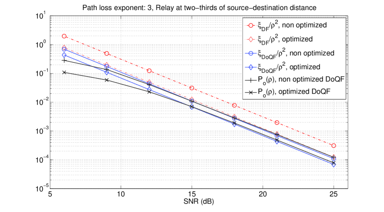
Figure 3: Outage performance of the DF and DoQF protocols

Figure 4 represents the outage gains for the DoQF and the DF versus $d_{0,1}$, the position of the relay on the source-destination line segment. Note from the figure that the farther the relay from the source is, the better DoQF compared to DF works. This fact can be explained as follows: If the relay is close to the destination, it will be more often in outage and the Quantization step will thus operate more often.

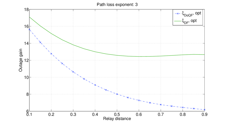
Figure 4: Outage gain of DF and DoQF versus relay position

In Figure 5, we plot the ratios of the outage gains with equal times and equal powers to the optimized outage gains as a function of the position $d_{0,1}$ of the relay on the source-destination segment. Note from this figure that optimizing the slots durations and the power allocation yields larger performance gains for both the DF and the DoQF when the relay is too close or too far from the source.

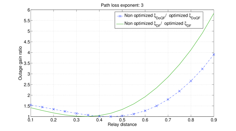
Figure 5: Outage gain of DF and DoQF versus relay position

In Figure  6, we plot the DMT of the DoQF (given by Theorem 3), orthogonal DF, (non-orthogonal) DF, NAF, DDF, and the MISO bound.

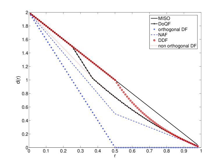
Figure 6: DMT of the DF and DoQF protocols

As already mentioned in a previous section, the DoQF outperforms the other static protocols. In contrast, the DDF protocol is still better than the DoQF but its dynamic approach leads to several implementation difficulties.

In Figure 7, the optimal sizes of slot 0 for the DoQF and the DF are plotted.

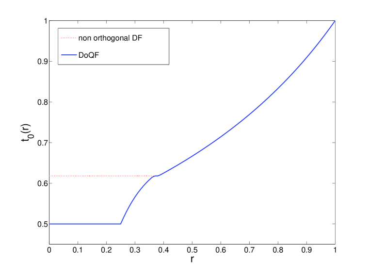
Figure 7: Optimal $t_{0}$ for DF and DoQF

We remark that, when $r$ is small enough, slots 0 and 1 have the same length. When $r$ increases, the duration of relay listening increases also. As a consequence, the duration of retransmission decreases. The duration for the quantization step thus decreases and the DoQF becomes closer to the DF as seen on the DMT.

VI Conclusions

A relaying protocol (DoQF) has been introduced for half-duplex single-relay scenarios. The proposed DoQF is a static relaying protocol that involves practical coding-decoding strategies at both the relay and the destination that can be implemented in practice. The performance of this protocol has been studied in the context of communications over slow fading wireless channels using two relevant performance metrics: The outage gain and the diversity multiplexing tradeoff (DMT). The DoQF protocol has been shown to be optimal in terms of outage gain in the wide class of half-duplex static relaying protocols. A method to minimize the outage gain of the DoQF w.r.t the slots durations and the power allocation has been also proposed. The proposed protocol has been finally shown to achieve the DMT of MISO for multiplexing gains $r\leq 0.25$. Some future research directions would be the extension of the proposed DoQF protocol to multi-relay networks and to networks involving frequency selective channels.

Appendix A Proof of Theorem 1

It is known [29] that the capacity of any static relaying protocol is limited by the cut-set upper-bound. In this appendix, we derive the outage gain associated with the cut-set capacity. We prove next that this outage gain is equal to $\xi_{\textrm{CS-HD}}$ given by (23).

The cut-set upper-bound on the capacity of any half-duplex single-relay protocol from the class $\mathcal{P}_{\textrm{HD}}(t_{0},\alpha_{0},\alpha_{1})$, with a listening time equal to $t_{0}T$ and a cooperation time equal to $(1-t_{0})T=t_{1}T$, is given by

$$C_{\textrm{CS-HD}}=\lim_{T\to\infty}\frac{1}{T}\max_{p(X_{00},X_{01},X_{11})}\min\big{\{}I(X_{00};Y_{10},Y_{20})+I(X_{01};Y_{21}|X_{11}),$$

$$I(X_{00};Y_{20})+I(X_{01},X_{11};Y_{21})\big{\}}\>,$$ (73)

where the maximization in (73) is with respect to all the joint distributions of $X_{00}$, $X_{01}$ and $X_{11}$ that satisfy the power constraints (21) and (22). It can be shown that the maximum in (73) is achieved when vectors $X_{00}$, $X_{01}$ and $X_{11}$ are zero-mean i.i.d Gaussian with covariance matrices that satisfy constraints (21) and (22). The cut-set upper-bound can thus be written as

$$C_{\textrm{CS-HD}}=\min\Big{\{} t_{0}\log\left(1+\mathbb{E}\left[|X_{0}(i)|^{2}\right]G_{01}+\mathbb{E}\left[|X_{0}(i)|^{2}\right]G_{02}\right)+t_{1}\log\left(1+\mathbb{E}\left[|X_{0}(i)|^{2}\right]G_{02}\right),$$

$$t_{0}\log\left(1+\mathbb{E}\left[|X_{0}(i)|^{2}\right]G_{02}\right)+t_{1}\log\left(1+\mathbb{E}\left[|X_{0}(i)|^{2}\right]G_{02}+\mathbb{E}\left[|X_{11}(i)|^{2}\right]G_{12}\right)\Big{\}}$$

$$=\min\{ C_{\textrm{SIMO}},C_{\textrm{MISO}}\}\>,$$ (74)

where $C_{\textrm{SIMO}}$ and $C_{\textrm{MISO}}$ are defined in order to simplify the presentation of the proof as follows:

$$C_{\textrm{SIMO}} =t_{0}\log\left(1+\mathbb{E}\left[|X_{0}(i)|^{2}\right]G_{01}+\mathbb{E}\left[|X_{0}(i)|^{2}\right]G_{02}\right)+t_{1}\log\left(1+\mathbb{E}\left[|X_{0}(i)|^{2}\right]G_{02}\right)$$

$$C_{\textrm{MISO}} =t_{0}\log\left(1+\mathbb{E}\left[|X_{0}(i)|^{2}\right]G_{02}\right)+t_{1}\log\left(1+\mathbb{E}\left[|X_{0}(i)|^{2}\right]G_{02}+\mathbb{E}\left[|X_{11}(i)|^{2}\right]G_{12}\right)\>.$$

We now prove that the limit $\lim_{\rho\to\infty}\rho^{2}\mathrm{Pr}[C_{\mathrm{CS-HD}}\leq R]$ exists and that it is equal to $\xi_{\mathrm{CS-HD}}$ given by (23). For that sake, note that the following holds:

$$\mathrm{Pr}[C_{\textrm{CS-HD}}\leq R]= 1-\mathrm{Pr}\left[C_{\textrm{CS-HD}}>R\right]$$

$$= 1-\mathrm{Pr}[C_{\textrm{SIMO}}>R,C_{\textrm{MISO}}>R]$$

$$\geq 1-\mathrm{Pr}\left[C_{\textrm{SIMO}}>R\right]\times\mathrm{Pr}\left[C_{\textrm{MISO}}>R\right]$$

$$= 1-\left(1-\mathrm{Pr}\left[C_{\textrm{SIMO}}\leq R\right]\right)\times\left(1-\mathrm{Pr}\left[C_{\textrm{MISO}}\leq R\right]\right)\>.$$

Now define

$$P_{o,\textrm{SIMO}} =\mathrm{Pr}\left[C_{\textrm{SIMO}}\leq R\right]$$

$$P_{o,\textrm{MISO}} =\mathrm{Pr}[C_{\textrm{MISO}}\leq R]\>.$$

Using these new notations, we conclude that the following lower-bound on $\mathrm{Pr}[C_{\textrm{CS-HD}}\leq R]$ holds:

$$\mathrm{Pr}[C_{\textrm{CS-HD}}\leq R]\geq P_{o,\textrm{SIMO}}+P_{o,\textrm{MISO}}-P_{o,\textrm{SIMO}}P_{o,\textrm{MISO}}\>.$$ (75)

In the same way, it is straightforward to show that $\mathrm{Pr}[C_{\textrm{CS-HD}}\leq R]$ can be upper-bounded as follows.

$$\mathrm{Pr}[C_{\textrm{CS-HD}}\leq R]\leq P_{o,\textrm{SIMO}}+P_{o,\textrm{MISO}}+P_{o,\textrm{SIMO}}P_{o,\textrm{MISO}}\>.$$ (76)

Now, we can use the same arguments and tools employed in Subsection III-D to prove that

$$\lim_{\rho\to\infty}\rho^{2}P_{o,\textrm{SIMO}}=\frac{c_{02}c_{01}}{\alpha_{0}^{2}}\int_{\mathbb{R}_{+}^{2}}\mathbf{1}\left\{t_{1}\log(1+u)+t_{0}\log\left(1+u+v\right)\leq R\right\}dudv$$ (77)

$$\lim_{\rho\to\infty}\rho^{2}P_{o,\textrm{MISO}}=\frac{c_{02}c_{12}}{\alpha_{0}\alpha_{1}}\int_{\mathbb{R}_{+}^{2}}\mathbf{1}\{t_{0}\log(1+u)+t_{1}\log(1+u+v)\leq R\}dudv$$ (78)

$$\lim_{\rho\to\infty}\rho^{2}P_{o,\textrm{SIMO}}P_{o,\textrm{MISO}}=0\>.$$ (79)

Note that the integrals in the rhs of (77) and (78) coincide with the two integrals in the rhs of (III-D). We can thus write

$$\lim_{\rho\to\infty}\rho^{2}P_{o,\textrm{SIMO}} =\frac{c_{02}c_{01}}{\alpha_{0}^{2}}\left(\frac{1}{2}+\frac{\exp(2R)}{4t_{0}-2}-\frac{t_{0}\exp(R/t_{0})}{2t_{0}-1}\right)$$ (80)

$$\lim_{\rho\to\infty}\rho^{2}P_{o,\textrm{MISO}} =\frac{c_{02}c_{12}}{\alpha_{01}\alpha_{02}}\left(\frac{1}{2}+\frac{\exp(2R)}{4t_{1}-2}-\frac{t_{1}\exp(R/t_{1})}{2t_{1}-1}\right)\>.$$ (81)

Combining (75), (76), (79), (80) and (81) we conclude that

$$\lim_{\rho\to\infty}\rho^{2}\mathrm{Pr}[C_{\textrm{CS-HD}}\leq RT]=\xi_{\mathrm{CS-HD}}\>,$$

where $\xi_{\textrm{CS-HD}}$ is the lower-bound defined by (23). Note that since $C_{\textrm{CS-HD}}$ is an upper-bound on the capacity of any static half-duplex relaying protocol belonging to the class $\mathcal{P}_{\textrm{HD}}(t_{0},\alpha_{0},\alpha_{1})$, then $\xi_{\textrm{CS-HD}}$ which satisfies $\xi_{CS-HD}=$ $\lim_{\rho\to\infty}$ $\rho^{2}\mathrm{Pr}[C_{\textrm{CS-HD}}\leq RT]$ is a lower-bound on the outage gain of any protocol from the class $\mathcal{P}_{\textrm{HD}}(t_{0},\alpha_{0},\alpha_{1})$. This completes the proof of Theorem 1.

Appendix B Derivation of $d_{2}(t_{0},\delta,r)$ (for $t_{0}\geq 0.5$ and $\delta>0$)

First, recall the definition of $d_{2}(t_{0},\delta,r)$ as $d_{2}(t_{0},\delta,r)=-\lim_{\rho\to\infty}\frac{\log(P_{o,2}(\rho))}{\log\rho}$, where the probability $P_{o,2}(\rho)$ is defined by (17) as

$$P_{o,2}(\rho)=\mathrm{Pr}\Bigg{[} t_{1}\log(1+\alpha_{0}\rho G_{02})+t_{0}\log\left(1+\alpha_{0}\rho G_{02}+\frac{\gamma(G_{01},\rho)\alpha_{0}\rho G_{01}}{\gamma(G_{01},\rho)+\Delta^{2}(\rho)\sqrt{\gamma(G_{01},\rho))}}\right)\leq R(\rho),$$

$$\overline{\mathcal{E}},\mathcal{F},\mathcal{S}\Bigg{]}\>,$$ (82)

where $\gamma(G_{01},\rho)=\frac{\left(1+\alpha_{0}\rho G_{01}-\Delta^{2}(\rho)\right)^{2}}{\left(1+\alpha_{0}\rho G_{01}\right)^{2}}$, and where events $\mathcal{E}$, $\mathcal{S}$ and $\mathcal{F}$ are defined by (4), (10) and (12) respectively. Note that $\gamma(G_{01},\rho)$ is positive since event $\mathcal{S}$ i.e., $1+\alpha_{0}\rho G_{01}\geq\Delta^{2}(\rho)$, is realized. Furthermore, we can check that the following result holds.

$$\frac{\gamma(G_{01},\rho)}{\gamma(G_{01},\rho)+\Delta^{2}(\rho)\sqrt{\gamma(G_{01},\rho)}}\stackrel{{\scriptstyle.}}{{=}}\frac{1}{1+\Delta^{2}(\rho)}\stackrel{{\scriptstyle.}}{{=}}\rho^{-(\delta)^{+}}\>.$$ (83)

In the following, we assume that $R(\rho)=r\log\rho$ in accordance with (1), and we define as in [22] the exponential order associated with channel $H_{ij}$ as $a_{ij}=-\frac{\log G_{ij}}{\log\rho}$. We can easily verify that $a_{ij}$ is a Gumbel distributed random variable with the probability density function $f_{a_{ij}}(a)=\log\rho\>e^{a}e^{-e^{-a\log\rho}}$. By plugging $G_{01}=\rho^{-a_{01}}$ into (4), the probability of the event $\overline{\mathcal{E}}$ i.e., $t_{0}\log(1+\alpha_{0}\rho G_{01})>R(\rho)$, can be written as

$$\mathrm{Pr}[\mathcal{E}]\dot{=}\mathrm{Pr}\left[\left(1-a_{01}\right)^{+}\leq\frac{r}{t_{0}}\right]\>.$$ (84)

Similarly, we can verify that the probability of event $\mathcal{F}$ i.e., $t_{1}\log\left(1+\frac{\phi(\rho)G_{12}}{\alpha_{0}\rho G_{02}+1}\right)>Q(\rho)t_{0}$, satisfies

$$\mathrm{Pr}[\mathcal{F}]\dot{=}\mathrm{Pr}\left[\left(1+\left(1-\frac{r}{t_{0}}\right)^{+}-a_{12}-(1-a_{02})^{+}\right)^{+}\leq\frac{r}{t_{1}}-\frac{t_{0}}{t_{1}}\delta\right]\>,$$ (85)

and that the probability of $\mathcal{S}$ satisfies

$$\mathrm{Pr}[\mathcal{S}]\dot{=}\mathrm{Pr}[\delta\leq\left(1-a_{01}\right)^{+}]\>.$$ (86)

By plugging $R(\rho)=r\log\rho$, $G_{01}=\rho^{-a_{01}}$, $G_{02}=\rho^{-a_{02}}$, $G_{12}=\rho^{-a_{12}}$, (83), (84), (85) and (86) into (82), the following high SNR result holds for $\delta>0$.

$$P_{o,2}(\rho)\dot{=}\mathrm{Pr}\Bigg{[} t_{1}(1-a_{02})^{+}+t_{0}(1-\min(a_{02},a_{01}+\delta))^{+}<r\>,\>(1-a_{01})^{+}<\frac{r}{t_{0}}\>,$$

$$\>\left(1+\left(1-\frac{r}{t_{0}}\right)^{+}-a_{12}-(1-a_{02})^{+}\right)^{+}>\frac{r}{t_{1}}-\frac{t_{0}}{t_{1}}\delta\>,\>\delta\leq\left(1-a_{01}\right)^{+}\Bigg{]},$$ (87)

or, equivalently,

$$P_{o,2}(\rho)\dot{=}\int_{\mathcal{O}}f_{a_{01}}(a_{01})f_{a_{02}}(a_{02})f_{a_{12}}(a_{12})da_{01}da_{02}da_{12}\>,$$ (88)

where $f_{a_{ij}}(.)$ is the probability density function of $a_{ij}$ and

$$\mathcal{O}=\Bigg{\{} (a_{01},a_{02},a_{12})\in\mathbb{R}^{3}\>|\>t_{1}(1-a_{02})^{+}+t_{0}(1-\min(a_{02},a_{01}+\delta))^{+}<r\>,\>(1-a_{01})^{+}<\frac{r}{t_{0}}\>,$$

$$\>\left(1+\left(1-\frac{r}{t_{0}}\right)^{+}-a_{12}-(1-a_{02})^{+}\right)^{+}>\frac{r}{t_{1}}-\frac{t_{0}}{t_{1}}\delta\>,\>\delta\leq\left(1-a_{01}\right)^{+}\Bigg{\}}\>.$$ (89)

Plugging the expression of $f_{a_{ij}}(.)$ given earlier into (88), $P_{o,2}(\rho)$ can be written as

$$P_{o,2}(\rho)\dot{=}\int_{\cal O}(\log\rho)^{3}\rho^{-(a_{01}+a_{02}+a_{12})}e^{-\rho^{-a_{01}}}e^{-\rho^{-a_{02}}}e^{-\rho^{-a_{12}}}da_{01}da_{02}da_{12}\>.$$

It can be shown (refer to [22]) that the term $(\log\rho)^{3}$ can be dropped from the latter equation without losing its exactness. Moreover, integration in the same equation can be restricted to positive values of $a_{01}$, $a_{02}$ and $a_{12}$. Define $\mathcal{O}_{+}=\mathcal{O}\cap\mathbb{R}_{+}^{3}$. The probability $P_{o,2}(\rho)$ thus satisfies

$$P_{o,2}(\rho)\dot{=}\int_{\mathcal{O}_{+}}\rho^{-(a_{01}+a_{02}+a_{12})}da_{01}da_{02}da_{12}\>,$$ (90)

and the DMT $d_{2}(t_{0},\delta,r)$ associated with $P_{o,2}(\rho)$ can now be written [22] as

$$d_{2}(t_{0},\delta,r)=\inf_{(a_{01},a_{02},a_{12})\in{{\cal O}^{+}}}(a_{01}+a_{02}+a_{12})\>.$$ (91)

In this appendix, the derivation of $d_{2}(t_{0},\delta,r)$ will be done only in the case characterized by $t_{0}\geq 0.5$ and $\delta>0$. The derivation in the case $\delta\leq 0$ or $t_{0}<0.5$ follows the same approach.

Consider first the case $0<\delta\leq 1-\left(1-\frac{r}{t_{0}}\right)^{+}$. The infimum in (91) can be computed by partitioning ${\cal O}_{+}$ into subsets according to whether $a_{01}$, $a_{02}$ are smaller or larger than 1.

• $\boldsymbol{a_{01}>1}$. In this case, $(1-a_{01})^{+}=0$ and the fourth inequality in (B) reduces to $\delta\leq 0$. This result contradicts our assumption that $\delta>0$. There is therefore no triples $(a_{01},a_{02},a_{12})\in{\cal O}^{+}$ such that $a_{01}>1$.

• $\boldsymbol{a_{01}\leq 1,a_{02}>1}$. Since the third inequality in the definition of $\cal O$ given by (B) contains the term $\left(1+\left(1-\frac{r}{t_{0}}\right)^{+}-a_{12}-(1-a_{02})^{+}\right)^{+}$, then we should consider two categories of triples $(a_{01},a_{02},a_{12})$:

  • $1+\left(1-\frac{r}{t_{0}}\right)^{+}-a_{12}-(1-a_{02})^{+}<0$.
    For triples $(a_{01},a_{02},a_{12})\in{\cal O}^{+}$ under this category, the third inequality in (B) can be reduced to $\delta>\frac{r}{t_{0}}$, which contradicts the second and the fourth inequalities in (B). This category can be therefore dropped out.

  • $1+\left(1-\frac{r}{t_{0}}\right)^{+}-a_{12}-(1-a_{02})^{+}\geq 0$.
    Recall the first inequality in (B) i.e., $t_{1}(1-a_{02})^{+}+t_{0}(1-\min(a_{02},a_{01}+\delta))^{+}<r$. Since $\delta\leq(1-a_{01})^{+}$ due to the fourth inequality in (B), then $a_{01}+\delta\leq a_{01}+(1-a_{01})^{+}=1\leq a_{02}$. The first inequality in (B) reduces thus to $a_{01}\geq\left(1-\frac{r}{t_{0}}\right)^{+}$. We conclude that

    $$\inf_{a_{01}\leq 1,a_{02}>1}(a_{01}+a_{02}+a_{12})=1+\left(1-\frac{r}{t_{0}}\right)^{+}\>.$$ (92)

    One can verify after some simple algebra that $\inf_{a_{01}\leq 1,a_{02}>1}(a_{01}+a_{02}+a_{12})=1+\left(1-\frac{r}{t_{0}}\right)^{+}$ is always larger than $d_{1}(t_{0},r)$ given by (58). Therefore, the term $\inf_{a_{01}\leq 1,a_{02}>1}(a_{01}+a_{02}+a_{12})$ never coincides with the minimum in $d(t_{0},\delta,r)=\min\{d_{1}(t_{0},r)$, $d_{2}(t_{0},\delta,r)$,$d_{3}(t_{0},\delta,r)$, $d_{4}(t_{0},\delta,r)\}$. As a result, the argument of the infimum $\inf_{(a_{01},a_{02},a_{12})\in{{\cal O}_{+}}}(a_{01}+a_{02}+a_{12})$ coincides necessarily with a triple $(a_{01},a_{02},a_{12})$ from the following subset.

• $\boldsymbol{a_{01}\leq 1,a_{02}\leq 1}$. Two categories of triples $(a_{01},a_{02},a_{12})$ should be considered.

  • $1+\left(1-\frac{r}{t_{0}}\right)^{+}-a_{12}-(1-a_{02})^{+}<0$.
    As done before, it is straightforward to verify that there is no triples $(a_{01},a_{02},a_{12})\in{\cal O}^{+}$ that fall under this category.

  • $1+\left(1-\frac{r}{t_{0}}\right)^{+}-a_{12}-(1-a_{02})^{+}\geq 0$.
    The third inequality in (B) leads in this case to

    $$a_{02}>\frac{r}{t_{1}}-\left(1-\frac{r}{t_{0}}\right)^{+}-\frac{t_{0}}{t_{1}}\delta\>.$$ (93)

    In order to evaluate the first inequality in (B), two subcategories of triples $(a_{01},a_{02},a_{12})$ should be further examined.

    1. $a_{02}<a_{01}+\delta$. For triples $(a_{01},a_{02},a_{12})\in{\cal O}^{+}$ under this category, the first inequality in (B) leads to $a_{02}>(1-r)^{+}$.

    2. $a_{02}\geq a_{01}+\delta$. The first inequality results in this case in $a_{02}+\frac{t_{0}}{t_{1}}a_{01}>\frac{1-r}{t_{1}}-\frac{t_{0}}{t_{1}}\delta$.

    Referring to Figures 9 and 9 reveals that $\inf_{a_{01}\leq 1,a_{02}\leq 1}(a_{01}+a_{02}+a_{12})$ coincides with the rhs of (IV-D). We have thus proved that $d_{2}(t_{0},\delta,r)$ is indeed given by (IV-D).

Figure 8: Outage region for the DoQF protocol in the case $\frac{r}{t_{1}}-\left(1-\frac{r}{t_{0}}\right)^{+}$ $-\frac{t_{0}}{t_{1}}\delta\leq 1-r$.

Figure 9: Outage region for the DoQF protocol in the case $1-r<\frac{r}{t_{1}}-\left(1-\frac{r}{t_{0}}\right)^{+}-\frac{t_{0}}{t_{1}}\delta$.

Now consider the case $\delta>1-\left(1-\frac{r}{t_{0}}\right)^{+}$ in order to prove that (62) holds. To that end, refer to the second and the fourth inequalities in the definition of $\mathcal{O}$ given by (B), that is $(1-a_{01})^{+}<\frac{r}{t_{0}}$ and $\delta\leq(1-a_{01})^{+}$. Note that $(1-a_{01})^{+}\leq 1$ since $a_{01}>0$. A necessary condition for $a_{01}$ to satisfy the second and the fourth inequalities in (B), and consequently to belong to $\mathcal{O}_{+}$ is thus $\delta\leq\min\left\{1,\frac{r}{t_{0}}\right\}=1-\left(1-\frac{r}{t_{0}}\right)^{+}$. This means that if we choose $\delta$ such that $\delta>1-\left(1-\frac{r}{t_{0}}\right)^{+}$, the set $\mathcal{O}_{+}$ will be empty. In this case, $P_{o,2}(\rho)=0$ for sufficiently large $\rho$. In other words, there exists $\rho_{0}>0$ such that $\forall\rho\geq\rho_{0}$, the event $\overline{\mathcal{E}}\&\mathcal{S}$ cannot be realized and the relay will not be able to quantize, reducing the DoQF to a classical DF scheme. The corresponding DMT $d_{2}(t_{0},\delta,r)$ will have no effect in this case on the final DMT of the protocol. We can give it for convenience the value $d_{2}(t_{0},\delta,r)=2(1-r)^{+}$, which is the upper-bound on the DMT of any single-relay protocol.

Appendix C Derivation of $d_{\mathrm{DoQF}}^{*}(r)=\sup_{\delta,t_{0}}d(t_{0},\delta,r)$

Before proceeding with the proof, it is useful to recall here the definition of $t_{0,{\mathrm{DoQF}}}^{*}(r)$ and $\delta_{\mathrm{DoQF}}^{*}(r)$ as the argument of the supremum in $d_{\mathrm{DoQF}}^{*}(r)=\sup_{\delta,t_{0}}d(t_{0},\delta,r)$.

We will first compute $d_{\mathrm{DoQF}}^{*}(r)$ in the case $r\leq 0.25$, and then in the case $r>0.25$.

The case $\boldsymbol{r\leq 0.25}$

Let us plug $t_{0}=0.5$ and $\delta=0$ into (58), (IV-D), (69) and (72) to obtain

$$d_{1}(t_{0},r)=d_{2}(t_{0},\delta,r)=d_{4}(t_{0},\delta,r)=2(1-r)^{+}\>,$$ (94)

$$d_{3}(t_{0},\delta,r)=2(1-2r)^{+}+\left(2(1-2r)^{+}-2r\right)^{+}=2-8r\>.$$ (95)

Note that $d_{3}(t_{0},\delta,r)$ is the only term that may be different from $2(1-r)^{+}$. However, one can verify by referring to (95) that $d_{3}(t_{0},\delta,r)\geq 2(1-r)^{+}\>\Leftrightarrow\>r\leq 0.25$. We conclude that, for $r\leq 0.25$, $d(0.5,0,r)=2(1-r)^{+}$. We have thus proved that the MISO upper-bound is achieved by the DoQF for $r\leq 0.25$ by choosing $t_{0,\textrm{DoQF}}^{*}(r)=0.5$ and $\delta_{\textrm{DoQF}}^{*}(r)=0$.

The case $\boldsymbol{r>0.25}$

The first step of the proof in this case is to reduce the size of the set of possible values of $t_{0,{\mathrm{DoQF}}}^{*}(r)$ and $\delta_{\mathrm{DoQF}}^{*}(r)$. We will prove in particular that the following three lemmas hold.

Lemma 1.

For any $r\in[0,1]$, $d_{\mathrm{DoQF}}^{*}(r)\geq d_{\mathrm{DF}}^{*}(r)$.

In other words, Lemma 1 states that the DMT achieved by the DoQF protocol cannot be worse than the DMT achieved by the DF. The proof of Lemma 1 is given in Appendix D-A.

Lemma 2.

For any $r\in[0,1]$, the following inequalities hold true: $\max\{0.5,r\}\leq t_{0,{\mathrm{DoQF}}}^{*}(r)\leq t_{0,{\mathrm{DF}}}^{*}(r)$.

Here, $t_{0,{\mathrm{DF}}}^{*}(r)$ is the value of $t_{0}$ defined by (54) which allows to achieve the DMT of the DF protocol. The proof of Lemma 2 is given in Appendix D-B.

Lemma 3.

Assume that $r>0.25$. The following holds true: $0<\delta_{\mathrm{DoQF}}^{*}(r)<1-\left(1-\frac{r}{t_{0,{\mathrm{DoQF}}}^{*}(r)}\right)^{+}$.

The proof of Lemma 3 is given in Appendix D-C.

These three lemmas will considerably simplify the derivation of $d_{\mathrm{DoQF}}^{*}(r)$. Indeed, with the help of Lemma 2 and Lemma 3, we will derive the DMT of the DoQF firstly in the case when $0.25<r\leq\frac{2(\sqrt{5}-1)}{9-\sqrt{5}}$, and secondly in the case when $\frac{2(\sqrt{5}-1)}{9-\sqrt{5}}<r\leq 1$.

• $0.25<r\leq\frac{2(\sqrt{5}-1)}{9-\sqrt{5}}$.
  We begin with the simplification of the DMT terms $d_{1}\left(t_{0,{\textrm{DoQF}}}^{*}(r),r\right)$, $d_{2}\left(t_{0,{\textrm{DoQF}}}^{*}(r),\delta_{\textrm{DoQF}}^{*}(r),r\right)$, $d_{3}\left(t_{0,{\textrm{DoQF}}}^{*}(r),\delta_{\textrm{DoQF}}^{*}(r),r\right)$ and $d_{4}\left(t_{0,{\textrm{DoQF}}}^{*}(r),\delta_{\textrm{DoQF}}^{*}(r),r\right)$. The final DMT $d_{\textrm{DoQF}}^{*}(r)$ can then be deduced as the minimum of the above terms. Consider first the derivation of $d_{1}\left(t_{0,{\textrm{DoQF}}}^{*}(r),r\right)$. Since Lemma 2 states that $t_{0,{\textrm{DoQF}}}^{*}(r)\leq t_{0,{\textrm{DF}}}^{*}(r)=\frac{2}{\sqrt{5}+1}$, it follows from (58) that

  $$d_{1}\left(t_{0,{\textrm{DoQF}}}^{*}(r),r\right)=2-\frac{r}{1-t_{0,{\textrm{DoQF}}}^{*}(r)}\>.$$ (96)

  We now proceed to the simplification of the expression of $d_{2}\left(t_{0,{\textrm{DoQF}}}^{*}(r),\delta_{\textrm{DoQF}}^{*}(r),r\right)$. Thanks to Lemma 2 and Lemma 3, we will prove that

  $$d_{2}\left(t_{0,{\textrm{DoQF}}}^{*}(r),\delta_{\textrm{DoQF}}^{*}(r),r\right)=(1-r)^{+}+\max\left\{1-\frac{r}{t_{0,{\textrm{DoQF}}}^{*}(r)},1-r-\delta_{\textrm{DoQF}}^{*}(r)\right\}\>.$$ (97)

  For that sake, refer to (IV-D) and note that proving (97) is equivalent to proving that

  $$\frac{r}{1-t_{0,{\textrm{DoQF}}}^{*}(r)}-\left(1-\frac{r}{t_{0,{\textrm{DoQF}}}^{*}(r)}\right)^{+}-\frac{t_{0,{\textrm{DoQF}}}^{*}(r)}{1-t_{0,{\textrm{DoQF}}}^{*}(r)}\delta_{\textrm{DoQF}}^{*}(r)\leq 1-r\>.$$ (98)

  In order to show that (98) holds, we suppose to the contrary that $\frac{r}{1-t_{0,{\textrm{DoQF}}}^{*}(r)}-\left(1-\frac{r}{t_{0,{\textrm{DoQF}}}^{*}(r)}\right)^{+}-\frac{t_{0,{\textrm{DoQF}}}^{*}(r)}{1-t_{0,{\textrm{DoQF}}}^{*}(r)}\delta_{\textrm{DoQF}}^{*}(r)>1-r$. Since $\delta_{\textrm{DoQF}}^{*}(r)>0$ according to Lemma 3, the latter assumption leads to

  $$r>\frac{2t_{0,{\textrm{DoQF}}}^{*}(r)\left(1-t_{0,{\textrm{DoQF}}}^{*}(r)\right)}{1+t_{0,{\textrm{DoQF}}}^{*}(r)\left(1-t_{0,{\textrm{DoQF}}}^{*}(r)\right)}\>.$$ (99)

  Moreover, it is straightforward to show that

  $$\min_{0.5\leq t\leq\frac{2}{\sqrt{5}+1}}\frac{2t\left(1-t\right)}{1+t\left(1-t\right)}>\frac{2(\sqrt{5}-1)}{9-\sqrt{5}}\>,$$ (100)

  where the restriction to $0.5\leq t\leq t_{0,{\textrm{DF}}}^{*}(r)=\frac{2}{\sqrt{5}+1}$ is due to Lemma 2. Now, we can combine (99) and (100) in order to get $r>\frac{2(\sqrt{5}-1)}{9-\sqrt{5}}\>,$ which contradicts the fact that $r\leq\frac{2(\sqrt{5}-1)}{9-\sqrt{5}}$. We conclude that expression (97) holds true.

  We can further simplify the expression (97) by proving that $1-r-\delta_{\textrm{DoQF}}^{*}(r)\geq 1-\frac{r}{t_{0,{\textrm{DoQF}}}^{*}(r)}$. The proof of this point uses the same arguments as above and is thus omitted. The term $d_{2}\left(t_{0,{\textrm{DoQF}}}^{*}(r),\delta_{\textrm{DoQF}}^{*}(r),r\right)$ can finally be written as

  $$d_{2}\left(t_{0,{\textrm{DoQF}}}^{*}(r),\delta_{\textrm{DoQF}}^{*}(r),r\right)=2(1-r)^{+}-\delta_{\textrm{DoQF}}^{*}(r)\>.$$ (101)

  As for $d_{3}\left(t_{0,{\textrm{DoQF}}}^{*}(r),\delta_{\textrm{DoQF}}^{*}(r),r\right)$ given by (69), it simplifies to

  $$d_{3}\left(t_{0,{\textrm{DoQF}}}^{*}(r),\delta_{\textrm{DoQF}}^{*}(r),r\right)=4+\frac{t_{0,{\textrm{DoQF}}}^{*}(r)}{1-t_{0,{\textrm{DoQF}}}^{*}(r)}\delta_{\textrm{DoQF}}^{*}(r)-\left(4+\frac{t_{0,{\textrm{DoQF}}}^{*}(r)}{1-t_{0,{\textrm{DoQF}}}^{*}(r)}\right)\frac{r}{t_{0,{\textrm{ DoQF}}}^{*}(r)}$$ (102)

  The remaining task is to simplify the expression (72) which defines $d_{4}\left(t_{0,{\textrm{DoQF}}}^{*}(r),\delta_{\textrm{DoQF}}^{*}(r),r\right)$. For that sake, we can resort to Lemma 1 to prove that

  $$d_{4}\left(t_{0,{\textrm{DoQF}}}^{*}(r),\delta_{\textrm{DoQF}}^{*}(r),r\right)=(1-r)^{+}+(1-\delta_{\textrm{DoQF}}^{*}(r))\>.$$

  It follows that $d_{4}\left(t_{0,{\textrm{DoQF}}}^{*}(r),\delta_{\textrm{DoQF}}^{*}(r),r\right)\geq d_{2}\left(t_{0,{\textrm{DoQF}}}^{*}(r),\delta_{\textrm{DoQF}}^{*}(r),r\right)$ and that it can thus be dropped from the derivation of the final DMT of the DoQF. Now that the DMT terms $d_{1}\left(t_{0,{\textrm{DoQF}}}^{*}(r),r\right)$, $d_{2}\left(t_{0,{\textrm{DoQF}}}^{*}(r),\delta_{\textrm{DoQF}}^{*}(r),r\right)$ and $d_{3}\left(t_{0,{\textrm{DoQF}}}^{*}(r),\delta_{\textrm{DoQF}}^{*}(r),r\right)$ have been expressed as functions of $t_{0,{\textrm{DoQF}}}^{*}(r)$ and $t_{0,{\textrm{DoQF}}}^{*}(r)$, we can proceed to the determination of $t_{0,{\textrm{DoQF}}}^{*}(r)$, $\delta_{\textrm{DoQF}}^{*}(r)$, and consequently $d_{\textrm{DoQF}}^{*}(r)$.

  • Determination of $\delta_{\textrm{DoQF}}^{*}(r)$:

    Assume that $t_{0,{\textrm{DoQF}}}^{*}(r)$ has been already determined. It is straightforward to verify that $d_{2}\left(t,\delta,r\right)$ given by (101) is decreasing w.r.t $\delta$, and that $d_{3}\left(t,\delta,r\right)$ given by (102) is increasing w.r.t $\delta$ on $\mathbb{R}^{+}$. Furthermore, $d_{2}\left(t,0,r\right)>d_{3}\left(t,0,r\right)$. We conclude that

    $$d_{2}\left(t_{0,{\textrm{DoQF}}}^{*}(r),\delta_{\textrm{DoQF}}^{*}(r),r\right)=d_{3}\left(t_{0,{\textrm{DoQF}}}^{*}(r),\delta_{\textrm{DoQF}}^{*}(r),r\right)\>.$$

    Therefore, $\delta_{\textrm{DoQF}}^{*}(r)$ can be given as a function of $t_{0,{\textrm{DoQF}}}^{*}(r)$ as follows

    $$\delta_{\textrm{DoQF}}^{*}(r)=\left(4-3t_{0,{\textrm{DoQF}}}^{*}(r)\right)\frac{r}{t_{0,{\textrm{DoQF}}}^{*}(r)}-(2+2r)\left(1-t_{0,{\textrm{DoQF}}}^{*}(r)\right)\>,$$ (103)

    which leads to

    $$d_{2}\left(t_{0,{\textrm{DoQF}}}^{*}(r),\delta_{\textrm{DoQF}}^{*}(r),r\right)=d_{3}\left(t_{0,{\textrm{DoQF}}}^{*}(r),\delta_{\textrm{DoQF}}^{*}(r),r\right)=$$

    $$2-2r+(2+2r)\left(1-t_{0,{\textrm{DoQF}}}^{*}(r)\right)-\left(4-3t_{0,{\textrm{DoQF}}}^{*}(r)\right)\frac{r}{t_{0,{\textrm{DoQF}}}^{*}(r)}\>.$$ (104)

  • Determination of $t_{0,\textrm{DoQF}}^{*}(r)$:

    We can show in the same way that $t_{0,{\textrm{DoQF}}}^{*}(r)$ can be obtained by writing

    $$d_{1}\left(t_{0,{\textrm{DoQF}}}^{*}(r),r\right)=d_{2}\left(t_{0,{\textrm{DoQF}}}^{*}(r),\delta_{\textrm{DoQF}}^{*}(r),r\right)\>.$$ (105)

    Plugging the expression of $\delta_{\textrm{DoQF}}^{*}(r)$ from (103) and the expression of $d_{2}\Big{(}t_{0,{\textrm{DoQF}}}^{*}(r)$, $\delta_{\textrm{DoQF}}^{*}(r)$, $r\Big{)}$ from (104) into (105) leads to equation (42) given in Theorem 3 as

    $$2(1+r)t_{0,{\textrm{DoQF}}}^{*}(r)^{3}-(4+5r)t_{0,{\textrm{DoQF}}}^{*}(r)^{2}+2(1+4r)t_{0,{\textrm{DoQF}}}^{*}(r)-4r=0\>.$$

    It can be shown after some algebra that the above equation admits a unique solution $v^{*}(r)$ on $\left[0.5,\frac{2}{\sqrt{5}+1}\right]$ provided that $r\leq\frac{2(\sqrt{5}-1)}{9-\sqrt{5}}$. This explains why the distinction $r\leq\frac{2(\sqrt{5}-1)}{9-\sqrt{5}}$ and $r>\frac{2(\sqrt{5}-1)}{9-\sqrt{5}}$ appears in Theorem 3. Once the solution $v^{*}(r)$ to the above equation has been computed, then $d_{\textrm{DoQF}}^{*}(r)$, $t_{0,{\textrm{DoQF}}}^{*}(r)$ and $\delta_{\textrm{DoQF}}^{*}(r)$ given respectively by (41), (47) and (51) can be easily obtained.

• $\frac{2(\sqrt{5}-1)}{9-\sqrt{5}}<r\leq 1$.
  In this case, we need to prove that $d_{\textrm{DoQF}}^{*}(r)=d_{\textrm{DF}}^{*}(r)$. To that end, we can show that $d_{\textrm{DoQF}}^{*}(r)>d_{\textrm{DF}}^{*}(r)$ leads to a contradiction. The proof of this point is based on Lemmas 1, 2 and 3 and is omitted due to lack of space.

The proof of Theorem 3 is thus completed.

Appendix D Proofs of Lemmas 1, 2, and 3

D-A Proof of Lemma 1

Assume that parameters $t_{0}$ and $\delta$ of the DoQF protocol are fixed such that $t_{0}=t_{0,\textrm{DF}}^{*}(r)$ and $\delta=1-\left(1-\frac{r}{t_{\textrm{DF}}^{*}(r)}\right)^{+}=\frac{r}{t_{\textrm{DF}}^{*}(r)}$, where $t_{0,\textrm{DF}}^{*}(r)$ is defined by (54). In this case, equations (58), (IV-D), (69) and (72) lead to $d_{1}(t_{0},r)=d_{4}(t_{0},\delta,r)=d_{\textrm{DF}}^{*}(r)$ and $d_{2}(t_{0},\delta,r)=d_{3}(t_{0},\delta,r)=2(1-r)^{+}$, meaning that $d(t_{0},\delta,r)=d_{\textrm{DF}}^{*}(r)$.

We conclude that the DoQF can be reduced to have the performance of DF by choosing $t_{0}=t_{0,\textrm{DF}}^{*}(r)$ and $\delta=\frac{r}{t_{0,\textrm{DF}}^{*}(r)}$. The final DMT $d_{\textrm{DoQF}}^{*}(r)$ of the DoQF is therefore necessarily greater or equal to $d_{\textrm{DF}}^{*}(r)$. The proof of Lemma 1 is thus completed.

D-B Proof of Lemma 2

Proving Lemma 2 requires proving that the following three inequalities hold: $r\leq t_{0,\textrm{DoQF}}^{*}(r)$, $t_{0,\textrm{DoQF}}^{*}(r)$ $\leq t_{0,\textrm{DF}}^{*}(r)$ and $0.5\leq t_{0,\textrm{DoQF}}^{*}(r)$. Let us begin with the proof of the inequality $r\leq t_{0,\textrm{DoQF}}^{*}(r)$. Assume to the contrary that $r>t_{0,\textrm{DoQF}}^{*}(r)$. In this case, $d_{3}(t_{0,\textrm{DoQF}}^{*}(r),\delta_{\textrm{DoQF}}^{*}(r),r)=0$ due to (69). This implies that the DMT of the DoQF satisfies $d(t_{0,\textrm{DoQF}}^{*}(r),\delta_{\textrm{DoQF}}^{*}(r),r)=d_{3}(t_{0,\textrm{DoQF}}^{*}(r),\delta_{\textrm{DoQF}}^{*}(r),r)=0$, which is in contradiction with Lemma 1. We conclude that $r\leq t_{0,\textrm{DoQF}}^{*}(r)$ holds true.

We now show that the inequality $t_{0,\textrm{DoQF}}^{*}(r)\leq t_{0,\textrm{DF}}^{*}(r)$ also holds true. For that sake, note that the DMT $d_{\textrm{DF}}^{*}(r)$ of DF given by (53) can be written as a function of $t_{0,\textrm{DF}}^{*}(r)$ defined by (54):

$$d_{\textrm{DF}}^{*}(r)=2-\frac{r}{1-t_{0,\textrm{DF}}^{*}(r)}=d_{1}\left(t_{0,\textrm{DF}}^{*}(r),r\right)\>,$$ (106)

where the second equality in (106) can be easily checked by referring to (58). On the other hand,

$$d_{1}\left(t_{0,\textrm{DoQF}}^{*}(r),r\right)\geq d_{\textrm{DoQF}}^{*}(r)$$ (107)

due to (56). Furthermore, Lemma 1 states that

$$d_{\textrm{DoQF}}^{*}(r)\geq d_{\textrm{DF}}^{*}(r)\>.$$ (108)

Combining (106), (107) and (108) leads to $d_{1}\left(t_{0,\textrm{DoQF}}^{*}(r),r\right)\geq d_{1}\left(t_{0,\textrm{DF}}^{*}(r),r\right)$. Since $d_{1}(t_{0},r)=2-\frac{r}{1-t_{0}}$, we conclude that $t_{0,\textrm{DoQF}}^{*}(r)\leq t_{0,\textrm{DF}}^{*}(r)$ holds.

In order to prove that inequality $t_{0,\textrm{DoQF}}^{*}(r)\geq 0.5$ holds, we will show that the best DMT that can be achieved with $t_{0}<0.5$ i.e., $\max_{t_{0}<0.5}d(t_{0},\delta,r)$, is less or equal to the DMT that can be achieved by choosing $t_{0}\geq 0.5$. It can be shown after some algebra that

$$\forall u\geq 0.5,\forall v<0.5,\>\>\>\>d_{2}(v,\delta,r)\leq d_{2}(u,\delta,r)\>,$$

where $d_{2}(u,\delta,r)$ is given by (IV-D) and $d_{2}(v,\delta,r)$ is given by (IV-D). Furthermore, it is straightforward to show that functions $t\mapsto d_{3}(t,\delta,r)$ and $t\mapsto d_{4}(t,\delta,r)$ defined respectively by (69) and (72) are increasing w.r.t $t$. Finally, since $d_{1}(v,r)=2(1-r)^{+}$ for any $v<0.5$ due to (58), then $d(v,\delta,r)=\min\{d_{2}(v,\delta,r),d_{3}(v,\delta,r),d_{4}(v,\delta,r)\}$. Putting all pieces together, we conclude that

$$\forall u\geq 0.5,\forall v<0.5,\>\>\>\>d(v,\delta,r)\leq d(u,\delta,r)\>,$$

which in turn means that $t_{0,\textrm{DoQF}}^{*}\geq 0.5$.

D-C Proof of Lemma 3

Lemma 3 states that the following two inequalities hold true for $r>0.25$:

$\delta_{\mathrm{DoQF}}^{*}(r)<1-\left(1-\frac{r}{t_{0,{\textrm{DoQF}}}^{*}(r)}\right)^{+}$ and $0<\delta_{\mathrm{DoQF}}^{*}(r)$.

Recall from our discussion in Appendix B that the first inequality is a necessary condition for the DMT of the DoQF protocol to be greater or equal to the DMT of DF. We thus only need to prove the second inequality. To that end, we will resort to Lemma 1 which implies that

$$d_{3}\left(t_{0,{\textrm{DoQF}}}^{*}(r),\delta_{\textrm{DoQF}}^{*}(r),r\right)\geq d_{\textrm{DF}}^{*}(r)\>,$$ (109)

where $d_{3}\left(t_{0,{\textrm{DoQF}}}^{*}(r),\delta_{\textrm{DoQF}}^{*}(r),r\right)=4+\frac{t_{0,{\textrm{DoQF}}}^{*}(r)}{1-t_{0,{\textrm{DoQF}}}^{*}(r)}\delta_{\textrm{DoQF}}^{*}(r)-\left(4+\frac{t_{0,{\textrm{DoQF}}}^{*}(r)}{1-t_{0,{\textrm{DoQF}}}^{*}(r)}\right)\frac{r}{t_{0,{\textrm{ DoQF}}}^{*}(r)}$ due to (102). Consider first the case $\frac{\sqrt{5}-1}{\sqrt{5}+1}<r\leq 1$. In this case, $d_{\textrm{DF}}^{*}(r)=(1-r)(2-r)$ due to [23]. Inequality (109) is therefore equivalent to

$$4+\frac{t_{0,{\textrm{DoQF}}}^{*}(r)}{1-t_{0,{\textrm{DoQF}}}^{*}(r)}\delta_{\textrm{DoQF}}^{*}(r)-\left(4+\frac{t_{0,{\textrm{DoQF}}}^{*}(r)}{1-t_{0,{\textrm{DoQF}}}^{*}(r)}\right)\frac{r}{t_{0,{\textrm{ DoQF}}}^{*}(r)}\geq(1-r)(2-r)\>.$$

It is straightforward to show that the above inequality is equivalent to

$$\frac{t_{0,{\textrm{DoQF}}}^{*}(r)}{1-t_{0,{\textrm{DoQF}}}^{*}(r)}\delta_{\textrm{DoQF}}^{*}(r)\geq r^{2}+\left(\frac{4}{t_{0,{\textrm{DoQF}}}^{*}(r)}+\frac{1}{1-t_{0,{\textrm{DoQF}}}^{*}(r)}-3\right)r-2\>.$$ (110)

One can check after some algebra that the rhs of (110) is strictly positive for $\frac{\sqrt{5}-1}{\sqrt{5}+1}<r\leq 1$. We conclude that $\delta_{\textrm{DoQF}}^{*}(r)>0$ on this interval. The proof of the strict positivity of $\delta_{\textrm{DoQF}}^{*}(r)$ for $0.25<r\leq\frac{\sqrt{5}-1}{\sqrt{5}+1}$ can be done without difficulty in the same way, completing the proof of Lemma 3.

References

• [1] R. U. Nabar, H. Bölcskei and F. W. Kneubühler, “Fading relay channels: Performance limits and space-time signal design,” IEEE Journal on Selected Areas of Communications, vol. 22, no. 6, pp. 1099-1109, Aug. 2004.
• [2] S. Yang and J.-C. Belfiore, “Towards the optimal amplify-and-forward cooperative diversity scheme,” IEEE Trans. on Information Theory, vol. 53, no. 9, pp. 3114-3126, Sep. 2007.
• [3] M. Katz and S. Shamai, “Relaying protocols for two colocated users,” IEEE Trans. on Information Theory, vol. 52, no. 6, pp. 2329-2344, June 2006.
• [4] J. N. Laneman, D. N. Tse and G. W. Wornell, “Cooperative diversity in wireless networks: Efficient protocols and outage behavior,” IEEE Trans. on Information Theory, vol. 50, no. 12, pp. 3062-3080, Dec. 2004.
• [5] K. Azarian, H. El Gamal and P. Schniter, “On the achievable diversity-multiplexing tradeoff in half-duplex cooperative channels,” IEEE Trans. on Information Theory, vol. 51, no. 12, pp. 4152-4172, Dec. 2005.
• [6] M. Yuksel and E. Erkip, “Diversity-multiplexing tradeoff in multiple-antenna relay systems,” IEEE International Symposium on Information Theory (ISIT), July 2006.
• [7] S. Simoens, J. Vidal, O. Munoz, “Compress-and-forward cooperative relaying in MIMO-OFDM systems,” IEEE Workshop on Signal Processing Advances in Wireless Communications (SPAWC), July 2006
• [8] T. T. Kim, M. Skoglund and G. Caire, “Quantifying the loss of compress-forward relaying without Wyner-Ziv coding,” IEEE Trans. on Information Theory, submitted for publication.
• [9] P. Elia and P. V. Kumar, “Explicit, unified D-MG optimal construction for the dynamic decode-and-forward cooperative wireless networks,” in Proc. 44th Annu. Allerton Conf. Communications, Control and Computing, Monticello, II, Sep. 2006, pp. 118–125.
• [10] P. Elia and P. V. Kumar, “Approximately-universal space-time codes for the parallel, multi-block and cooperative-dynamic-decode-and-forward channels,” available on http://arxiv.org/abs/0706.3502, July, 2007.
• [11] K. R. Kumar and G. Caire, “coding and decoding for the dynamic decode and forward relay protocol,” IEEE Trans. on Information Theory, vol. 55, no. 7, July, 2009, pp. 3186–3205.
• [12] A. Wyner and J. Ziv, “The rate-distortion function for source coding with side information at the decoder,” IEEE Trans. on Information Theory, vol. 22, no. 1, pp. 1-10, Jan. 1976.
• [13] L. Luo, R. S. Blum, L. Cimini, L. Greenstein and A. Haimovitch, “Power allocation in a transmit diversity system with mean channel gain information”, IEEE Communications Letters, vol. 9, no. 7, pp. 616-618, July 2005.
• [14] X. Deng and A. M. Haimovitch, “Power allocation for cooperative relaying in wireless networks”, IEEE Communications Letters, vol. 9, no. 11, pp. 994-996, Nov. 2005.
• [15] K. G. Seddik, A. K. Sadek, Weifeng Su and K. J. R. Liu, “Outage analysis and optimal power allocation for multinode relay networks”, IEEE Signal Processing Letters, vol. 14, no. 6, pp. 377-380, June. 2007.
• [16] J. N. Laneman, “Network coding gain of cooperative diversity,” IEEE Military Communications Conference (MILCOM), Nov. 2004.
• [17] J. N. Laneman, “Limiting analysis of outage probabilities for diversity schemes in fading channels,” IEEE Global Telecommunications Conference (GLOBECOM), Dec. 2003.
• [18] R. Annavajjala, P.C. Cosman, and L.B. Milstein, “Statistical channel knowledge based optimum allocation for relaying protocols in the high SNR regime,” IEEE Journal on Selected Areas of Communications, vol.25, no. 2, pp.292-305, Feb. 2007.
• [19] E. G. Larsson and Y. Cao, “Collaborative transmit diversity with adaptive radio resource and power allocation,” IEEE Communications Letters, vol.9, no. 6, pp. 511-513, June 2005.
• [20] N. Ahmad, M. A. Khojastepour, A. Sabharwal and B. Aazhang, “Outage minimization with liited feedback for the fading relay channel,” IEEE Trans. on Communications, vol.54, no. 4, pp. 659-669, Apr. 2006.
• [21] D. Gunduoz and s. Provost, “Opportunistic cooperation by dynamic resource allocation,” IEEE Trans. on Wireless Communications, vol.6, no. 4, pp. 1446-1454, Apr. 2007.
• [22] L. Zheng and D. N. Tse, “Diversity and multiplexing: A fundamental tradeoff in multiple-antenna channels,” IEEE Trans. on Information Theory, vol. 49, no. 3, pp. 1073-1096, May 2003.
• [23] P. Elia, K. Vinodh, M. Anand and P. V. Kumar, “D-MG tradeoff and optimal codes for a class of AF and DF cooperative communication protocols,” IEEE Trans. on Information Theory, submitted for publication.
• [24] S. Pawar, A. S. Avestimehr and D. N. C. Tse, “Diversity multiplexing tradeoff of the half-duplex relay channel,” Allerton Conference on Communication, Control, and Computing,, Sep. 2008.
• [25] A. S. Avestimehr, S. N. Diggavi and D. N. C. Tse, “Wireless network information flow: A deterministic approach,” available on http://arxiv.org/abs/0906.5394, June. 2009.
• [26] W. Hachem, P. Bianchi and P. Ciblat, “Outage probability based power and time optimization for relay networks,” IEEE. Trans. Signal Processing, vol. 57, no. 2, pp. 764-782, Feb. 2009.
• [27] T. Cover and J. Thomas, “Elements of information theory,” John Wiley, 1991.
• [28] S. Boyd and L. Vandenberghe, “Convex optimization,” Cambridge University Press, 2004.
• [29] G. Kramer, I. Marić and R. D. Yates, “Cooperative communications,” NOW Publishers, Foundations and Trends in Networking, vol.1, n. 3-4, 2006.