Transition from ballistic to diffusive behavior of graphene ribbons
in the presence of warping and charged impurities

Abstract

We study the effects of the long-range disorder potential and warping on the conductivity and mobility of graphene ribbons using the Landauer formalism and the tight-binding p-orbital Hamiltonian. We demonstrate that as the length of the structure increases the system undergoes a transition from the ballistic to the diffusive regime. This is reflected in the calculated electron density dependencies of the conductivity and the mobility. In particular, we show that the mobility of graphene ribbons varies as $\mu(n)\sim n^{-\lambda},$ with $0\leq\lambda\lesssim 0.5.$ The exponent $\lambda$ depends on the length of the system with $\lambda=0.5$ corresponding to short structures in the ballistic regime, whereas the diffusive regime $\lambda=0$ (when the mobility is independent on the electron density) is reached for sufficiently long structures. Our results can be used for the interpretation of experimental data when the value of $\lambda$ can be used to distinguish the transport regime of the system (i.e. ballistic, quasi-ballistic or diffusive). Based on our findings we discuss available experimental results.

I Introduction

The two-dimensional allotrope of carbon - graphene has become a subject of intensive research since its isolation in 2004.Novoselov This is because of its fundamental significance, its unusual electronic properties as well as its potential for numerous applications (for a review see e.g. review ).

A very interesting and not fully resolved problem is the impact of various mechanisms such as disorder, substrate, environment, etc., on the transport properties of graphene. Particular attention has been devoted to studies of the effect of charged impurities (located in the substrate or on its surface) which is widely considered to be the main mechanism limiting the mobility in graphene.Ando ; Nomura2006 ; Adam ; Hwang2007 ; Nomura2007 Indeed, recent experiments on suspended graphene sheets have demonstrated a significant improvement of electrical transport in suspended devices compared to traditional samples where the graphene is supported by an insulating substrate.Bolotin ; Du

Another important mechanism that can affect the transport in graphene is warping, when the graphene, as an elastic membrane, tends to become rippled in order to minimize the elastic energy.Meyer ; Fasolino ; Kim_Castro_Neto ; Katsnelson ; Juan ; Isacsson ; Geringer ; Deshpande The warped character of a graphene surface has been proved in diffraction experimentsMeyer and STM measurementsGeringer ; Deshpande for both suspended samples and samples on an insulating substrate. It has been demonstrated that due to the rehybridization effects and the change in the next-to-nearest-neighbor hopping integrals caused by curvature the warping generates spatially varying potential that is proportional to the square of the local curvature.Kim_Castro_Neto

The transport properties of the graphene can also be strongly affected by its interaction with the substrate and other materials which may exist in its environment.Sabio This includes e.g. the interaction of the graphene with the surface polar modes of SiO₂ or with water molecules that might reside on the surface. These interactions have a long-range character, and because of the corrugated character of the graphene and/or dielectric surfaces, the spatial variation of these interactions would result in a spatially varying effective potential affecting the transport properties of the graphene sheet.

The purpose of the present paper is twofold. Our first aim is to study the effect of warping on the transport properties of graphene ribbons. The warping of the graphene affects both the next-neighbor and the next-to-nearest-neighbor hopping integrals, $t$ and $t^{\prime}$ respectively. Previous works dealt primarily with the effect of the modification of the next-to-nearest-neighbor hopping integrals.Kim_Castro_Neto ; Isacsson This is because the next-to-nearest-neighbor hopping integrals $t^{\prime}$ are are much more strongly affected by out-of-plane deformations in comparison to the nearest-neighbor integrals $t.$ On the other hand, because the electronic and transport properties of graphene are primarily determined by the next-neighbor hopping, it is not a priori clear which effect is dominant. In this work we, based on the realistic model of a warped graphene surface and the tight-binding $p$-orbital Hamiltonian, numerically study the effect of modification of the next-neighbor hopping integrals $t$ on the conductance of the graphene ribbons. We find that the modification of the nearest-neighbor hopping integrals due to the out-of-plane deformations of the graphene surface has a negligible effect on the conductance in comparison to the effect of charged impurities even for moderate strength and concentration.

The second and the main aim of our study is the investigation of the transition from the ballistic to diffusive behavior of graphene ribbons with a realistic long-range disordered potential. One of the motivations for this study are recent experiments addressing the mobility of suspended and nonsuspended graphene devices of submicrometer dimensions. The dimension of these devices is smaller than the phase coherence length $l_{\phi}$ at the low temperature ($l_{\phi}\sim 3-5$ $\mu$m at 0.25 K and $\sim 1$ $\mu$m at 1 K)Miao ; Russo and the mean free path approaches its ballistic valueDu . This indicates that these submicrometer devices can be in quasi-ballistic and even ballistic transport regime requiring the Landauer approach for the description of the transport. At the same time, the electron transport in these devices was analyzed in terms of the classical mobility $\mu$ which is appropriate for a diffusive transport regime. In the present study we use a realistic model of a disordered potential and the tight-binding $p$-orbital Hamiltonian, and perform numerical calculations of the conductance of graphene ribbons based on the Landauer formalism. We demonstrate that as the size of the system $L$ increases the system undergoes a transition from the ballistic to the diffusive regime. This is reflected in the calculated electron density dependency of the conductivity and the mobility. In particular, we show that the mobility of graphene ribbons varies as $\mu(n)\sim n^{-\lambda},$ with $0\leq\lambda\lesssim 0.5.$ The exponent $\lambda$ depends on the size of the system with $\lambda=0.5$ corresponding to short structures in the purely ballistic regime, whereas the diffusive regime corresponds to $\lambda=0$ (when the mobility is independent on the electron density) and is reached for sufficiently long structures. Our results can be used for the interpretation of experimental data when the value of the parameter $\lambda$ can distinguish the transport regime of the system (i.e. ballistic, quasi-ballistic or diffusive).

It should be noted that various aspects of the effect of the disorder on the electron transport in graphene have been extensively studied in the past.Bardarson ; Rycerz ; Areshkin ; Louis ; Gunlycke ; Li ; Querlioz ; Avouris ; Martin ; Lewenkopf ; Mucciolo ; Xu_bilayer ; Rossi We stress that the focus of our study is the understanding of the transition from the ballistic to the diffusive regime when the obtained electron density dependencies for the conductivity and the mobility can be used to extract information on the character of the transport regime of the system at hand. Note that in contrast to many previous studies focussing on the metal-insulator transition and the strong localization regime, in the present paper we consider the case a ribbon with many propagating channels when the localization length exceeds the size of the system. Note also that because of computational limitations we keep in our study the width of the ribbon $W$ constant and increase its length $L,$ such that the diffusive regime is achieved when $L/W\gg 1$. We however expect that the results and conclusions presented in this paper would remain valid even for bulk diffusive samples with $L/W\sim 1.$

Finally, it is well established that edge disorder strongly affects the transport properties of graphene ribbon.Bardarson ; Rycerz ; Areshkin ; Louis ; Gunlycke ; Li ; Querlioz ; Avouris ; Martin ; Lewenkopf ; Mucciolo ; Xu_bilayer ; Chen2007 ; Han2007 . However, the measurements of the mobility are typically done in the multi-terminal Hall geometry where the edges do not play a role. Therefore, in the present study we consider perfect edges to make sure that the electron conductance is influenced only by the long-range potential in the bulk. In our calculations we use the long-range potential corresponding to remote charged impurities. We however demonstrate that the obtained results are not particularly sensitive to the parameters of the potential. We therefore can expect that our findings can be applicable not only to the charged impurities, but to other mechanisms discussed above (e.g. interaction with the surface polar modes, etc.) that can also be described by a similar long-range potential.

The paper is organized as follows. In Sec. II A we present the basics of our computational method for calculation of the conductance and the mobility of graphene ribbons. The models of warping and remote impurities are described in Sec. II B and Sec. II C. The conductivity and the mobility of graphene ribbons in the presence of warping and charged impurities are presented and discussed in Sec. III. Section IV contains the summary and conclusions.

II Model

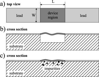
Figure 1: The schematic sketch presenting the structure under consideration: (a) top view of the device region (dark gray area) attached to the semi-infinite graphene leads (light gray areas), (b) free standing, rippled graphene layer, (c) graphene layer supported on the substrate (white area) in the presence of charged impurities (dots).

II.1 Basics

In order to describe transport and electronic properties of graphene we use the standard $p$-orbital tight-binding Hamiltonian,

$$H=\sum_{i}V_{i}\left|i\right\rangle\left\langle i\right|-\sum_{i,j}t_{i,j}\left|i\right\rangle\left\langle j\right|$$ (1)

limited to the nearest-neighbor hopping. $V_{i}$ denotes the external potential at the site $i$; the summation of $i$ runs over the entire lattice, while $j$ is restricted to the sites next to $i$. We related the spatial variation of the hopping integral $t_{i,j}$ with bending and stretching of the graphene layer due to warping as described in the next section.

The conductance $G$ and the electron density $n$ are computed with the aid of recursive Green function technique Zozoulenko1996 ; Zozoulenko2008 . We assume that the semi-infinite leads are perfect graphene ribbons, and the device region is a rectangular graphene strip and the imperfection (warping and long-range impurity potential) are restricted only to this area (see Fig.1). The zero-temperature conductance $G$ is given by the Landauer formula

$$G=\frac{2e^{2}}{h}T,$$ (2)

where $T$ is the total transmission coefficient between the leads. Then we calculated the conductivity

$$\sigma=\frac{L}{W}G,$$ (3)

the electron density

$$n(E)=\int_{0}^{E}dE\;\mathrm{DOS}(E),$$ (4)

and the mobility

$$\mu=\frac{\sigma}{en},$$ (5)

as a functions of the Fermi energy $E$ ($W$ and $L$ denote width and length of device, respectively). The density of states (DOS) was computed by averaging the local density of states (LDOS) over the whole device area. The LDOS is given by the diagonal elements of the total Green’s function.Zozoulenko2008

All the results presented here correspond to the ribbons of the zigzag orientation. Previous studies do not show a difference of the transport properties of the zigzag and armchair ribbons in the presence of disorder (provided the disorder concentration is sufficiently high).Martin ; Xu_bilayer We therefore expect that all the results reported here remain valid for the case of the armchair orientation as well.

The effect of warping is included in our model by modification of hopping integrals $t$ resulting from stretching (contraction) and $\pi-\sigma$ rehybridisation. The external potential of remote impurities (with inclusion the effect of screening by carries) is reflected in the model by changing of site energies. In the next subsection we present a detailed description of models for the warping and remote impurities.

II.2 Corrugation

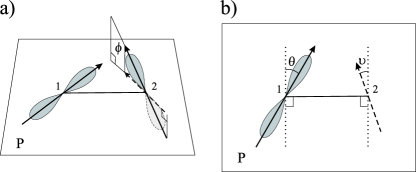
Figure 2: Definition of angles (used in Eq.(6)) describing alignment of $p$-orbitals of neighboring atoms. (a) $\phi$ denotes the angle between direction of orbital 2 and its projection (dashed arrow) on the plane $P$ spanned on the direction of the orbital 1 and the vector linking the centers of the orbitals 1 and 2; (b) Top view of the plane $P$. All vectors depicted here belong to the plane $P$ and have the same meaning as in (a). Dotted lines are perpendicular to the vector linking centers of the orbitals 1 and 2. Note that in the panel (b) the orbital 2 is not shown.

The mechanical properties of graphene can be modelled by treating this system as an elastic membrane. One can distinguish two modes of deformation: stretching/contraction and bending. Both of them affect the strength of carbon-carbon (C-C) bonds within the graphene sheet by changing the distance between carbon atoms and the alignment of their $p$-orbitals, respectively. In the tight-binding model the hopping integral corresponding the hybridised $\sigma-\pi$ bond is given by,Hansson-Stafstrom ; Mulliken

$$t(a,\theta,\phi,\vartheta) = \cos(\vartheta)\cos(\theta)\cos(\phi)t_{2p\pi,2p\pi}(a)$$

$$-\sin(\vartheta)\sin(\theta)t_{2p\sigma,2p\sigma}(a),$$

$$t_{2p\pi,2p\pi}(a) = \alpha_{\pi}e^{a\zeta}(1+a\zeta+\tfrac{2}{5}(r\zeta)^{2}+\tfrac{1}{15}(r\zeta)^{3}),$$

$$t_{2p\sigma,2p\sigma}(a) = \alpha_{\sigma}e^{a\zeta}(-1-a\zeta-\tfrac{1}{5}(a\zeta)^{2}+\tfrac{2}{15}(a\zeta)^{3}),$$ (6)

where $\alpha_{\pi}/t_{0}\approx-4.23$, $\alpha_{\sigma}/t_{0}\approx-4.33$ and $\zeta\approx 3.07$Å^-1 ($t_{0}=t(a_{0},0,0,0)=2.7$ eV and $a_{0}=1.42$ Å are the hopping integral and the C-C bond length for flat and unstained graphene ribbon, respectively). $t_{2p\pi,2p\pi}$ and $t_{2p\sigma,2p\sigma}$ denote the hopping integrals for pure $\pi$-bonds (in flat graphene) and $\sigma$-bonds (for collinear p-orbitals). The spatial orientation of the $p$-orbitals is described by the angles $\theta,\phi,\vartheta$ as presented in Fig.2.

The analysis of diffraction patterns of corrugated grapheneMeyer provides information about the range in which the normal to the surface varies. The measured range $\pm 5^{o}$ allows to estimate from Eq.(6) an impact of bending on the relative change of the hopping integral, $t(a_{0},\theta,\phi,\vartheta)-t_{0})/t_{0}\approx 0.4\%$. The information about the distribution of bond lengths in corrugated graphene is provided by the Monte Carlo simulations.Fasolino Using this data we can calculate the change of hopping integrals (6). The relative change $(t(a,0,0,0)-t_{0})/t_{0}$ for C-C bond variation $\Delta a=a-a_{0}$, corresponding to the half width at half height (HWHH) of the bond length distribution Fasolino , is approximately $2\%$. This comparison shows that the effect of strain (leading to a change of the bond length $\Delta a$) has a stronger impact on the modification of the hopping integrals in comparison to the effect of bending (related to the orbital alignment).

In a corrugated free standing membrane the bending and the in-plain strain are related to each other.Landau ; Nelson ; Witten For example, in order to produce a local minimum/maximum or a saddle-like area in a flat membrane it is necessary to introduce a strain (see Fig.3). Bending and strain of the free standing membrane can be related to the Gauss curvature:

$$c_{G}(x,y)=c_{1}(x,y)c_{2}(x,y),$$ (7)

which is the product of the minimum $c_{1}$ and maximum $c_{2}$ of normal curvaturesOprea (called by principal curvatures). The curvatures $c_{1}$, $c_{2}$ are given by the inverse radiuses of the local curvatures, $|c_{1}|=1/R_{1}$, $|c_{2}|=1/R_{2}$, see Fig.3. The sign of $c_{1}$ and $c_{2}$ depends on whether an intersection of normal plane with the surface is convex or concave. The positive value of $c_{G}$ at some point corresponds to the presence of a local minimum/maximun which requires streching of this region. For a saddle-like area (and negative value of $c_{G}$) the local contraction of a flat membrane is needed. The only kind of bending which does not produce a strain corresponds to developable surfaces (i.e. surfaces with zero Gauss curvature) such as e.g. a cylindrical tube, see Fig.3 (a).

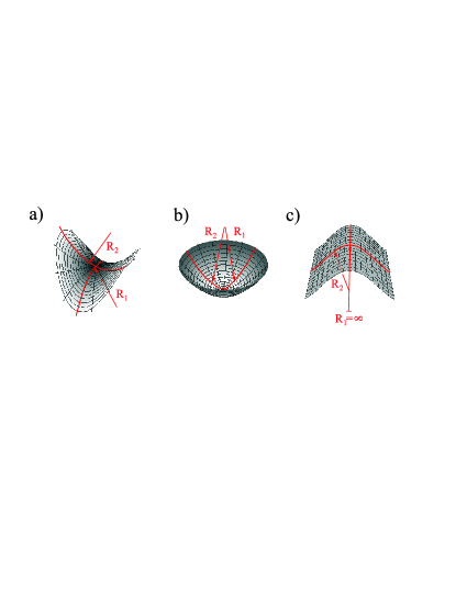
Figure 3: (color online) (a) A saddle-like surface and (b) a local minimum created by a nonuniform contraction (dark areas) and inflation (light areas) of a flat region. (c) developable surface (i.e. the surface with zero Gauss curvature). Each red curve and the vectors showing the radius of curvature lie in the same normal plane.

Because of a small variation of the relative change of the bond length $\Delta a/a_{0}$ we assume a linear dependence of the bond elongation/contraction $\Delta a$ on the Gauss curvature:

$$\Delta a(x,y)=kc_{G}(x,y).$$ (8)

The value of the coefficient $k$ was chosen to reproduce the range of $\Delta a$ variation computed in Fasolino . We estimated the HWHH of $\Delta a$ from the the C-C bond length distribution presented in Fasolino . Then, we computed the HWHH of $c_{G}$ distribution for a large (generated as described below) corrugated ribbon. The coefficient $k$ was defined as a ratio of the HWHHs for the $\Delta a$ and $c_{G}$ distributions.

In our model we do not take into account an influence of the surface corrugation on the position of carbon atoms. The positions of the centres of C-C bonds in flat lattice were projected onto a corrugated continuous surface. In these points the Gauss curvature was computed. The value of $c_{G}$ was used to calculate the change of the bond lengths (8). The angles $\theta,\phi,\vartheta$ (see Fig.2) were calculated from the alignment of normals representing the $\pi$ orbitals. The normals were computed at the ends of the projected bonds. The computed angles $\theta,\phi,\vartheta$ and C-C bond lengths $a=a_{0}+\Delta a$ were used to calculate the next-neighbor hopping integrals (6) in the corrugated ribbon.

In order to model the geometry of a corrugated ribbon we used the description of fluctuations of elastic membranes presented inFasolino . The ripples on the graphene surface can be expanded as a Fourier series of plane waves characterized by the wave vectors ${\bm{q}}$. In the harmonic approximationFasolino the in-plane- and out-of-plane displacement $h$ are decoupled. In this approximation the mean-square amplitude of Fourier component $h_{q}$ is given byNelson ; Katsnelson :

$$\left\langle h_{q}^{2}\right\rangle\sim\frac{1}{q^{4}}.$$ (9)

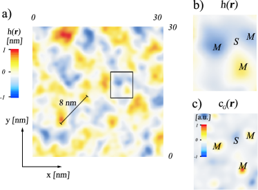
Figure 4: (color online) The model of ripples on the graphene surface. The black lines denote characteristic length of ripples 8nm ; (b) the magnified small area marked in (a) by a black frame; M and S stand for local maxima (minima) and saddle points, respectively; (c) the Gauss curvature corresponding to a part of the surface presented in (b) - red/orange (blue) areas mark regions with positive (negative) Gauss curvature.

It can be shown that the mean-square of the out-of-plane displacement $h$ scales quadratically with the linear size of the sampleFasolino :

$$\left\langle h^{2}\right\rangle=\sum_{q}\left\langle h_{q}^{2}\right\rangle\sim L^{2}.$$ (10)

According to Eq.(10) the height of the ripples increases quadratically with the sample size. It means that a large sample should be crumpled ($\left\langle h^{2}\right\rangle\gtrsim L$) which contradicts the experiments. The results consistent with the experiments where large sample remains approximately flat, are reproduced by the Monte Carlo simulationsFasolino where the dependence $\left\langle h_{q}^{2}\right\rangle\sim q^{-4}$ (Eq. (9)) remains valid for short wavelengths only, and saturates for the long wavelengths $\lambda=2\pi/q\gtrsim\lambda^{\ast}\approx 8$ nm. This mechanism is responsible for the existence of ripples of characteristic size $\sim\lambda^{\ast}$, see Fig. 4.

Using this guidance we modeled the corrugated surface in the following way. The surface $h({\bm{r}})$ was generated by a superposition of plane waves,

$$h({\bm{r}})=C\sum_{i}C_{q_{i}}\sin({\bm{q}}_{i}\cdot{\bm{r}}+\delta_{i}),$$ (11)

where ${\bm{r}}=(x_{1},x_{2})$ is the in-plane position vector. The directions $\varphi_{i}$ of the wave vectors ${\bm{q}}_{i}=q_{i}(\cos(\varphi_{i}),\sin(\varphi_{i}))$ and the phases $\delta_{i}$ were chosen randomly. The length of wave vectors $q_{i}$ covers equidistantly the range $2\pi/L<q_{i}<2\pi/(3a_{0})$, where $L$ is a leading linear size of the rectangular area and $a_{0}$ denotes the C-C bond length (we assume that $L\gg\lambda^{\ast}$). The amplitude of the mode was given by the harmonic approximation (9) $C_{q}=\sqrt{2\left\langle h_{q}^{2}\right\rangle}$ for the wave length $\lambda<\lambda^{\ast},$ otherwise it was kept constant and equal to $C_{q^{\ast}}$, where $q^{\ast}=2\pi/\lambda^{\ast}$. We introduced the normalisation constant $C$ to keep the averaged amplitude of the out-of-plane displacement $\bar{h}=\sqrt{2\left\langle h^{2}\right\rangle}$ equal to the experimental values $\bar{h}\approx 1$ nm for typical sizes of samples.

In Fig. 4 the graphene surface, generated by using the procedure described above, is shown. Long-wave ripples of the size $\sim\lambda^{\ast}\approx 8$ nm discussed above are clearly seen. A small area marked in a box in Fig. 4a is enlarged in Fig. 4b. In this region two minima (blue spots), one maximum (yellow spot) and one saddle region (white area between color spots) are shown. The relation between the geometry of the surface and its Gauss curvature can be visible in Fig. 4c. The regions of stretching (red and yellow spots) and contraction (blue spot) in Fig.4c correspond to the position of minima/maximum ($M$) and saddle area ($S$) in Fig.4b, respectively.

II.3 Long-range potential

The simplest model of charged impurities corresponds to the short-range $\delta$-function scattering centres,

$$V_{i}=U_{\delta}\sum_{i^{\prime}=1}^{N_{imp}}\delta\left({\bm{r}}_{i}-{\bm{r}}_{i^{\prime}}\right),$$ (12)

where $U_{\delta}$ is the strength of the individual scatterer, and the summation over $i^{\prime}$ runs over all impurities $N_{imp}$ in the device region. According to the Boltzmann transport theory the conductivity is $\sigma=(e^{2}/h)(2E\tau/\hbar)$, where $\tau$ stands for the scattering time. For the short range potential (12) the scattering time $\tau\sim 1/(E_{F}n_{imp}U_{\delta}^{2})$ (where $n_{imp}$ is the impurity concentration).ando In this model the calculated conductivity is independent on the electron density $n,$ whereas the mobility $\mu\sim 1/n$,Nomura2007 which contradicts the experimental observations.Bolotin This indicates that such a simplified model might not be appropriate for a description of a realistic system.

A long-range character of the electrostatic interaction is included in the model of bare Coulomb-like scattering centers,

$$V_{i}=\frac{1}{4\pi\epsilon_{r}\epsilon_{0}}\sum_{i^{\prime}=1}^{N_{imp}}\frac{e^{2}}{\left|{\bm{r}}_{i}-{\bm{r}}_{i^{\prime}}\right|},$$ (13)

where $\epsilon_{0}$ and $\epsilon_{r}$ stand respectively for the vacuum and relative permittivities. For this potential the conductivity is proportional to electron density, $\sigma\sim n/n_{imp}.$Nomura2007 . However, the application of the bare Coulomb potential can be justified only for low values of the electron density when the screening effects limiting the range of the potential are negligible.

The simplest screened potential is given by the Thomas-Fermi approximation,Adam2008

$$V_{i}=U_{TF}\sum_{i^{\prime}=1}^{N_{imp}}\frac{\exp\left(-\xi_{TF}|{\bm{r}}-{\bm{r}}_{i}|\right)}{\left|{\bm{r}}_{i}-{\bm{r}}_{i^{\prime}}\right|},$$ (14)

where the parameters $U_{TF}$ and $\xi_{TF}$ describe the strength and the range of the scattering centres for the Thomas-Fermi potential. The inclusion of screening allows to achieve both the limits of Coulomb scattering (for low $n$) and short-range scattering (for high $n$).

The singularity at ${\bm{r}}_{i}={\bm{r}}_{i^{\prime}}$ in the Thomas-Fermi potential (14) can cause numerical difficulties. In our calculation we utilize a model for screened scattering centers of the Gaussian shape commonly used in the literature where the potential on the site $i$ readsBardarson ; Rycerz ; Lewenkopf ,

$$V_{i}=\sum_{i^{\prime}=1}^{N_{imp}}U_{i^{\prime}}\exp\left(-\frac{|{\bm{r}_{i}}-{\bm{r}}_{i^{\prime}}|^{2}}{2\xi^{2}}\right),$$ (15)

where the height of scattering centers is uniformly distributed in the range

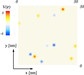
Figure 5: (color online) Illustration of the long-range potential, Eq.(15). The screening range is $\xi=4a_{0}$, the impurity concentration is $n_{imp}=10^{12}\,$cm^-2.

$U_{i^{\prime}}\in[-\delta,\delta]$. The strength and correlation between the scattering centers is described by the dimensionless correlator $K$,Rycerz ; Lewenkopf

$$\left\langle V_{i}V_{j}\right\rangle=\frac{K(\hbar v_{F})^{2}}{2\pi\xi^{2}}\exp\left(-\frac{|{\bm{r}_{i}}-{\bm{r}}_{j}|^{2}}{2\xi^{2}}\right),$$ (16)

(note that $\left\langle V_{i}\right\rangle=0$). The averaging is preformed for all possible configurations of system which differ only in the distribution of the position of the impurities ${\bm{r}}_{i^{\prime}}$ and the strength $U_{i^{\prime}}$ ($\delta$, $\xi$, $n_{imp}$ are kept constant).

For this impurity potential both the screening range $\xi$ and the impurity strength $\delta$ are independent on the electron density and play the role of parameters. They are related to $K$ by following formulaRycerz :

$$K\approx 40.5\tilde{n}_{imp}(\delta/t)^{2}(\xi/a_{0}),$$ (17)

where $\tilde{n}_{imp}=N_{imp}/N$ denotes the relative concentration expressed via the total number of impurities $N_{imp}$ and the atomic sites $N$ in a sample. In our calculation we use $n_{imp}=10^{12}$ cm^-2 as a typical value given in the experimentDu . We assumed that the screening range $\xi=4a_{0}$. The strength of impurities was chosen in order to get typical values of correlatorHwang2007 ; Bardarson (we chose $K=1,2,4,8$).

III Results and discussion

Let us start with the comparison of the effects of warping and charged impurities on the conductance of a graphene ribbon. Figure 6 shows the calculated conductance of a representative ribbon of the dimension $\sim 31\times 32$ nm. The warping modifies the conductance only slightly. For low energies close to the charge neutrality point the conductance steps remain practically unaffected. For higher energies the conductance steps become somehow distorted with the conductance plateaus being gradually shifted down and sharp minima appearing next to the rising edges of the plateaus. At the same time, in the presence of charged impurities even of a moderate strength the conductance of the ribbon is distorted substantially. The conductance steps are significantly washed out and the overall slope of the curve is lowered. Note that Fig. 6 shows the conductance of the ribbon for two representative impurity configurations with $n_{imp}=10^{12}$ and $4\times 10^{12}$ cm^-2 (dashed and dotted lines respectively). For higher energies (outside the first conductance step) the conductance for both cases shows rather similar features. However, for the energies corresponding to the the first conductance plateau the conductance of the sample with $n_{imp}=10^{12}$ cm^-2 (in contrast to the case of $n_{imp}=$ $4\times 10^{12}$ cm${}^{-2})$ remains practically unaffected. This is due to the fact that in the zigzag ribbons the transport in the vicinity of the charge neutrality point takes place via edge states strongly localized near the ribbon’s boundaries. For the considered impurity configuration for $n_{imp}=10^{12}$ cm^-2 no individual impurities are located close to the boundaries, and, as a result, the first conductance step remains practically unaffected.

Our results demonstrate that the modification of the nearest-neighbor hopping integrals $t$ resulting from stretching (contraction) and $\pi-\sigma$ rehybridisation has a little effect on the conductance in comparison to the effect of impurities. It should be also noted that the effect of the modification of the next-to-nearest hopping integrals $t^{\prime}$ is also weak in comparison to a realistic impurity potential. For example, Kim and Castro NetoKim_Castro_Neto estimated that the variation of the effective electrochemical potential generated by a spatial variation of $t^{\prime}$ is of the order of 30 meV, which is an order of magnitude smaller than a corresponding variation of the impurity potentialLewenkopf ; Ando . Hence, in our further analysis of the conductivity and the mobility of graphene ribbons we will take into to account the impact of charged impurities only.

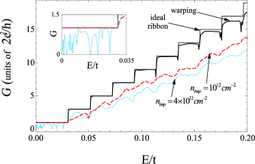
Figure 6: (color online) Effect of warping and charged impurities on the conductance of graphene nanoribbon of length $L=30.6$ nm and width $W=31.8$ nm ($250\times 150$ sites). The thin line shows the conductance steps for an ideal ribbon. The bold line denotes the conductance for a system with warping only; dashed and dotted lines refer to the conductance of a ribbon with impurities (without warping) with the concentration $n_{imp}=10^{12}\,$cm^-2 and $4\times 10^{12}$cm^-2 respectively. The strength of the impurities is $\xi=4a$, $K=2$. The inset shows an enhanced view of the conductance in the vicinity of the first conductance step.

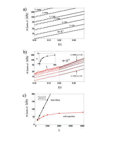
Figure 7: (color online) (a) The conductivity of (a) ideal ballistic nanoribbons and (b) nanoribbons with impurities as a function of the Fermi energy $E$. The nanoribbon lengths are $L=31,61,123,184,369,738$ nm corresponding to 250,500,1000,1500,3000,6000 sites. The conductivities in (b) are averaged over 10 impurities configuration. The dashed lines show the fit $\sigma\sim E^{\alpha}$ for the energies $E>0.2t$ as indicated by a vertical dotted line. (Here and hereafter we choose $E>0.2t$ because for lower energies the fitted dependencies deviate from the power-low behavior due to sample-specific fluctuations). The inset shows a dependence $\alpha=\alpha(L)$. The impurity parameters are $n_{imp}=10^{12}cm^{-2}$, $K=2$, $\xi=4a$. (c) The conductivity as a function of the ribbon length $L$ for ballistic ribbons and ribbons with impurities. The ribbon width is $W=53.1$ nm (250 sites).

Figure 8: (color online) (a) The DOS as a function of the Fermi energy of an ideal ribbon (solid line) and of a ribbon of the length $L=184$ nm (1500 sites) for a representative impurity configuration. (b) The dependence of the electron density $n$ on the Fermi energy for an ideal ribbon and for ribbons of various length with impurities. The parameters of the ribbons and the impurity strength are the same as in Fig. 7. (Note that the electron densities for the ribbons with the length $L>250$ sites are almost indistinguishable).

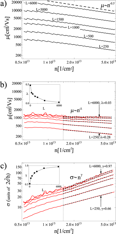
Figure 9: (color online) The mobility as a function of the electron density for (a) prefect zigzag nanoribbons and for (b) zigzag nanoribbons ribbon in the presence of charged impurities. The inset in (b) shows a dependence $\lambda=\lambda(L)$. (c) The conductivity a function of the electron concentration for nanoribbons in the presence of charged impurities. The inset in (c) shows a dependence $\gamma=\gamma(L)$. The parameters of the ribbons and the impurity strength are the same as in Figs. 7, 8. The dashed lines in (b) and (c) show the fits $\mu\sim\mu^{\lambda}$ and $\sigma\sim\sigma^{\gamma}$ for the electron densities $n\gtrsim 1.5\times 10^{13}$ cm^-2 (as indicated by a vertical dotted line). The mobilities and conductivities are averaged over 10 impurity configurations.

Let us now turn to the investigation of transition from the ballistic to diffusive regime of transport taking place as the size of the system increases. Because of computational limitations we keep in our study the width of the ribbon $W$ constant and increase its length $L,$ such that the diffusive regime is achieved when $L/W\gg 1$. We however expect that the results and conclusions presented in this paper would remain valid even for bulk diffusive samples with $L/W\sim 1.$

Figure 7 shows the conductivity $\sigma$ of ideal ballistic graphene ribbons of different lengths $L$ exhibiting a linear dependence on the electron energy $E$. This behavior of the conductivity reflects the corresponding linear dependence of the conductance $G$ of zigzag ribbons as a function of energy (see Appendix for details). Note that the conductance of an ideal ribbon in the ballistic regime is independent on the length of the system. Therefore, for fixed energy, the conductivity $\sigma=\frac{L}{W}G$ increases linearly with the ribbon length $L$ as illustrated in Fig. 7 (c). Apparently, in the ballistic regime, the conductivity does not exist as a local property and can not be considered as material parameter because it is size-dependent.

The conductivity of the ribbons of different lengths as a function of the electron energy in the presence of impurities is shown in Fig. 7 (b). The conductivity is strongly reduced in comparison to the ideal conductance steps and is no longer a linear function of the electron energy. Instead, it follows a power-law dependence

$$\sigma\sim E^{\alpha},$$ (18)

where the exponent $\alpha$ approaches $\alpha=2$ for sufficiently long ribbons (see inset to Fig. 7 (b)). Figure 7 (c) shows the dependence of the conductivity $\sigma$ on the length of the system in the presence of impurities. This dependence exhibits a clear saturation of the conductivity for sufficiently large systems, $L\gtrsim 6000$ sites (740 nm). In order to understand these features, in particular, the dependence of the conductivity on the system size $L,$ let us recall that the conductance of a disordered system is expected to obey the scaling law

$$\ln(1+1/g)=L/\xi_{loc},$$ (19)

where $\xi_{loc}$ is the localization length and $g=G/G_{0}$ is the dimensionless conductance ($G_{0}=2e^{2}/h$ being the conductance unit) Anderson . In this study we focus on the transport regime with many transmitted channels $g\gg 1.$ It follows from Eq. (19) that this corresponds to the case $\xi_{loc}\gg L,$ i.e. the localization length exceeds the size of the system and the conductance is inversely proportional to the length, $G\sim G_{0}/L.$ In this transport regime referred to as a diffusive (or Ohmic), the conductivity $\sigma$ is therefore independent on the system size and can be regarded as a local quantity. According to Fig. 7 (c) this transport regime is achieved for sufficiently long ribbons, $L\gtrsim 6000$ sites (740 nm). For smaller $L$ the system is in a quasi-ballistic regime when the conductivity $\sigma$ depends on the size of the system. In this case the conductance $G$ is apparently more appropriate quantity to describe the transport properties of the system at hand.

Let us now turn to the analysis of the mobility of graphene ribbons $\mu$. For a classical (Ohmic) conductor the mobility is the fundamental material property independent on the system size and the electron density. In contrast, for ballistic ribbons the mobility is size-dependent and decreases with increase of the electron density as $\mu\sim n^{-0.5}$ (see Appendix). Therefore one can expect that the mobility of ribbons varies as

$$\mu(n)\sim n^{-\lambda},$$ (20)

where the exponent $\lambda$ ranges from $0$ in the diffusive limit to $0.5$ in the ballistic limit.

In order to calculate the electron mobility $\mu=\sigma/en$ we, in addition to the conductivity $\sigma$, have to calculate the electron density $n$ in the ribbons (note that this step represents the most time-consuming part of our numerical calculations because in order to calculate $n$ we have to compute the DOS for all energies $0<E<E_{F}$). Figure 8 shows the DOS for a representative impurity configuration and electron densities for ribbons of different lengths calculated from the DOS according to Eq. (4). For ideal ribbons, the DOS follows an overall linear dependence on the energy with the singularities corresponding to openings of new propagating channels characteristic for quasi-1D systems. Because of this linear increase of the DOS, the electron density for an ideal ribbon follows a quadratic dependence on the energy, $n\sim E^{2}$ (see Appendix). Figure 8 (a) shows that the impurities only smear out the singularities in the DOS of an ideal ribbon, but do not reduce the DOS. Therefore, regardless of the ribbon lengths the average electron density in the ribbons with impurities is not reduced in comparison to the ideal ribbons, and follows the same quadratic dependence $n\sim E^{2}.$ This behavior is expected for the transport regime at hand when the localization length exceeds the size of the system, $\xi_{loc}\gg L,$ such that the averaged local DOS is essentially independent of the size of the system. Note that in the opposite regime of the strong localization, $\xi_{loc}\ll L,$ the electron density in ribbons is strongly reduced due to the effect of impurities.Xu_bilayer .

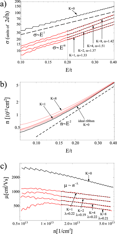
Figure 10: (color online) (a) The conductivity and (b) the electron density versus the Fermi energy and (c) the mobility versus the electron density for graphene nanoribbon for different impurity strengths $K=1,2,4,8$; $\xi=4a$, $n_{imp}=10^{12}\,$cm^-2. The ribbon’s dimension is $L\times W=123\times 53$ nm${}^{2}(1000\times 250$ sites). The dashed lines in (a) and (c) show the fits according to Eqs. (18) and (19) for respectively $E>0.2t$ and $n\gtrsim 1.5\times 10^{13}$ cm^-2. (The start of respective fitting intervals are indicated by vertical dotted lines).

For low energies close to the charge neutrality point $E=0$ the DOS of the system with impurities shows sharps peaks whose positions are strongly system-dependent, see Fig. 8 (a). This is because in this energy interval the system is in the strong localization regime with the localization length being smaller than the system size (for an analysis of this transport regime see Ref. Xu_bilayer, ). In this energy interval the DOS is strongly system-dependent because it reflects a particular configuration of the impurity potential. This explains some differences in the electron densities for different ribbons in Fig. 8 (b) (especially for the shortest one with $L=250$ sites), because the integration in Eq. (4) includes all the energies (below Fermi energy), including those close to $E=0$ where the DOS can show strong system-specific fluctuations.

Having calculated the electron density and the conductivity, we are in a position to discuss the mobility of the system at hand. The mobility of the ideal ribbons of different lengths $L$ as a function of the electron density is shown in Fig. 9 (a). This corresponds to the ballistic regime with $\lambda=0.5$. For a given electron density the mobility of the ballistic ribbons is proportional to the ribbon length, $\mu\sim L$ (because $\mu=\sigma/en$ and $\sigma\sim L,$ see Fig. 7 (c)).

Let us now investigate how the mobility of a ribbon evolves as we go from the quasi-ballistic to the diffusive regime by increasing the system size. Figure 9 (b) shows the mobility of the ribbon with impurities as a function of the electron density. As expected, this dependence satisfies Eq. (20). The dependence $\lambda=\lambda(L)$ is shown in the inset to Fig. 9 (b). This dependence clearly demonstrates that we approach the diffusive regime (with the expected value of $\lambda=0)$ as the length of the ribbons becomes sufficiently long ($L\gtrsim 740$ nm). This is fully consistent with the behavior of the conductivity discussed above which exhibits a transition to the diffusive transport regime as the length of the ribbon increases.

The calculated dependence $\lambda=\lambda(L)$ is also consistent with the energy dependence of the conductivity which approaches the quadratic behavior $\sigma\sim E^{2}$ in the diffusive regime (see inset to Fig. 7 (b)). Because $n\sim$ $E^{2}$ regardless of the regime (ballistic, quasi-ballistic, or diffusive), the mobility $\mu=\sigma/en$ becomes independent on the energy (and thus on the electron density with $\lambda=0$) only when $\sigma\sim E^{2}.$ To illustrate this we in Fig. 9 (c) present the dependence $\sigma=\sigma(n)$ which is plotted by combining previously calculated dependencies $\sigma=\sigma(E)$ and $n=n(E).$ As expected from Eqs. (5) and (20) it follow a dependence

$$\sigma(n)\sim n^{\gamma},$$ (21)

where the exponent $\gamma$ ranges from $1$ in the diffusive limit to $0.5$ in the ballistic limit.

All the results for the conductivity, electron density and the mobility in the graphene ribbons presented above correspond to the case of one representative impurity strength $n_{imp}=10^{12}$cm^-2, $K=2$, $\xi=4a$. It is important to stress that the scaling laws discussed above are rather insensitive to a particular realization of the potential configuration or the impurity strength provided that the system is in the transport regime when the localization length is larger than the ribbon size. This is illustrated in Fig. 10 showing the conductivity, the electron density and the mobility in graphene ribbons for different impurity strength $K=1,2,4,8$. As expected, the electron density is similar for all ribbons, especially for high energies, see Fig. 10 (b). When the impurity strength increases the conductivity apparently decreases, see Fig. 10 (a). This decrease of the conductivity leads also to the decrease of the mobility as shown in Fig. 10 (c). However, the exponents in the scaling laws (18) and (19) are not particularly sensitive to the variation of the impurity strength $K.$ A small difference in scaling exponents for different impurity strengths has a statistical origin and this difference diminishes as a number of impurity configurations used in calculations of each curve is increased.

Let us now use our results to discuss available experimental data. In experiments, the electron density dependence of the mobility, $\mu=\mu(n)$, and the conductivity, $\sigma=\sigma(n)$, are accessible Bolotin ; Du . The dependencies (20), (21) can therefore be used to extract information about the transport regime for the system at hand. For example, for the mobility the exponent $\lambda=0.5$ would correspond to a purely ballistic transport regime, whereas $\lambda=0$ would describe a purely diffusive one. An intermediate exponent $0<\lambda<0.5$ would indicate the quasi-ballistic transport regime; the more close the value of $\lambda$ to $0$, the more diffusive the system is. Similar arguments applies to the conductivity where the corresponding exponent $\gamma$ lies between 0.5 and 1. For example, the mobility measured by Du et al. Du corresponds to $\lambda=0.5$ suggesting a purely ballistic transport regime. The electron density dependence of the mobility and conductivity in graphene ribbons was also studied by Bolotin et al.Bolotin The measured conductivity follows the sublinear behavior (21) with $\gamma<1$. They attributed the deviation from the linear dependence to the effect of the short-range scattering. Taking into account that the mean free path in their device is comparable to the device dimension, we can provide an alternative interpretation of their findings arguing that the observed in Bolotin sublinear behavior represents a strong evidence of the quasi-ballistic transport regime.

IV Conclusions

In the present study we perform numerical calculations of the conductance of graphene ribbons based on the Landauer formalism and the tight-binding p-orbital Hamiltonian including the effect of warping of graphene and realistic long-range impurity potential. The effect of warping is included in our model by modification of the nearest neighbor hopping integrals resulting from stretching/contraction of the surface and the $\pi-\sigma$ rehybridisation. We find that the modification of the next-neighbor hopping due to the warping of the graphene surface has a negligible effect on the conductance in comparison to the effect charged impurities even for moderate strength and concentration.

The main focus of our study is a transition from the ballistic to the diffusive transport regime in realistic graphene ribbons with long-range impurities which occurs as the size of the system increases. We keep in our study the width of the ribbon $W$ constant and increase the ribbon length $L,$ such that the diffusive regime is achieved when $L/W\gg 1$. We however expect that the results and conclusions presented in this paper would remain valid even for bulk diffusive samples with $L/W\sim 1,$ as soon as the localization length exceeds the size of the system.

We demonstrated that the conductivity of graphene ribbons follows a power-law dependence $\sigma\sim E^{\alpha}$ with $1\leq\alpha\lesssim 2.$ The case $\alpha=1$ corresponds to the ballistic regime whereas $\alpha=2$ corresponds to the diffusive regime which is reached for sufficiently long ribbons. In the ballistic regime the conductivity scales linearly with the length of the system $L$, whereas in the diffusive regime the conductivity saturates with $L$.

We find that the average electron density in the ribbons with impurities is practically not reduced in comparison to the ideal ribbons, and follows the same quadratic dependence $n\sim E^{2}$ regardless of the transport regime (ballistic, quasi-ballistic or diffusive). This behavior is consistent with the exponent $\alpha=2$ reached in the diffusive case, because in this case the mobility $\mu=\sigma/en$ becomes independent on the energy (and hence on the electron density) as expected for the diffusive regime.

In experiments the electron density dependence of the mobility, $\mu=\mu(n)$, is accessible. We find that the mobility of graphene ribbons varies as $\mu(n)\sim n^{-\lambda},$ with $0\leq\lambda\lesssim 0.5.$ The exponent $\lambda$ depends on the size of the system with $\lambda=0.5$ corresponding to short ribbons in the ballistic regime, whereas the diffusive regime $\lambda=0$ (when the mobility is independent on the electron density) is reached for sufficiently long ribbons. Our results can be used for the interpretation of the experimental data when the value of the parameter $\lambda$ can be used to distinguish the transport regime of the system (i.e. ballistic, quasi-ballistic or diffusive). The corresponding electron density dependence for the conductivity is, $\sigma(n)\sim n^{-\gamma},$where the exponent $\gamma$ ranges from $1$ in the diffusive limit to $0.5$ in the ballistic limit. Based on our findings we discuss the available experiments and provide an alternative interpretation of some experimental conclusions.Bolotin ; Du

Our calculations also demonstrate that in the quasi-ballistic regime (which corresponds to many experimental studies) the mobility and the conductivity of the structure at hand strongly depend on the system size. Therefore in this regime the conductivity does not exist as a local property and the mobility can not be considered as a well-defined material parameter because of its dependence on the system size.

Appendix A Electron conductivity, mobility and electron density in the ballistic regime

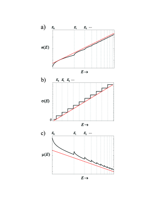
Figure 11: (Color online) (a) The electron density, (b) the conductivity (c) and the mobility as a functions of the Fermi energy for a zigzag nanoribbon. Red lines correspond to the approximate expressions (25), (27), (28), whereas the black lines to the exact expressions (22), (26).

In the low-energy limit close to the charge neutrality point $E=0$ the electron density of the zigzag graphene nanoribbon of the width $N$ reads,Shylau

$$n(E)=\frac{4}{\pi\sqrt{3}}\frac{1}{t_{0}a_{0}}\sqrt{E^{2}-E_{m}^{2}}\;\theta(|E|-|E_{m}|),$$ (22)

where the threshold energies have the form,

$$E_{m}=\frac{3\pi}{8}t_{0}a_{0}\frac{1}{W}(m+\tfrac{1}{2}),\;m=0,1,2,\ldots.$$ (23)

Noticing that the function $\sqrt{E^{2}-E_{m}^{2}}$ approaches $E$ for $E\gg E_{m}$ we can write the electron density in the approximate form:

$$n(E)\approx\frac{4}{\pi\sqrt{3}}\frac{1}{t_{0}a_{0}}E\sum_{m}\;\theta(|E|-|E_{m}|).$$ (24)

Summation of $\theta$-functions in Eq. (24) gives a number of propagating modes at the given energy. Expressing this number with energy by making use of Eq. (23) and approximating $E\approx E_{m}$ we obtain,

$$n(E)\approx\frac{32}{\pi^{2}3\sqrt{3}}\frac{1}{t_{0}^{2}a_{0}^{2}}WE^{2}.$$ (25)

A comparison of the approximate expression (25) with the exact one (22) is shown in Fig. 11(a).

In the low-energy limit close to the charge neutrality point $E=0$ the conductivity of the zigzag graphene nanoribbon of the width $N$ reads,onipko

$$\sigma(E)=\frac{2e^{2}}{h}\frac{L}{W}\left(\sum_{m}2\theta(|E|-|E_{m}|)-1\right).$$ (26)

Using similar approximations as above we obtain,

$$\sigma(E)\approx\frac{2e^{2}}{h}\frac{16}{3\pi}\frac{1}{t_{0}a_{0}}LE.$$ (27)

Finally, substituting Eq. (27) and (25) into the definition of the mobility we obtain,

$$\mu=\frac{\sigma}{en}\approx\frac{e}{h}\pi\sqrt{3}t_{0}a_{0}\frac{L}{W}E^{-1}=\frac{e}{h}\frac{4\sqrt{2}}{\sqrt[4]{3}}\frac{L}{\sqrt{W}}n^{-0.5}.$$ (28)

A comparison of the approximate expression for the conductivity and the mobility with the exact ones is shown in Fig. 11 (b), (c).

It should be noted that the expressions (22), (24), (25) for the electron density $n$ do not include a contribution from the edge states existing in the zigzag nanoribbons for the energies close to $E=0$. Because of this the electron density of the nanoribbon shown in Fig. 11 vanishes at $E=0$ and the mobility $\mu$ exhibits a singularity. Accounting for the contribution from the edge state in exact numerical calculations leads to the finite values of $n$ and $\mu$ at $E=0.$ However, for high energies sufficiently away the charge neutrality point this contribution does not practically affect $n$ and $\mu$, which justifies the utilization of expressions (22)-(28).

References

- (1) K. S. Novoselov, A. K. Geim, S. V. Morozov, D. Jiang, Y. Zhang, S. V. Dubonos, I. V. Grigorieva, and A. A. Firsov, Science 306, 666 (2004).
- (2) A. K. Geim and K. S. Novoselov, Nat. Mater. 6, 183 (2007); A. H. Castro Neto, F. Guinea, N. M. R. Peres, K. S. Novoselov and A. K. Geim, Rev. Mod. Phys. 81, 109 (2009).
- (3) T. Ando, J. Phys. Soc. Jpn. 75, 074716 (2006).
- (4) K. Nomura and A. H. MacDonald, Phys. Rev. Lett. 96, 256602 (2006).
- (5) S. Adam, E. H. Hwang, V. M. Galitski, and S. Das Sarma, PNAS 104, 18392 (2007).
- (6) E. H. Hwang, S. Adam, and S. Das Sarma, Phys. Rev. Lett. 98, 186806 (2007).
- (7) K. Nomura and A. H. MacDonald, Phys. Rev. Lett. 98, 076602 (2007).
- (8) K. I. Bolotin, K. J. Sikes, Z. Jiang, M. Klima, G. Fudenberg, J. Hone, P. Kim, H.L. Stormer, Solid State Comm. 146, 351 (2008).
- (9) Xu Du, I. Skachko, A. Barker and E. Y. Andrei, Nature Nanotech. 3, 491 (2008).
- (10) J. C. Meyer, A. K. Geim, M. I. Katsnelson, K. S. Novoselov, T. J. Booth and S. Roth, Nature 446, 60 (2007).
- (11) A. Fasolino, J. H. Los and M. I. Katsnelson, Nature Materials 6, 858 (2007).
- (12) Eun-Ah Kim and A. H. Castro Neto, Eur. Phys. Lett. 84, 57007 (2008).
- (13) M. I. Katsnelson and A. K. Geim, Phil. Trans. R. Soc. A 366, 195 (2007)
- (14) F. de Juan, A. Cortijo, and M. A. H. Vozmediano Phys. Rev. B 76, 165409 (2007).
- (15) A. Isacsson, L. M. Jonsson, J. M. Kinaret, and M. Jonson, Phys. Rev. B 77, 035423 (2008).
- (16) V. Geringer, M. Liebmann, T. Echtermeyer, S. Runte, M. Schmidt, R. Rückamp, M. C. Lemme, and M. Morgenstern, Phys. Rev. Lett. 102, 076102 (2009).
- (17) A. Deshpande, W. Bao, F. Miao, C. N. Lau, and B. J. LeRoy Phys. Rev. B 79, 205411 (2009).
- (18) J. Sabio, C. Seoánez, S. Fratini, F. Guinea, A. H. Castro Neto, and F. Sols, Phys. Rev. B 77, 195409 (2008).
- (19) F. Miao, S. Wijeratne, Y. Zhang, U. C. Coskun, W. Bao, and C. N. Lau, Science 317, 1530 (2007).
- (20) S. Russo, J. B. Oostinga, D. Wehenkel, H. B. Heersche, S. S. Sobhani, L. M. K. Vandersypen, and A. F. Morpurgo, Phys. Rev. B 77, 085413 (2008).
- (21) J. H. Bardarson, J. Tworzyłdo, P. W. Brouwer, and C. W. J. Beenakker, Phys. Rev. Lett. 99, 106801 (2007)
- (22) A. Rycerz, J. Tworzyłdo, and C. W. J. Beenakker, Eur. Phys. Lett. 79, 57003 (2007)
- (23) D. A. Areshkin, D. Gunlycke, and C. T. White, Nano. Lett. 7, 204 (2007).
- (24) E. Louis, J. A. Vergés, F. Guinea, and G. Chiappe, Phys. Rev. B 75, 085440 (2007).
- (25) D. Gunlycke, D. A. Areshkin, and C. T. White, Appl. Phys. Lett. 90, 142104 (2007).
- (26) T. C. Li and S.-P. Lu, Phys. Rev. B 77, 085408 (2008).
- (27) D. Querlioz, Y. Apertet, A. Valentin, K. Huet, A. Bournel, S. Galdin-Retailleau, and P. Dollfus, Appl. Phys. Lett. 92, 042108 (2008).
- (28) Y.-M. Lin, V. Perebeinos, Zh. Chen, and Ph. Avouris, Phys. Rev. B 78, 161409(R) (2008).
- (29) M. Evaldsson, I. V. Zozoulenko, Hengyi Xu and T. Heinzel, Phys. Rev. B 78, 161407(R) (2008)
- (30) C. H. Lewenkopf, E. R. Mucciolo, and A. H. Castro Neto, Phys. Rev. B 77, 081410(R) (2008)
- (31) E. R. Mucciolo, A. H. Castro Neto, and C. H. Lewenkopf, Phys. Rev. B 79, 075407 (2009).
- (32) H. Xu, T. Heinzel, and I. V. Zozoulenko , Phys. Rev. B 80, 045308 (2009).
- (33) E. Rossi and S. Das Sarma, Phys. Rev. Lett. 101, 166803 (2008)
- (34) Z. Chen, Y.-M. Lin, M. J. Rooks and P. Avouris, Physica E 40, 228 (2007).
- (35) M. Y. Han, B. Ozyilmaz, Y. Zhang, and P. Kim, Phys. Rev. Lett. 98, 206805 (2007).
- (36) I. V. Zozoulenko, F. A. Maao, and E. H. Hauge, Phys. Rev. B 53, 7975(1996)
- (37) H. Xu, T. Heinzel, M. Evaldsson and I. V. Zozoulenko, Phys. Rev. B 77, 245401 (2008)
- (38) A. Hansson and S. Stafström, Phys. Rev. B 67, 075406 (2003)
- (39) R. S. Mulliken, C. A. Rieke, D. Orloff, and H. Orloff, J. Chem. Phys. 17, 1248 (1949)
- (40) L. D. Landau, and E. M. Lifshitz, Theory of Elasticity 3rd Edition, (Pergamon, New York, 1986)
- (41) D. R. Nelson, T. Piran, and S. Weinberg (eds), Statistical Mechanics of Membranes and Surfaces (World Scientific, Singapore, 2004)
- (42) T. A. Witten, Rev. Mod. Phys. 79, 643 (2007)
- (43) J. Oprea, Differential Geometry and its Applications 2nd Edition, (Pearson Prentice Hall, Upper Saddle River, New Jersey, 2004)
- (44) N. H. Shonand, T. Ando, J. Phys. Soc. Jpn. 67, 2421 (1998)
- (45) S. Adam and S. Das Sarma, Phys. Rev. B 77, 115436 (2008)
- (46) P. W. Anderson, D. J. Thouless, E. Abrahams, and D. S. Fisher, Phys. Rev. B 22, 3519 (1980); P. A. Lee and T. V. Ramakrishnan, Rev. Mod. Phys. 57, 287 (1985).
- (47) A. A. Shylau, J. W. Klos, and I. V. Zozoulenko, arXiv:0907.1040v1 [cond-mat.mes-hall]
- (48) A. Onipko, Phys. Rev. B 78, 245412 (2008)