POLARIZATION OF BREMSSTRAHLUNG AT ELECTRON SCATTERING
IN ANISOTROPIC MEDIUM

Abstract

Bremsstrahlung from relativistic electrons is considered under conditions when some transverse direction of momentum transfer is statistically preferred. It is shown that in the dipole approximation all the medium anisotropy effects can be accumulated into a special modulus-bound transverse vector, $\bm{N}$. To exemplify a target with $N^{2}\sim 1$, we calculate radiation from electron incident at a small angle on an atomic row in oriented crystal. Radiation intensity and polarization dependence on the emission angle and frequency for constant $\bm{N}$ is investigated. Net polarization for the angle-integral cross-section is evaluated, which appears to be proportional to $N^{2}/2$, and decreases with the increase of the photon energy fraction. A prominent feature of the radiation angular distribution is the existence of an angle at which the radiation may be completely polarized, in spite of the target complete or partial isotropy – that owes to existence of an origin-centered tangential circle for polarization in the fully differential radiation probability kernel. Possibilities for utilizing various properties of the polarized bremsstrahlung flux for preparation of polarized photon beams and for probing intrinsic anisotropy of the medium are analyzed.

I Introduction

Relativistic electrons interacting with matter are efficient sources of gamma-radiation, which may be applied either for probing nuclei and hadrons Proc gamma-nucl , or to deliver information about the medium the electrons are passing through. The full set of the radiation characteristics includes photon polarization, which correlates with the preferential direction of acceleration of the radiating particle in the medium, as well as with the photon emission azimuthal angle. Detection techniques sensitive to $\gamma$-quantum polarization have been developed to date in a rather wide range of photon energies RHESSI ; nucl polarimeters ; pol-through-or-cryst .

For electron scattering on one atom, which is practically a spherically-symmetric object, the whole problem is axially symmetric, and thereby net polarization of the radiation (i. e., when integrated over the relativistically small emission angles) vanishes. In contrast, in condensed matter, particularly in crystals, due to correlation of atomic positions, the aggregate fields can be highly anisotropic. But in what concerns bremsstrahlung, it is essential to recall that the major contribution to the radiation intensity comes from spatial regions with highest electromagnetic field strength, whereas for atoms those regions are perinuclear and non-overlapping, containing centrally-symmetric fields, anyway. To compete with this contribution, soft action of the atoms on the radiating fast electron must be enhanced, in coherent manner. So far, examples of highly azimuthally anisotropic motion or scattering of electrons in crystals were basically restricted to (planar) channeling Gemmel-Kumakhov , and coherent bremsstrahlung Diambrini ; Ter-Mik . These cases demand perfect crystals, high initial electron beam collimation, and precise crystal orientation with respect to the incident beam. An extra benefit is the fair monochromaticity of the emitted $\gamma$-radiation.

But in case if one is interested in radiation polarization only, regardless of its monochromaticity, and so seeks only scattering azimuthal anisotropy, not periodicity of the electron motion in the medium, it seems sufficient to get by with a much rougher experimental setup. Taking a sufficiently thin crystal cut about perpendicularly to one of the main crystallographic directions, one can expect atomic chains along this direction to maintain their orientation within the crystal thickness. An elementary interaction of a fast charged particle with a string making a relatively small angle with the particle direction of motion already introduces an asymmetry between two transverse directions for particle deflection; the ordering of strings in transverse directions on the crystal area is not prerequisite.

The purpose of the present article is to calculate scattering azimuthal asymmetry and the bremsstrahlung polarization for the abovementioned physical problem of electron-string interaction, and estimate minimal conditions for the crystal quality and orientation, beam collimation degree, etc. Thereat, it may not suffice to deal with scattering on one string, since a statistical ensemble of strings contributes. Besides that, even for thin crystals the thickness may be large enough for failure of factorization between scattering and radiation, so that radiation and motion in the external field become an inseparable problem.

Concerning prospects of statistical and non-factorized description of the radiation spectral intensity, a simplifying property of electron propagation in atomic matter is that small (relative to the electron mass) momentum transfers to atoms dominate , justifying equivalent photon WW ; Bertulani ; Ter-Mik , also known as dipole approximation BKStrakh . The value of the latter approximation is that it makes the radiation differential probability simply a quadratic form in the transferred momentum. That permits statistical averaging over the momentum transfers in matter, basically, in a model-independent way. As we will show, all the anisotropy effects get absorbed into a single transverse vector, pointing along the preferential direction of momentum transfer in the medium, and having the absolute value related to the asymmetry degree. However, at a substantial non-factorizability of radiation and scattering, the magnitude of this vector can depend on the emitted photon energy.

The plan of the paper is as follows. In Sec. II we define the equivalent photon approximation for the bremsstrahlung process, for simplicity initially presuming the scattering factorization. We discuss the kinematical relations obeyed by the polarized photons. In Sec. III we turn to averaging over momentum transfers in matter which requires relaxing the scattering factorization assumption, and analyze possibilities for obtaining high azimuthal anisotropy with macroscopic targets. In Sec. IV we specialize to the problem of electron interaction with atomic strings, first evaluating bremsstrahlung one one string, and then estimating the effects of multiple scattering. In Sec. V we evaluate spectra and angular distributions for the polarization bremsstrahlung yield at an arbitrary, but (for simplicity) photon momentum independent, macroscopic anisotropy parameter. A summary is given in Sec. VI.

II Basic bremsstrahlung properties (factorization conditions)

The general statement of bremsstrahlung problem assumes a relativistic electron (mass $m$, initial 4-momentum $p=(E,\bm{p})$) scattering on a static solid target, not necessarily intrinsically isotropic, and detecting $\gamma$-quanta in the typical direction close to $\bm{p}$, hence most probably emitted by incident fast electrons, and most probably not more than one $\gamma$-quantum per electron. In a fully exclusive event, when the final electron has a well-defined 4-momentum, as well (denote it as $p^{\prime}=(E^{\prime},\bm{p}^{\prime})$), the 4-momentum conservation law and the mass shell conditions read :

$$p=p^{\prime}+k+q,$$

$$p^{2}=p^{\prime 2}=m^{2},\quad k^{2}=0,$$

where $k=(\omega,\bm{k})$ is the emitted $\gamma$-quantum momentum, and $q=(0,\bm{q})$ – the total momentum transferred from the electron to the target.

Polarizations of the photons exchanged with the target can be regarded as certain, described by a vector $e^{\mu}$, granted that the target is heavy and recoilless. To view it as a source of a static potential in the laboratory frame, we assume

$$e=(1,\bm{0})$$ (1)

or Lorentz invariantly,

$$e\cdot q=0,\qquad e^{2}=1.$$ (2)

The final photon polarization vector $e^{\prime\mu}$ in any gauge satisfies

$$e^{\prime}\cdot k=0,\qquad e^{\prime 2}=-1.$$

The natural gauge for the final real photon is, in the lab frame

$$e^{\prime}=\left(0,\bm{e}^{\prime}\right).$$

Initial and final electron bispinors $u$, $u^{\prime}$ obey Dirac equations

$$(p\cdot\gamma-m)u=0,\qquad\bar{u}^{\prime}(p^{\prime}\cdot\gamma-m)=0,$$ (3)

and the normalization conditions

$$\bar{u}u=\bar{u}^{\prime}u^{\prime}=2m.$$

Large 4-momenta $p$, $p^{\prime}$, $k$ in the lab frame are nearly collinear. Their spatial direction we will let to be $Oz$; spatial vector components orthogonal to $Oz$ with be marked with a subscript $\perp$. The naturally emerging ratios of the large collinear momenta will defined in terms of their energy components:

$$\frac{\omega}{E}=x_{\omega}\lesssim 1,\qquad\frac{E^{\prime}}{E}=1-x_{\omega}\sim 1.$$ (4)

II.1 Scattering factorization conditions

Let us begin with a simplified problem of radiation under the scattering factorization condition. The scattering factorization property implies finite-range interaction during an ultra-relativistic collision, when the time of the scattering is much shorter than the typical time of decay processes, including the radiation emission (a sort of impulse approximation). That makes the photon predominantly emitted from the electron ‘legs’ prior to and after the scattering. To remind how it formally manifests itself in different popular frameworks, first refer to the target rest frame, where one observes relativistic extension (by Lorentz-factor $\gamma$) of the radiation formation length Ter-Mik

$$l_{\mathrm{form}}=q_{z}^{-1}\sim\frac{\gamma(1-x_{\omega})}{x_{\omega}m}$$ (5)

($q_{z}$ stands for the longitudinal component of typical $q$ in the process, more precisely – see Eq. (24) below), relative to the field localization domain $\sim r_{\text{a}}$ (the atomic radius). Thus, the factorization condition is

$$r_{\text{a}}\ll l_{\mathrm{form}},\quad\mathrm{i.\,e.,}\quad q_{z}r_{\text{a}}\ll 1.$$ (6)

From another viewpoint, in a frame where the electron is non-ultra-relativistic and evolves together with its electromagnetic proper-field at times $\sim m^{-1}$, the target atom becomes longitudinally Lorentz-contracted to the size $\sim r_{\text{a}}/\gamma$, and appears to the radiating electron as a short kicker, leading again to same condition (6). Finally, when working in the momentum representation, say, in terms of Feynman diagrams, the emitted real photon typically changes the electron virtuality (square of its 4-momentum in a virtual state) by amount $\sim m^{2}$. As for momentum exchange with the target, individual longitudinal transfers $q_{z}^{(i)}$ which are of the order of $r_{\text{a}}^{-1}$ (though $\sum_{i}q_{z}^{(i)}=q_{z}$ is kinematically restricted to be $\ll r_{\text{a}}^{-1}$) make denominator of the electron’s propagator relativistically large – but a proper compensation arrives from the energy numerator, typical for vector coupling theories (the same reason as for finiteness of forward cross-sections – see, e. g., Cheng-Wu ). However, if the real photon is emitted in between the momentum exchanges with the target, it splits a hard electron propagator into two hard ones, without a numerator compensation. Therefore, largest are contributions from diagrams in which the real photon is the first or the last one in the sequence, leading to the same ordering of radiation and scattering as inferred from the previous spatial consideration – see Fig. 1. The technical profit from the encountered ordering is that it allows factorizing the amplitude of the entire process into a (nearly on-shell) amplitude of scattering and the amplitude of radiation at a single scattering act Olsen-Maximon-Wergeland .

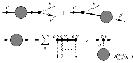
Figure 1: Factorization of the photon radiation amplitude at electron scattering on a static source of electric field. Line thickness reflects the electron virtuality, or fastness of the process: thinnest lines represent real electrons, medium thickness lines – propagation between the scattering and photon emission, thick line – propagation between the scatterings.

As for the Dirac matrix structure of the scattering amplitude, for small-angle scattering it is particularly simple. In each contribution to the amplitude from propagation between the scatterings (say, on the initial end)

$$e\cdot\gamma\frac{p\cdot\gamma-\sum q^{(i)}\cdot\gamma+m}{(p-\sum q^{(i)})^{2}-m^{2}}e\cdot\gamma,$$

the spin numerator can always be recast as

$$e\cdot\gamma\left(p\cdot\gamma-\sum q^{(i)}\cdot\gamma+m\right)e\cdot\gamma\qquad\qquad$$

$$=2e\cdot pe\cdot\gamma+\left(-p\cdot\gamma+\sum q^{(i)}\cdot\gamma+m\right)e^{2}.$$ (7)

With $e\cdot p/m=\gamma$ (Lorentz-factor), $\bar{u}^{\prime}e\cdot\gamma u/\bar{u}^{\prime}u\sim\gamma$, the second term in (7) is generally $\mathcal{O}\left(\gamma^{-2}\right)$ relative to the first one and can be neglected within the accuracy of the factorization approximation (6). Proceeding so in all orders, the matrix scattering amplitude can be written as $e\cdot\gamma A_{\text{scat}}^{\text{diffr}}(q_{\perp})$, where $A_{\text{scat}}^{\text{diffr}}(q_{\perp})$ is the spin-independent near-forward angle scattering amplitude including all orders in perturbation theory. Physically, it can be regarded as diffractive (potential, non-absorptive), whereby its spin independence looks intuitive.

Ultimately, the factorization theorem for the small-angle bremsstrahlung process assumes the form

$$T_{\text{fact}}=A^{\text{diffr}}_{\text{scat}}\left(q_{\perp}\right)\sqrt{4\pi}eM_{\text{rad}}\left(q_{\perp},k\right)\left\{1+\mathcal{O}\left(q_{z}r_{\text{a}}\right)\right\},$$ (8)

with

$$M_{\text{rad}}=\bar{u}^{\prime}\bigg{(}\frac{e^{\prime*}\cdot\gamma(p\cdot\gamma-q\cdot\gamma+m)e\cdot\gamma}{2p^{\prime}\cdot k}\qquad\quad$$

$$-\frac{e\cdot\gamma(p^{\prime}\cdot\gamma+q\cdot\gamma+m)e^{\prime*}\cdot\gamma}{2p\cdot k}\bigg{)}u,$$ (9)

the tree-level radiation matrix element, and $A^{\text{diffr}}_{\text{scat}}(q_{\perp})$ – the exact elastic scattering amplitude abridged of the conserved electron bispinors. If we normalize $A^{\text{diffr}}_{\text{scat}}\left(q_{\perp}\right)$, in accord with its diffractive interpretation, so that the diffractive scattering differential cross-section expresses as

$$d\sigma^{\text{diffr}}_{\text{scat}}=\left|A^{\text{diffr}}_{\text{scat}}\left(\bm{q}_{\perp}\right)\right|^{2}\frac{d^{2}q_{\perp}}{(2\pi)^{2}},$$ (10)

the factorization theorem for probabilities will read

$$d\sigma_{\text{rad}} = \frac{1}{2E}\left|T_{fi}\right|^{2}\frac{d^{2}q_{\perp}}{(2\pi)^{2}2E^{\prime}}\frac{d^{3}k}{(2\pi)^{3}2\omega}$$ (11)

$$= d\sigma^{\text{diffr}}_{\text{scat}}\left(\bm{q}_{\perp}\right)dW_{\text{rad}}\left(\bm{q}_{\perp},k\right).$$

Here,

$$dW_{\text{rad}}=\frac{4\pi\alpha}{4EE^{\prime}}\left|M_{\text{rad}}\right|^{2}d\Gamma_{k}$$ (12)

is the differential probability of single photon emission into a Lorentz-invariant phase space volume

$$d\Gamma_{k}=\frac{d^{3}k}{(2\pi)^{3}2\omega}.$$ (13)

It is important to note that the formulated theorem does not require the softness of the emitted photon in the sense that its energy may be of the order of initial electron energy. That is why in Eq. (II.1) the spin structure of the radiation matrix amplitude is essential.

II.2 Comptonization conditions

Although $q^{2}$ is not subject to an exact mass-shell restriction, but in atomic matter $q$ is typically soft, i. e.,

$$\left|q^{2}\right|\sim r_{\text{a}}^{-2}\ll m^{2}.$$ (14)

Other kinematic invariants in the problem, $p\cdot q$ and $p^{\prime}\cdot q$, are $\sim m^{2}$, if $x_{\omega}\sim 1$. So, everywhere except in the overall factor to be isolated later on, $q^{2}$ can be neglected, thus leading to the equivalent photon approximation:

$$M_{\text{rad}}\approx M_{\text{rad}}\big{|}_{q^{2}=0}=M_{\text{Compt}}.$$ (15)

The initial, equivalent photon polarization $e$ is real.

We will not be interested in electron polarization effects herein. Averaging of $|M|^{2}$ over initial electron’s and summation over final electron’s polarizations is simplified in photon gauge of orthogonality to the initial electron momentum:

$$e=e_{p},\quad e^{\prime}=e^{\prime}_{p},$$

$$e_{p}\cdot p\overset{\text{def}}{=}0\approx e_{p}\cdot q,\quad e^{\prime}_{p}\cdot p\overset{\text{def}}{=}0=e^{\prime}_{p}\cdot k,$$ (16)

and leads to the result

$$\left\langle\left|M_{{\text{Compt}}}\right|^{2}\right\rangle_{\text{el.spin}}=2\left(\left|e_{p}\cdot e^{\prime}_{p}\right|^{2}+\left|e^{*}_{p}\cdot e^{\prime}_{p}\right|^{2}\right)\qquad\qquad\,$$

$$+\left|e_{p}\right|^{2}\!\frac{(q\cdot k)^{2}}{p\cdot qp\cdot k}+\!\left(\left|e_{p}\cdot e^{\prime}_{p}\right|^{2}\!-\!\left|e^{*}_{p}\cdot e^{\prime}_{p}\right|^{2}\right)\!\left(\frac{p\cdot q}{p\cdot k}+\frac{p\cdot k}{p\cdot q}\right)$$

$$=4(e_{p}\cdot e^{\prime}_{p})^{2}+e_{p}^{2}\frac{(q\cdot k)^{2}}{p\cdot qp\cdot k},\qquad\qquad\qquad\qquad\qquad\,\,$$ (17)

where in the last line we took into account that for equivalent photons $e^{*}=e$. Therefore, the final photon polarization $e^{\prime}$ will be linear, too. In the given gauge, it appears that the final photon polarization correlates only with $e_{p}$, but not with the particle momenta.

In case of truly real photons, when $e_{p}^{2}=-1$, Eq. (II.2) turns to the Klein-Nishina’s formula for unpolarized electrons and linearly polarized initial and final photons Klein ; BLP , but for pseudo-photons the polarization vector square significantly differs from 1 (see Eq. (26) below). To apply Eq. (II.2) in arbitrary gauge (in particular, to bremsstrahlung in the laboratory frame, where the initial electron is relativistic, and $e$ and $e^{\prime}$ in physically motivated gauges are by far not orthogonal to $p$), it suffices to substitute for $e_{p}$, $e^{\prime}_{p}$ their gauge-invariant representations

$$e_{p}=e-q\frac{e\cdot p}{p\cdot q},\,\,$$ (18a)

$$e^{\prime}_{p}=e^{\prime}-k\frac{e^{\prime}\cdot p}{p\cdot k}.$$ (18b)

To determine the approximation accuracy, begin with noting that among kinematic invariants, we were neglecting $q^{2}$ compared to $p\cdot k\sim x_{\omega}m^{2}$. This is a source of relative errors $1+\mathcal{O}\left(\frac{q^{2}}{x_{\omega}m^{2}}\right)$. But entire radiation amplitude is of order $e_{p}\cdot e^{\prime}_{p}\approx E\frac{\bm{p}^{\prime}\cdot\bm{e}^{\prime}}{p^{\prime}\cdot k}-E^{\prime}\frac{\bm{p}\cdot\bm{e}^{\prime}}{p\cdot k}\sim\frac{q_{z}}{q_{\perp}}\sim\gamma\frac{q_{\perp}}{x_{\omega}m}$, compared to which we neglect contributions like $E^{\prime}\frac{\bm{p}\cdot\bm{e}^{\prime}}{(p\cdot k)^{2}}q^{2}\sim\gamma\frac{q^{2}}{x^{2}_{\omega}m^{2}}$. Thereby, the dipole approximation relative accuracy is not better than

$$1+\mathcal{O}\left(\frac{q_{\perp}}{x_{\omega}m}\right)$$ (19)

Accuracy (19) implies the condition

$$x_{\omega}\gg\frac{q_{\perp}}{m}\sim\frac{1}{mr_{\mathrm{a}}}\sim\alpha\sim 10^{-2}\quad\mathrm{(dipole\,approximation)}.$$ (20)

Besides that, factorization condition (6) implies

$$\gamma\gg\frac{x_{\omega}}{1-x_{\omega}}\frac{1}{\alpha}\gg 1\quad\mathrm{(factorization\,on\,one\,atom)}.$$ (21)

But at $\gamma>10^{2}$ the necessary conditions are fulfilled comfortably enough, allowing for $x_{\omega}$ variation virtually the whole interval from 0 to 1.

It should be minded, of course, that when folded with the differential cross-section of scattering in fields with Coulombic cores, the accuracy of the equivalent photon approximation is known to diminish down to logarithmic WW ; BLP . But as mentioned in the Introduction, we will be seeking ways to overcome this.

In what follows, generally we will not be indicating the approximation accuracy explicitly.

II.3 Differential probability of polarized bremsstrahlung in the lab frame. Angular distribution at a definite $\bm{q}$

In the ultra-relativistic kinematics, more appropriate variables describing the emitted photon are $x_{\omega}$ defined by (4) and the rescaled angle of emission with respect to initial (or final) electron momentum:

$$\bm{\Theta} = \frac{E}{m}\left(\frac{\bm{k}}{\omega}-\frac{\bm{p}}{E}\right)\equiv\frac{E^{\prime}}{m}\left(\frac{\bm{k}}{\omega}-\frac{\bm{p}^{\prime}}{E^{\prime}}\right)-\frac{\bm{q}}{m}$$ (22)

$$\approx \frac{E^{\prime}}{m}\left(\frac{\bm{k}}{\omega}-\frac{\bm{p}^{\prime}}{E^{\prime}}\right)$$

(in the dipole approximation, when $q/m\ll\Theta\sim 1$, initial electron and final electron and photon momenta lie approximately in the same plane). In their terms, denominators of Eqs. (II.2, 18) can be presented as

$$p\cdot k=E^{\prime}q_{z},\qquad p\cdot q\approx Eq_{z},$$ (23)

where

$$q_{z}=\frac{mx_{\omega}\left(1+\bm{\Theta}^{2}\right)}{2\gamma(1-x_{\omega})}.$$ (24)

The kinematic ratio entering Eq. (II.2):

$$\frac{(q\cdot k)^{2}}{p\cdot qp\cdot k}\approx\frac{x_{\omega}^{2}}{1-x_{\omega}}.$$ (25)

The equivalent photon polarization vector square (in product with $\left|A_{\text{scat}}(\bm{q}_{\perp})\right|^{2}$ representing the equivalent photon flux) is

$$-e^{2}_{p}=-1-q^{2}\left(\frac{e\cdot p}{p\cdot q}\right)^{2}\simeq-1+\frac{\bm{q}^{2}}{q_{z}^{2}}=\frac{\bm{q}^{2}_{\perp}}{q_{z}^{2}}\gg 1,$$ (26)

and the photon polarization correlator reduces to

$$e_{p}\cdot e^{\prime}_{p} = -E\frac{e^{\prime}\cdot q}{p\cdot q}+\left(q\frac{e\cdot p}{p\cdot q}-e\right)\cdot k\frac{e^{\prime}\cdot p}{p\cdot k}$$ (27)

$$\equiv -\frac{\bm{q}\cdot\bm{e}^{\prime}}{q_{z}}$$

$$+ \frac{\omega E}{E^{\prime}q_{z}}\left(q\frac{e\cdot p}{p\cdot q}-e\right)\cdot\left(\frac{k}{\omega}-\frac{p}{E}\right)e^{\prime}\cdot\left(\frac{p}{E}-\frac{k}{\omega}\right)$$

$$= -\frac{1}{q_{z}}q_{\perp i}G_{im}e^{\prime}_{m},$$

where

$$G_{im}(\bm{\Theta})=\delta_{im}-\frac{2}{1+\Theta^{2}}\Theta_{i}\Theta_{m}.$$ (28)

The final photon phase space element simplifies to

$$d\Gamma_{k}=\frac{d\omega}{2\omega}\frac{\omega^{2}do_{\bm{k}}}{(2\pi)^{3}}\approx\frac{dx_{\omega}}{x_{\omega}}\frac{m^{2}x_{\omega}^{2}}{16\pi^{3}}d^{2}\Theta.$$ (29)

Inserting all the ingredients (25-27, 29) into Eq. (II.2), and this latter to Eq. (12), one arrives at the final expression for the bremsstrahlung differential probability :

$$x_{\omega}\frac{dW_{\text{dip}}}{dx_{\omega}d^{2}\Theta}=\frac{m^{2}x_{\omega}^{2}}{16\pi^{3}}\frac{4\pi\alpha}{4EE^{\prime}}\left\langle\left(M_{{\text{Compt}}}\right)^{2}\right\rangle_{\text{el.spin}}\qquad\quad$$

$$=\frac{\alpha}{4\pi^{2}}\frac{\bm{q}_{\perp}^{2}}{m^{2}\left(1+\Theta^{2}\right)^{2}}\left\{4(1-x_{\omega})\left(G_{im}\hat{q}_{m\perp}e^{\prime}_{i}\right)^{2}+x_{\omega}^{2}\right\},$$

where

$$\hat{\bm{q}}_{\perp}=\frac{\bm{q}_{\perp}}{\left|\bm{q}_{\perp}\right|}.$$

One may notice that in the limit $x_{\omega}\to 0$ intensity (II.3) reduces to that of classical particle dipole radiation in an undulator undul . In fact, vector $\textbf{ a}_{1}$ of undul is similar to our vector $\mathsf{G}\hat{\bm{q}}_{\perp}$. Although the undulator motion is of permanently accelerated type, not scattering, the description in those cases is largely similar, because Fourier transform expands small-angle deflections at scattering in periodic modes, anyway.

On the other hand, to establish relation of notation (II.3) with familiar notations of bremsstrahlung theory, one may pass to the dipole approximation in the semi-classical radiation amplitude

$$\!\!\!\!\!\bm{I}_{\text{semi-cl}}\cdot\bm{e}^{\prime} = \left(\frac{\bm{p}^{\prime}}{p^{\prime}\cdot k}-\frac{\bm{p}}{p\cdot k}\right)\cdot\bm{e}^{\prime}$$ (31)

$$\equiv \left(\frac{\bm{v}^{\prime}}{\omega-{\bm{k}}\cdot\bm{v}^{\prime}}-\frac{\bm{v}}{\omega-{\bm{k}}\cdot\bm{v}}\right)\cdot\bm{e}^{\prime},$$ (32)

with

$$\bm{v}={\bm{p}}/E,\qquad\bm{v}^{\prime}={\bm{p}^{\prime}}/{E^{\prime}}$$ (33)

being the initial and final ultra-relativistic electron velocities (nearly unit vectors, $1-\bm{v}^{2}=1-\bm{v}^{\prime 2}=\gamma^{-2}\ll 1$). Inserting here $\bm{v}^{\prime}=\bm{v}+\bm{\chi}$ and expanding up to linear terms in the small electron deflection angle $\bm{\chi}$ gives

$$\bm{I}_{\text{semi-cl}}\cdot\bm{e}^{\prime}\approx\frac{1}{\omega}\left\{\frac{2\bm{\chi}}{\gamma^{-2}+\bm{\theta}^{2}}-\frac{4\bm{\theta}\cdot\bm{\chi}}{\left(\gamma^{-2}+\bm{\theta}^{2}\right)^{2}}\bm{\theta}\right\}\cdot\bm{e}^{\prime},$$ (34)

where

$$\bm{\theta}=\bm{k}/\omega-\bm{v}=\bm{\Theta}/\gamma$$

is the radiation angle. This corresponds to the infra-red-leading term of Eq. (II.3). Notation (34, II.3) compared to (31) has the merit of not involving large cancelations, and manifestly exposes the polarization direction – pointing along vector $\mathsf{G}\hat{\bm{q}}_{\perp}$.

The unpolarized probability corresponding to Eq. (II.3) is obtained by summing it over the independent directions of $\bm{e}^{\prime}$:

$$x_{\omega}\frac{dW_{\text{unpol}}}{dx_{\omega}d^{2}\Theta}=\sum_{\bm{e}^{\prime}}x_{\omega}\frac{dW_{\text{dip}}}{dx_{\omega}d^{2}\Theta}\qquad\qquad\qquad\qquad\qquad$$

$$=\frac{\alpha}{2\pi^{2}}\frac{\bm{q}_{\perp}^{2}}{m^{2}\left(1+\Theta^{2}\right)^{2}}\left\{2(1-x_{\omega})\left(\mathsf{G}\hat{\bm{q}}_{\perp}\right)^{2}+x_{\omega}^{2}\right\}.\quad$$ (35)

Two representations for $(\mathsf{G}\hat{\bm{q}}_{\perp})^{2}$ are of utility:

$$(\mathsf{G}\hat{\bm{q}}_{\perp})^{2} = 1-\frac{4}{\left(1+\Theta^{2}\right)^{2}}\left(\bm{\Theta}\cdot\hat{\bm{q}}_{\perp}\right)^{2}$$ (36a)

$$\equiv \frac{\left(\bm{\Theta}+\hat{\bm{q}}_{\perp}\right)^{2}\left(\bm{\Theta}-\hat{\bm{q}}_{\perp}\right)^{2}}{\left(1+\Theta^{2}\right)^{2}}.$$ (36b)

Eq. (36a) shows that $(\mathsf{G}\hat{\bm{q}}_{\perp})^{2}$ has the upper bound 1, whereas (36b) proves that it can decrease to zero:

$$0\leq(\mathsf{G}\hat{\bm{q}}_{\perp})^{2}\leq 1.$$

The angular distribution of (II.3) is shown in Fig. 2.

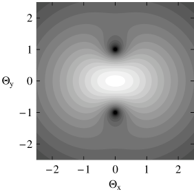
Figure 2: Logarithm of unpolarized radiation intensity (II.3), at $x_{\omega}\to 0$, as a function of $\bm{\Theta}$ (the radiation angle vector in units of $\gamma^{-1}$). The direction of $\bm{q}_{\perp}$ is chosen to be along $y$-axis. A pair of dips (black spots) is manifest. With the increase of $x_{\omega}$ the dips get filled in.

The fully differential radiation probability in all variables $\bm{q}_{\perp}$, $\bm{\Theta}$, $\bm{e}^{\prime}$, $x_{\omega}$ is rarely subject to observation – usually measurements are more inclusive, corresponding to integration over all variables but one or two. Nonetheless, to be able to predict behavior of the integrated probability, it is pre-requisite to understand the features of the integrand. Those main features are listed below.

1. Quasi-Rutherford asymptotics in $\Theta$. At large $\Theta$, radiation intensity (II.3) falls off as $\Theta^{-4}$, i. e. follows essentially the same law as the Rutherford scattering cross-section. This is a general consequence of proportionality of the amplitude to one hard propagator – in the present case of electron, not of a photon. In fact, in Sec. V.2.3 we shall yet encounter a kind of ‘transient asymptotics’ at moderate $\Theta$ (if $x_{\omega}$ is sufficiently small).

2. Polarization alignment along circles at a definite $\hat{\bm{q}}_{\perp}$. It is easy to show by straightforward solution of the ordinary differential equation

   $$\frac{d\Theta_{y}}{d\Theta_{x}}=\frac{G_{ym}\left(\Theta_{x},\Theta_{y}\right)q_{\perp m}}{G_{xm}\left(\Theta_{x},\Theta_{y}\right)q_{\perp m}},$$ (37)

   that curves tangential to the vector field of polarization directions $\mathsf{G}\hat{\bm{q}}_{\perp}$, are a family of circles

   $$\bm{\Theta}^{2}+\mathrm{const}[\bm{q}\times\bm{\Theta}]_{z}=1$$ (38)

   passing through two knot points

   $$\bm{\Theta}_{\pm}=\pm\hat{\bm{q}}_{\perp},\qquad\mathrm{(polarization\,knots,\,intensity\,dips)}$$ (39)

   (see Fig. 3). Along with $\mathsf{G}\hat{\bm{q}}_{\perp}\underset{\bm{\Theta}\to\pm\hat{\bm{q}}_{\perp}}{\approx}\bm{\Theta}\mp\hat{\bm{q}}_{\perp}$, in those points to zero drops the polarization.

3. A pair of intensity dips at a definite $\hat{\bm{q}}_{\perp}$. As is indicated by Eq. (36b), there exists a pair of $\bm{\Theta}$ values, specifically (39), at which $(\mathsf{G}\hat{\bm{q}}_{\perp})^{2}$ turns to zero. Those directions correspond to minima in the radiation intensity at aa definite $\hat{\bm{q}}_{\perp}$ (see Fig. 2).

Features 2, 3, and coincidence of knots and the dips seem to be non accidental. Light on their origin will be thrown in the next subsection.

Figure 3: Photon polarization alignment in the $\bm{\Theta}$ plane. The curves tangential to polarization are mathematical circles. The direction of $\bm{q}_{\perp}$ is along $y$-axis. The polarization degree depends on $x_{\omega}$.

II.4 View from the initial electron rest frame. Stereographic projection

The features of the polarization angular distribution are realized best when we take a view from the initial electron rest frame (IERF).

$$p=(m,\bm{0}).$$ (40)

In the ultra-relativistic limit $e\cdot p\to\infty$. Vector $e$ tends to be light-like:

$$e=\frac{1}{m}(e\cdot p,-e\cdot p,\bm{0}_{\perp}).$$ (41)

The final photon momentum in IERF has all components commensurable

$$k=\left(\Omega,K_{z},\bm{K}_{\perp}\right)\quad\bm{K}_{\perp}=\bm{k}_{\perp},\quad K_{z}=\Omega\cos\Psi,$$ (42)

and $e^{\prime}_{p}$ is a spatial vector orthogonal to $\bm{K}$:

$$e^{\prime}_{p}=(0,\bm{e}^{\prime}_{p}),\quad\bm{e}^{\prime}_{p}\cdot\bm{K}=0,\quad|\bm{e}^{\prime}_{p}|=1.$$ (43)

Vector $q$, which must be orthogonal to $e$, belongs to the light front:

$$q=\left(\frac{p\cdot q}{m},-\frac{p\cdot q}{m},\bm{q}_{\perp}\right),\quad\frac{p\cdot q}{m}\sim x_{\omega}m\quad q^{2}=-\bm{q}^{2}_{\perp},$$ (44)

and in this frame is not transverse, however, vector $e_{p}$, with which the final photon polarization correlates according to Eq. (18a), is transverse:

$$e_{p}=\left(0,0,-\bm{q}_{\perp}\frac{e\cdot p}{p\cdot q}\right)\qquad(e_{p}\cdot q\neq 0).$$ (45)

So, the polarization vector correlator

$$e_{p}\cdot e^{\prime}_{p}\approx-\frac{\bm{q}_{\perp}}{q_{z}}\cdot\bm{e}^{\prime}_{p}$$ (46)

has the usual dipole appearance analogous to that of non-relativistic classical electrodynamics. Therewith, polarization $\bm{e}^{\prime}_{p}$ in IERF is distributed along meridians of a sphere of radiation directions, the polar axis being set by the vector $\bm{q}_{\perp}$.

To reproduce Eqs. (27, 28), it remains to relate $\bm{e}^{\prime}_{p}$ in IERF with $\bm{e}^{\prime}$ in the lab frame. This relation appears to be particularly simple, too. The consided vectors have equal moduli $|\bm{e}^{\prime}_{p}|=|\bm{e}^{\prime}|=1$, and equal components orthogonal to the photon scattering plane $(\bm{K},Oz)$ (because these components are not altered neither by the boost along $Oz$, nor the gauge transformation – translation along 4-vector $q$). Hence, components in the plane $(\bm{K},Oz)$ must have the same norm and be related by a pure rotation. Obviously, since $\bm{e}^{\prime}$ is nearly orthogonal to $Oz$, whereas $\bm{e}^{\prime}_{p}$ is orthogonal to $\bm{K}$, the angle of this rotation is just the angle $\bm{\Psi}$ between $Oz$ and $\bm{K}$:

$$\bm{e}^{\prime}_{p}=\mathsf{R}_{\bm{\Psi}(\bm{\Theta})}\bm{e}^{\prime}$$ (47)

($\mathsf{R}_{\bm{\Psi}(\bm{\Theta})}$ is a product of an operator of gauge transformation and of a boost operator). So, one can view (46) as

$$e_{p}\cdot e^{\prime}_{p}=-\frac{\bm{q}_{\perp}}{q_{z}}\mathsf{G}\bm{e}^{\prime},$$ (48)

where

$$\mathsf{G} = \mathsf{P}_{\perp}\mathsf{R}_{\bm{\Psi}}\mathsf{P}_{\perp}$$

$$= \left(\mathsf{P}_{\perp}-\mathsf{P}_{\bm{k}_{\perp}}\right)+\cos\Psi\mathsf{P}_{\bm{k}_{\perp}}$$

$$\equiv \mathsf{P}_{\perp}-\left(1-\cos\Psi\right)\mathsf{P}_{\bm{k}_{\perp}},$$ (49b)

$\mathsf{P}_{\perp}$ being an operator of projection onto the plane $\perp Oz$, and $\mathsf{P}_{\bm{k}_{\perp}}$ – a projector onto direction $\hat{\bm{k}}_{\perp}$.

Finally, to construct for $\mathsf{G}$ an explicit representation in terms of $\bm{\Theta}$, one first needs to specify $\Psi(\bm{\Theta})$. By definition,

$$\bm{\Theta}=\gamma\frac{\bm{k}_{\perp}}{\omega}.$$ (50)

Here $\omega$, the photon energy in the lab, is related with the energy and momentum by a light-cone dilation

$$\omega=\gamma\left(\Omega+K_{z}\right)\qquad(\mathrm{relativistic\,Doppler\,effect\,eqn.})$$ (51)

Together Eqs. (50, 51) give

$$\bm{\Theta}\left(\frac{\bm{K}}{\Omega}\right)=\frac{\bm{k}_{\perp}}{\Omega+K_{z}}\qquad(\mathrm{ligh\,aberration\,formula}).$$ (52)

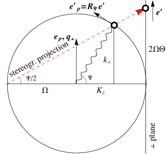
Figure 4: Correspondence between the photon emission angles and polarizations: in the initial electron rest frame ($\bm{\Psi}$, $\bm{e}^{\prime}_{p}$) and in the high-energy transverse plane ($\bm{\Theta}$, $\bm{e}^{\prime}$). For other notations see text. Vectors shown in bold have also components transverse to the plane of the figure. The dashed red line designates the stereographic projection implied by the proportion (52). As a result of projection of the meridional circles from the sphere onto the plane one obtains Fig. 3.

Taking the square of Eq. (52), one relates $\Theta^{2}$ with $\cos\Psi$:

$$\Theta^{2}=\tan^{2}\frac{\Psi}{2}\equiv\frac{1-\cos\Psi}{1+\cos\Psi}.$$ (53)

Inverting this,

$$1-\cos\Psi=\frac{2\Theta^{2}}{1+\Theta^{2}},$$ (54)

and thus the operator entering (49b) is

$$\left(1-\cos\Psi\right)\mathsf{P}_{\bm{k}_{\perp}}=\frac{2}{1+\Theta^{2}}\bm{\Theta}\otimes\bm{\Theta}.$$ (55)

Inserting (55) to (49b), we return to formulas (27, 28).

The benefit from the described alternative view is clarification of geometrical origin of the radiation polarization angular distribution in IERF and in the lab. Relation (52), with the help of Fig. 4, may be interpreted as a projection of unit vectors $\bm{K}/\Omega$, i. e. points on the radiation direction sphere in IERF, onto tangential plane of photon emission angles $\bm{\Theta}$ in the lab, performed from the sphere point opposite to the plane tangency point. Such a construction is known in geometry as stereographic projection Rosenfeld-Sergeeva . It has a few remarkable properties.

Theorem 1.

Points of the sphere symmetric relative to the plane $z=0$ at a stereographic projection pass into points on the plane, symmetric relative to the circle $\left|\bm{\Theta}\right|=1$, in the sense that the product of distances from this points to the origin equals 1.

The proof is trivial: If $\Psi_{1}=\frac{\pi}{2}-\alpha$, $\Psi_{2}=\frac{\pi}{2}+\alpha$, then

$$\Theta_{1}^{2}\Theta_{2}^{2}=\frac{1-\cos\Psi_{1}}{1+\cos\Psi_{1}}\frac{1-\cos\Psi_{2}}{1+\cos\Psi_{2}}=\frac{1-\sin\alpha}{1+\sin\alpha}\frac{1+\sin\alpha}{1-\sin\alpha}=1.$$

The value of Theorem 1 is that it explains unobvious symmetries in the ultrarelativistic particle radiation angular distribution as a manifestation of sufficiently obvious symmetry under Cartesian inversion in the dipole-radiating particle rest frame.

Another useful property is

Theorem 2.

Stereographic projection maps any circle on the sphere to a circle on the plane.

(The proof thereof is more complicated, and we refer for it to the literature Rosenfeld-Sergeeva and we do not reproduce it here). Now, since polarization of dipole radiation in IERF is distributed on the radiation direction sphere along meridional circles, with the polar axis pointing along $\bm{q}_{\perp}$, there is no wonder that bremsstrahlung polarization tangential curves evaluated in Eq. (38) and exhibited in (Fig. 3) are circles, too. (Not surprising either is the existence of the knot pair, which are just projections of the knots on the sphere).

The practical value of the circular polarization alignment pattern will become clear in Sec. V, where we consider polarized radiation angular distributions averaged over momentum transfers $\bm{q}_{\perp}$. The dipole radiation angular distribution shape does not depend on $\left|\bm{q}_{\perp}\right|$, whereas averaging over $\hat{\bm{q}}_{\perp}$ directions implies superimposing polarized radiation intensity distributions rotated with respect to each other. This generally suppresses the radiation polarization, except around angle $\left|\bm{\Theta}\right|=1$, where polarization is rotationally invariant. As for intensity minima of dipole radiation along polar directions in IERF, they make the radiation equatorially concentrated in IERF, which projects into a bar at $\left|\bm{\Theta}\right|<1$ in the lab frame (cf. Fig. 2). That bar will, of course, be rounded by averaging over $\hat{\bm{q}}_{\perp}$. The existence of intensity and polarization maxima can be used for extraction of polarized radiation beams by the angular collimation technique, as will be considered in Sec. V.

III Statistical averaging over momentum transfers in matter

Let us now proceed to description of radiation on a solid target. Momentum $\bm{q}_{\perp}$ imparted to the target is normally beyond detection and has to be integrated over, with the weight $(2\pi)^{-2}\left|A^{\text{diffr}}_{\text{scat}}\left(\bm{q}_{\perp}\right)\right|^{2}=\frac{d\sigma^{\text{diffr}}_{\text{scat}}}{d^{2}q_{\perp}}$, and appropriate averaging over the atomic configurations is due:

$$\left\langle\frac{d\sigma_{\text{rad}}}{d\Gamma_{k}}\right\rangle=\left\langle\int d^{2}q_{\perp}\frac{d\sigma^{\text{diffr}}_{\text{scat}}}{d^{2}q_{\perp}}\frac{dW_{\text{dip}}}{d\Gamma_{k}}\right\rangle.$$ (56)

For a macroscopic target, differential cross-section (56) must be proportional to the target area if the beam is still wider than the target, or to the area of the beam transverse section, if it is narrower than the target (as is a usual practice) and transversely uniform (otherwise, we can consider any beam part uniform relative to target inhomogeneities). Dividing (56) by the interaction area $S$, one obtains a quantity independent of $S$ (but proportional to the target matter density and thickness) and having the meaning of differential probability for the given radiative process to occur per one particle passed through the target.

With $\frac{dW_{\text{dip}}}{d\Gamma_{k}}$ given by Eq. (II.3), in (56) one encounters two basic integrals:

$$\frac{1}{S}\left\langle\int d\sigma^{\text{diffr}}_{\text{scat}}\bm{q}_{\perp}^{2}\right\rangle\! = \!\left\langle\bm{q}_{\perp}^{2}\right\rangle,$$ (57a)

$$\frac{1}{S}\left\langle\!\int\!\!d\sigma^{\text{diffr}}_{\text{scat}}(2q_{\perp m}q_{\perp n}\!-\!\bm{q}_{\perp}^{2}\delta_{mn})\!\!\right\rangle\! = \!\left\langle 2q_{\perp m}q_{\perp n}\!-\!\bm{q}_{\perp}^{2}\delta_{mn}\!\right\rangle,$$

having the meaning of average momentum squares. For our analysis to reach beyond the conventional case of isotropic target, it is prerequisite that average (LABEL:qq-qq) differs from zero. In particular, that allows one to anticipate non-zero polarization of the bremsstrahlung beam as a whole. Physically, this average is related to the azimuthal anisotropy (“ellipticity”) in scattering, even if being not a true measure of the latter due to the radiative character of the averaging (see Subsec. III.2).

III.1 Vector anisotropy parameter and the anisotropy degree

Instead of (LABEL:qq-qq), it is convenient to deal with the ratio of (LABEL:qq-qq) to (57a), which can serve as a direct measure of the scattering asymmetry. This ratio, which is a symmetric traceless tensor in 2 transverse dimensions, can be characterized by the direction of one of its two eigenvectors and the corresponding eigenvalue (another eigenvector will be orthogonal to the first one and correspond to the eigenvalue opposite in sign). Let $\bm{N}$ stand for the eigenvector corresponding to the positive eigenvalue, then we express

$$\frac{\left\langle 2q_{\perp m}q_{\perp n}-\bm{q}_{\perp}^{2}\delta_{mn}\right\rangle}{\left\langle\bm{q}_{\perp}^{2}\right\rangle}\overset{\text{def}}{=}2N_{m}N_{n}\!-\!\bm{N}^{2}\delta_{mn}.$$ (58)

If tensor $\left\langle q_{\perp m}q_{\perp n}\right\rangle$ diagonalizes in axes $x$, $y$, and, say, $\left\langle q^{2}_{y}\right\rangle\geq\left\langle q^{2}_{x}\right\rangle$, then

$$N^{2}=\frac{\left\langle q_{y}^{2}\right\rangle-\left\langle q_{x}^{2}\right\rangle}{\left\langle q_{y}^{2}\right\rangle+\left\langle q_{x}^{2}\right\rangle}$$ (59)

(and $\bm{N}\parallel Oy$). That implies a constraint

$$\bm{N}^{2}\leq 1.$$ (60)

Covariantly, one can infer upper bound (60) by squaring both sides of (58) and taking double trace.

Now, the average differential probability of radiation can be phrased in terms of the introduced vector $\bm{N}$:

$$x_{\omega}\left\langle\frac{dW_{\text{dip}}}{dx_{\omega}d^{2}\Theta}\right\rangle=\frac{\alpha}{4\pi^{2}}\frac{\left\langle\bm{q}^{2}_{\perp}\right\rangle}{m^{2}\left(1+\Theta^{2}\right)^{2}}\qquad\qquad\qquad\qquad\qquad$$

$$\times\bigg{\{}2(1-x_{\omega})\!\left[(G_{im}e^{\prime}_{i})^{2}(1-N^{2})\!+\!2(G_{im}N_{m}e^{\prime}_{i})^{2}\right]\quad\quad$$

$$+x_{\omega}^{2}\bigg{\}}.\qquad$$ (61)

At $N^{2}=1$, Eq. (III.1) essentially coincides with Eq. (II.3). Decomposing also the leftmost unity in braces of Eq. (III.1) as $1\equiv(1-N^{2})+N^{2}$, we get a representation in form of an incoherent mixture of bremsstrahlung on isotropic target with that on an anisotropic one, in proportion $(1-N^{2}):N^{2}$ determiined by the target anisotropy degree. But for polarization characteristics that superposition is non-trivial, inasmuch as the polarization direction and degree does not express as any simple superposition.

III.2 Relaxing the scattering factorization assumption

An important concern at application of bremsstrahlung theory to particle passage through matter is the vulnerability of the scattering factorization condition (6) due to significant target thickness. Fortunately, a way for generalization beyond the factorization is known, which preserves the Dirac matrix structure of the radiation matrix element, only trading the transferred momentum $\bm{q}_{\perp}$ times $A_{\text{scat}}$ for some overlap of initial and final electron wave functions, now involving integration over longitudinal coordinates . To make the text self-contained, we briefly remind the idea behind that generalization Olsen-Maximon-Wergeland .

In the first place, it is suggestive to straightforwardly linearize the primordial factorized matrix element (II.1) with respect to $\bm{q}_{\perp}$:

$$M_{\text{rad}} = \bar{u}^{\prime}\bigg{\{}\!\left(\frac{E}{p^{\prime}\cdot k}-\frac{E^{\prime}}{p\cdot k}\right)e^{\prime*}\cdot\gamma$$ (62)

$$+\frac{e^{\prime*}\cdot\gamma q\cdot\gamma\gamma^{0}}{2p^{\prime}\cdot k}+\frac{\gamma^{0}q\cdot\gamma e^{\prime*}\cdot\gamma}{2p\cdot k}\bigg{\}}u$$

$$\overset{\text{dip}}{\approx} \frac{1}{q_{z}}\bar{u}^{\prime}\bigg{\{}\frac{1}{q_{z}}\left(\bm{v}-\bm{v}^{\prime}\right)\cdot\bm{q}_{\perp}\bm{e}^{\prime*}\cdot\bm{\gamma}$$

$$-\frac{\bm{e}^{\prime*}\cdot\bm{\gamma}\bm{q}_{\perp}\cdot\bm{\gamma}\gamma^{0}}{2E}-\frac{\gamma^{0}\bm{q}_{\perp}\cdot\bm{\gamma}\bm{e}^{\prime*}\cdot\bm{\gamma}}{2E^{\prime}}\bigg{\}}u.\quad$$

Here we have used Eqs. (23) and relations

$$\frac{E}{p^{\prime}\cdot k}-\frac{E^{\prime}}{p\cdot k}=\frac{2EE^{\prime}}{m^{2}\omega}\left[\frac{1}{1+\left(\bm{\Theta}+\frac{\bm{q}}{m}\right)^{2}}-\frac{1}{1+\bm{\Theta}^{2}}\right]\quad$$

$$\approx-\frac{m\omega}{EE^{\prime}q_{z}^{2}}\bm{\Theta}\cdot\bm{q}_{\perp}\approx\frac{1}{q_{z}^{2}}\left(\bm{v}^{\prime}-\bm{v}\right)\cdot\bm{q}_{\perp}.\quad$$ (63)

Whichever the further method of evaluating the spin-averaged probability, the corresponding differential probability is some bilinear form in both $\bm{e}^{\prime}$ and $\bm{q}_{\perp}$, and the answer is already known – it is of the Compton-like form (II.3).

To go beyond the factorization assumption, we have to start with the exact representation of the matrix element in terms of overlap of initial and final electron wave functions in the static field of the target:

$$T=\sqrt{4\pi}ie\int d^{3}re^{-i\bm{k}\cdot\bm{r}}\bar{\psi}^{\prime}(\bm{r})\bm{e}^{\prime*}\cdot\bm{\gamma}\psi(\bm{r}).$$ (64)

In the ultra-relativistic limit, the spin structure of elecron wave functions assumes a field-independent form BLP :

$$\psi(\bm{r})\approx e^{i\bm{p}\cdot\bm{r}}\left(1+\frac{i}{2E}\nabla_{\perp}\cdot\bm{\gamma}\gamma^{0}\right)\varphi(\bm{r})u,$$ (65a)

$$\bar{\psi}^{\prime}(\bm{r})\approx\bar{u}^{\prime}e^{-i\bm{p}^{\prime}\cdot\bm{r}}\left(1-\frac{i}{2E^{\prime}}\gamma^{0}\nabla_{\perp}\cdot\bm{\gamma}\right)\varphi^{\prime*}(\bm{r}),$$ (65b)

where modulating scalar functions $\varphi$, $\varphi^{\prime}$ obey Klein-Gordon type equations

$${\bm{v}}\cdot\nabla\varphi(\bm{r})-V(\bm{r})\varphi(\bm{r})=\frac{1}{2E}\left[\triangle-V^{2}(\bm{r})\right]\varphi(\bm{r}),$$ (66a)

$$-{\bm{v}}^{\prime}\cdot\nabla\varphi^{\prime}(\bm{r})-\!V(\bm{r})\varphi^{\prime}(\bm{r})=\!\frac{1}{2E^{\prime}}\!\left[\triangle-V^{2}(\bm{r})\right]\!\varphi^{\prime}(\bm{r})$$ (66b)

($\bm{v}$ and $\bm{v}^{\prime}$ are the initial and final electron velocities defined by (33), and $V(\bm{r})$ the potential energy of the electron in the electron field of the solid target).

Upon substitution of Eqs. (65) to (64),

$$T_{\text{u.-r.}}=\sqrt{4\pi}ie\int d^{3}re^{i\bm{q}\cdot\bm{r}}\bar{u}^{\prime}\bigg{\{}\bm{e}^{\prime*}\!\cdot\bm{\gamma}\varphi^{\prime*}\varphi\qquad\qquad\qquad$$

$$+\frac{i}{2E}\varphi^{\prime*}\bm{e}^{\prime*}\!\cdot\bm{\gamma}\nabla_{\perp}\!\cdot\bm{\gamma}\gamma^{0}\varphi-\frac{i}{2E^{\prime}}\gamma^{0}\nabla_{\perp}\varphi^{\prime*}\!\cdot\bm{\gamma}\bm{e}^{\prime*}\!\cdot\bm{\gamma}\varphi\bigg{\}}u,$$

first term in the braces of (III.2) appears to be energy-suppressed, because of near orthogonality of $\bm{e}^{\prime*}$ to $\bar{u}^{\prime}\bm{\gamma}u$, and so gives contribution of the same order as the second and third terms of (III.2) (spin corrections) containing energy denominators explicitly. The matrix element non-factorizability implies that in spite of condition $q_{z}\ll q_{\perp}$, one can not neglect $q_{z}$ component in the exponent here, because at the scale $L_{\text{corr}}$ of contributing longitudinal distances we may have $q_{z}L_{\text{corr}}\sim 1$.

It seems that in Eq. (III.2) there are different types of overlaps involving scalar wave functions, but in the dipole approximation they all appear to be interrelated. Indeed,

$$\!\!\int d^{3}re^{i\bm{q}\cdot\bm{r}}\varphi^{\prime*}(\bm{r})\varphi(\bm{r})$$ (68b)

$$\approx \!\!\frac{i}{q_{z}}\int d^{3}re^{i\bm{q}\cdot\bm{r}}({\bm{v}}^{\prime}\cdot\nabla)\left\{\varphi^{\prime*}(\bm{r})\varphi(\bm{r})\right\}$$

$$\equiv \!\!\frac{i}{q_{z}}\int d^{3}re^{i\bm{q}\cdot\bm{r}}\varphi^{\prime*}(\bm{r})\left({\bm{v}}^{\prime}-{\bm{v}}\right)\cdot\nabla\varphi(\bm{r})$$

$$\!\!+\frac{i}{q_{z}}\int d^{3}re^{i\bm{q}\cdot\bm{r}}\left[({\bm{v}}^{\prime}\cdot\nabla\varphi^{\prime*})\varphi+\varphi^{\prime*}{\bm{v}}\cdot\nabla\varphi\right]$$

$$= \!\!\frac{i}{q_{z}}\!\int d^{3}re^{i\bm{q}\cdot\bm{r}}\!\left\{\varphi^{\prime*}\left(\bm{v}^{\prime}-\bm{v}\right)\!\cdot\!\nabla\varphi+\mathcal{O}\left(\frac{q^{2}+V^{2}}{E^{\prime}}\varphi^{\prime*}\varphi\right)\!\right\}$$

$$= \!\!\frac{i}{q_{z}}\left(\bm{v}^{\prime}-\bm{v}\right)\!\cdot\!\!\int d^{3}re^{i\bm{q}\cdot\bm{r}}\varphi^{\prime*}\nabla_{\perp}\varphi\left\{1+\mathcal{O}\!\left(\frac{q_{\perp}}{x_{\omega}m}\right)\!\right\}\!,\quad$$

where in passing to Eq. (LABEL:66a) we have used wave equations (66), and in passing to Eq. (68b) – the estimate $\left|\bm{v}^{\prime}-\bm{v}\right|\sim\frac{x_{\omega}m}{E^{\prime}}$ (cf. Eq. (III.2)). Another type of overlap

$$\int d^{3}re^{i\bm{q}\cdot\bm{r}}\left(\nabla_{\perp}\varphi^{\prime*}(\bm{r})\right)\varphi(\bm{r})$$ (69)

$$= -\int d^{3}re^{i\bm{q}\cdot\bm{r}}\varphi^{\prime*}\nabla_{\perp}\varphi-i\bm{q}_{\perp}\int d^{3}re^{i\bm{q}\cdot\bm{r}}\varphi^{\prime*}\varphi$$

$$\approx \left[-1+\frac{\bm{q}_{\perp}}{q_{z}}\left(\bm{v}^{\prime}-\bm{v}\right)\cdot\right]\int d^{3}re^{i\bm{q}\cdot\bm{r}}\varphi^{\prime*}\nabla_{\perp}\varphi$$

$$= -\int d^{3}re^{i\bm{q}\cdot\bm{r}}\varphi^{\prime*}\nabla_{\perp}\varphi\left\{1+\mathcal{O}\left(\frac{q_{\perp}}{m}\right)\right\}.$$

Thus, the entire overlap (III.2) can be cast in terms of a single overlap between the scalar wave functions

$$\mathfrak{\bm{I}}_{\perp}\left(q_{z},\bm{q}_{\perp}\right)=q_{z}\int d^{3}re^{iq_{z}z+i\bm{q}_{\perp}\cdot\bm{r}_{\perp}}\varphi^{\prime*}(\bm{r})\nabla_{\perp}\varphi(\bm{r}),$$ (70)

specifically:

$$T_{\text{dip}}=\sqrt{4\pi}e\frac{1}{q_{z}}\bar{u}^{\prime}\bigg{\{}\frac{1}{q_{z}}\left(\bm{v}-\bm{v}^{\prime}\right)\cdot\mathfrak{\bm{I}}_{\perp}\bm{e}^{\prime*}\cdot\bm{\gamma}\qquad\qquad$$

$$-\frac{1}{2E}\bm{e}^{\prime*}\cdot\bm{\gamma}\mathfrak{\bm{I}}_{\perp}\cdot\bm{\gamma}\gamma^{0}-\frac{1}{2E^{\prime}}\gamma^{0}\mathfrak{\bm{I}}_{\perp}\cdot\bm{\gamma}\bm{e}^{\prime*}\cdot\bm{\gamma}\bigg{\}}u.$$ (71)

This is observed to have the very same Dirac matrix structure as (62), only with $\mathfrak{\bm{I}}_{\perp}$ emerging in place of $\bm{q}_{\perp}$.

As we see, the recipe for the generalization beyond the scattering factorization is to make in the factorized matrix element

$$T_{\text{fact}}=\sqrt{4\pi}eA^{\text{diffr}}_{\text{scat}}(\bm{q}_{\perp})M_{\text{rad}},$$

with $M_{\text{rad}}$ given by (62), a replacement

$$\bm{q}_{\perp}A^{\text{diffr}}_{\text{scat}}\left(\bm{q}_{\perp}\right)\overset{q_{z}L_{\text{corr}}\sim 1}{\to}\mathfrak{\bm{I}}_{\perp}\left(q_{z},\bm{q}_{\perp}\right),\qquad q_{z}=q_{z}\left(\omega,\bm{\Theta}\right).$$ (72)

Here, factor $e^{iq_{z}z}$ represents the effects of longitudinal coherence sensitivity. Correspondence with the scattering factorization is achieved when this exponential can be put to unity (after a preliminary integration over $z$ by parts, to make the integrand vanish at infinity):

$$\mathfrak{\bm{I}}_{\perp}=i\int d^{2}r_{\perp}e^{i\bm{q}_{\perp}\cdot\bm{r}_{\perp}}\int dze^{iq_{z}z}\frac{\partial}{\partial z}\left[\varphi^{\prime*}(\bm{r})\left(\nabla_{\perp}\right)\varphi(\bm{r})\right]$$

$$\overset{q_{z}L_{\text{corr}}\ll 1}{\to}i\int d^{2}r_{\perp}e^{i\bm{q}_{\perp}\cdot\bm{r}_{\perp}}1(\nabla_{\perp})\varphi(\bm{r}_{\perp},z\gg L_{\text{corr}})\qquad$$

$$=\bm{q}_{\perp}\int d^{2}r_{\perp}e^{i\bm{q}_{\perp}\cdot\bm{r}_{\perp}}\varphi(\bm{r}_{\perp},z\gg L_{\text{corr}}).\qquad\qquad\quad$$ (73)

By the Huygens principle (see, e. g., Huygens ), the latter integral equals to the elastic scattering amplitude, if normalized as in Eq. (10). So,

$$\mathfrak{\bm{I}}_{\perp}\overset{q_{z}L_{\text{corr}}\ll 1}{\to}\bm{q}_{\perp}A^{\text{diffr}}_{\text{scat}}(\bm{q}_{\perp}),$$ (74)

offering a check of the replacement rule consistency (72).

To obtain the spin-averaged probability corresponding to the generalized matrix element (III.2), one needs no special calculation. Obviously, it is a bilinear form in $\mathfrak{\bm{I}}_{\perp}$, which can be retrieved from the factorized bilinear form by replacement $d\sigma^{\text{diffr}}_{\text{scat}}q_{\perp m}q_{\perp n}\to\frac{d^{2}q_{\perp}}{(2\pi)^{2}}\mathfrak{I}_{\perp m}\mathfrak{I}_{\perp n}$. Thereat, the basic averages for our quadratic form promote from (57a, LABEL:qq-qq) to

$$\frac{1}{S}\left\langle\int d\sigma^{\text{diffr}}_{\text{scat}}\bm{q}_{\perp}^{2}\right\rangle\overset{q_{z}L_{\text{corr}}\sim 1}{\to}\frac{1}{S}\left\langle\int\frac{d^{2}q_{\perp}}{(2\pi)^{2}}\left|\mathfrak{\bm{I}}_{\perp}\right|^{2}\right\rangle,$$ (75a)

$$\frac{1}{S}\left\langle\int d\sigma^{\text{diffr}}_{\text{scat}}(2q_{\perp m}q_{\perp n}-\bm{q}_{\perp}^{2}\delta_{mn})\right\rangle\qquad\qquad\quad$$

$$\overset{q_{z}L_{\text{corr}}\sim 1}{\to}\frac{1}{S}\left\langle\int\frac{d^{2}q_{\perp}}{(2\pi)^{2}}\left(2\mathfrak{I}_{\perp m}\mathfrak{I}_{\perp n}-\delta_{mn}\mathfrak{\bm{I}}_{\perp}^{2}\right)\right\rangle.$$ (75b)

The factor $1/S$ in the right-hand sides may be explicitly canceled if $\varphi$ (but not $\varphi^{\prime}$) is substituted by a normalized wave packet in transverse coordinates.

For the modified averages (75a-75) we introduce same shorthands as (57a-LABEL:qq-qq) but with the subscript “rad”:

$$\frac{1}{S}\left\langle\int\frac{d^{2}q_{\perp}}{(2\pi)^{2}}\left|\mathfrak{\bm{I}}_{\perp}\right|^{2}\right\rangle\equiv\left\langle\bm{q}_{\perp}^{2}\right\rangle_{\text{rad}},$$

$$\frac{1}{S}\left\langle\int\frac{d^{2}q_{\perp}}{(2\pi)^{2}}\left(2\mathfrak{I}_{\perp m}\mathfrak{I}_{\perp n}-\delta_{mn}\mathfrak{\bm{I}}_{\perp}^{2}\right)\right\rangle$$

$$\equiv\left\langle 2q_{\perp m}q_{\perp n}-\bm{q}_{\perp}^{2}\delta_{mn}\right\rangle_{\text{rad}}.$$

For expression of the anisotropy parameter, equations (58, 59) remain valid, only with the replacement $\left\langle\bm{q}_{\perp}^{2}\right\rangle\to\left\langle\bm{q}_{\perp}^{2}\right\rangle_{\text{rad}}$:

$$\frac{\left\langle 2q_{\perp m}q_{\perp n}-\bm{q}_{\perp}^{2}\delta_{mn}\right\rangle_{\text{rad}}}{\left\langle\bm{q}_{\perp}^{2}\right\rangle_{\text{rad}}}=2N_{m}N_{n}\!-\!\bm{N}^{2}\delta_{mn},$$ (76)

$$N^{2}=\frac{\left\langle q_{y}^{2}\right\rangle_{\text{rad}}-\left\langle q_{x}^{2}\right\rangle_{\text{rad}}}{\left\langle q_{y}^{2}\right\rangle_{\text{rad}}+\left\langle q_{x}^{2}\right\rangle_{\text{rad}}}.\qquad\qquad$$ (77)

IV The case of azimuthally anisotropic scattering at electron passage through an oriented crystal

Among conceivable applications of the connection between the target intrinsic anisotropy and radiation polarization is the possibility of preparation of a polarized photon beam. For reliability of polarization asymmetry measurements, the beam polarization degree must be high enough, at least a few tens percent, and thence about as high must be $N^{2}$. It is not, however, obvious, whether that sizeable $N^{2}$ can be attained with macroscopic targets. As we had mentioned in the Introduction, the main obstacle thereto is the hard isotropic contribution in scattering. When treating interaction with individual atom as perturbative, in (56) in the integral over $\bm{q}_{\perp}$, or, in an equivalent integral over impact parameters, the contribution from the atomic distance scale $\sim r_{\text{a}}$ is comparable to that from the distances from the nucleus of the order $\sim m^{-1}$, where the impact area is smaller but the acting force, and the generated radiation, is stronger. That familiarly leads to a logarithmic divergence of the integral over $d^{2}q_{\perp}$ from $\frac{d\sigma_{\text{rad}}}{d^{2}q_{\perp}}=\frac{d\sigma_{\text{scat}}}{d^{2}q_{\perp}}dW_{\text{rad}}$, with $dW_{\text{rad}}\propto\bm{q}_{\perp}^{2}$ and $\frac{d\sigma_{\text{scat}}}{d^{2}q_{\perp}}\underset{q_{\perp}\gg r_{\text{a}}^{-1}}{\sim}\bm{q}_{\perp}^{-4}$ (Rutherford tail). Introducing appropriate cutoffs, upper one due to the dipole approximation failure at $q_{\perp}\sim m$, and lower one due to the atomic form-factor regulation, one gets with the logarithmic accuracy

$$\int d^{2}q_{\perp}\bm{q}_{\perp}^{2}\frac{1}{\bm{q}_{\perp}^{4}}=\pi\int_{q_{\perp\text{min}}=r_{\text{a}}^{-1}}^{q_{\perp\text{max}}=m}\frac{dq_{\perp}}{q_{\perp}}=\pi\ln mr_{\text{a}}\approx\pi\ln\frac{1}{\alpha}.$$ (78)

Since in vicinities of the nuclei the scattering is isotropic, the anisotropy parameter $N^{2}$ gets suppressed at least by a factor of $\ln\frac{1}{\alpha}\approx 5$.

A remedy to the encountered suppression could be sought in utilizing oriented crystals. Once one aligns some strong crystallographic axis by a small angle $\chi_{0}\ll 1$ relative to the electron incidence direction (see Fig. 5), the isotropy may persist only up to the distance of transverse separation of atomic nuclei in the string, $\Delta r_{\perp}\sim d_{\text{a}}\chi_{0}$, where $d_{\text{a}}>2r_{\text{a}}$ is the distance between atomic nuclei in the row, while from scale $\Delta r_{\perp}$ up to $r_{\text{a}}$ the scattering should become anisotropic (stronger in the direction transverse to the beam-string plane). At a scale greater than $\chi_{0}d_{\text{a}}$, the cross-section will no longer be a sum of logarithmic cross-sections of scattering on individual atoms, but, rather, the motion will be governed by the aggregate potential of the atoms. The number of atoms overlapping at a given impact parameter is $\sim\frac{r_{\text{a}}}{\chi_{0}d_{\text{a}}}$, and this is the factor the cross-section must increase by, whilst Coulombic logarithms do not develop anymore in this region.

IV.1 Electron interaction with a single atomic string

To verify the above assumption, yet to get an idea of the longitudinal coherence sensitivity, consider first a problem of electron radiation at scattering on a single atomic row under a small angle of incidence. In capacity of initial and final state wave functions in the atomic row potential $V(\bm{r})$, take for simplicity the eikonal approximation (corresponding to the neglect in (66) of the right-hand sides, as well as neglect of the angle between $\bm{v}$ and $\bm{v}^{\prime}$):

$$\varphi(\bm{r})\approx e^{-i\int^{z}_{-\infty}dz^{\prime}V(z^{\prime},\bm{r}_{\perp})},$$ (79a)

$$\varphi^{\prime*}(\bm{r})\approx e^{-i\int^{\infty}_{z}dz^{\prime}V(z^{\prime},\bm{r}_{\perp})},$$ (79b)

$$\varphi^{\prime*}(\bm{r})\varphi(\bm{r})=e^{i\chi_{0}(\bm{r}_{\perp})},\quad\chi_{0}(\bm{r}_{\perp})=-\int^{\infty}_{-\infty}dzV\left(z^{\prime},\bm{r}_{\perp}\right).$$ (80)

Here $\chi_{0}(\bm{r}_{\perp})$ is commonly called the eikonal phase. Substituting (79) into (70), one obtains BKStrakh

$$\mathfrak{\bm{I}}_{\perp}=-iq_{z}\int d^{3}re^{i\bm{q}\cdot\bm{r}+i\chi_{0}(\bm{r}_{\perp})}\nabla_{\perp}\int^{z}_{-\infty}dz^{\prime}V(z^{\prime},\bm{r}_{\perp})\,\,$$

$$=\int d^{2}r_{\perp}e^{i\bm{q}_{\perp}\cdot\bm{r}_{\perp}+i\chi_{0}(\bm{r}_{\perp})}\nabla_{\perp}\int^{\infty}_{-\infty}dze^{iq_{z}z}V(z,\bm{r}_{\perp})\quad$$ (81)

(the second equality results after integration by parts over $z$). The integrals of $|\mathfrak{\bm{I}}_{x}(\bm{q}_{\perp})|^{2}$, $|\mathfrak{\bm{I}}_{y}(\bm{q}_{\perp})|^{2}$ engaged in definition of $N^{2}$ evaluate in a particularly simple form:

$$\int d^{2}q_{\perp}|\mathfrak{\bm{I}}_{x,y}|^{2} = (2\pi)^{2}\int d^{2}r_{\perp}\left|\nabla_{x,y}\int^{\infty}_{-\infty}dze^{iq_{z}z}V\right|^{2}$$ (82)

$$= \int d^{2}q_{\perp}\bm{q}^{2}_{x,y}\left|\int d^{3}re^{i\bm{q}\cdot\bm{r}}V(\bm{r})\right|^{2}.$$

I. e., the eikonal phase actually does not contribute to the given integral, and the result is equivalent to the Born approximation.

Figure 5: Electron small-angle passage through an atomic row. Momentum transfers in $y$ direction (transverse to the picture) are enhanced compared to those in $x$-direction.

To proceed, we have to specify the atomic row potential. Let us, for simplicity, model it by a superposition of individual screened Coulombic potentials. For ia row of $\mathcal{N}$ identical atoms with nucleus charge $Z$, located in the $xz$ plane at an angle $\chi_{0}\ll 1$ to $z$-axis,

$$V_{\text{row}}(\bm{r})=Z\alpha\sum^{\mathcal{N}-1}_{n=0}\frac{e^{-\frac{y^{2}+(x-\chi_{0}d_{\text{a}}n)^{2}+(z-d_{\text{a}}n)^{2}}{r_{\text{a}}}}}{\sqrt{y^{2}+(x-\chi_{0}d_{\text{a}}n)^{2}+(z-d_{\text{a}}n)^{2}}}.$$ (83)

Fourier transform thereof results as

$$\int d^{3}re^{i\bm{q}\cdot\bm{r}}V_{\text{row}}(\bm{r})=\frac{4\pi Z\alpha}{\bm{q}_{\perp}^{2}+r_{\text{a}}^{-2}}\sum^{\mathcal{N}-1}_{n=0}e^{i(q_{z}+\chi_{0}q_{x})d_{\text{a}}n}\qquad$$

$$=\frac{4\pi Z\alpha}{\bm{q}_{\perp}^{2}+r_{\text{a}}^{-2}}e^{i(q_{z}+\chi_{0}q_{x})d_{\text{a}}(\mathcal{N}-1)/2}\frac{\sin\frac{(q_{z}+\chi_{0}q_{x})d_{\text{a}}\mathcal{N}}{2}}{\sin\frac{(q_{z}+\chi_{0}q_{x})d_{\text{a}}}{2}},$$

where in the first denominator term $q_{z}^{2}$ had been neglected compared to $r_{\text{a}}^{-2}$. When squaring (83), the sine ratio factor in a familiar way may be approximated by a sequence of equidistant $\delta$-functions:

$$\frac{\sin^{2}\frac{(q_{z}+\chi_{0}q_{x})d_{\text{a}}\mathcal{N}}{2}}{\sin^{2}\frac{(q_{z}+\chi_{0}q_{x})d_{\text{a}}}{2}}\underset{\mathcal{N}\gg 1}{\approx}\pi\mathcal{N}\sum^{\infty}_{j=-\infty}\delta\left(\frac{(q_{z}+\chi_{0}q_{x})d_{\text{a}}}{2}-\pi j\right)$$

$$=\frac{2\pi\mathcal{N}}{\chi_{0}d_{\text{a}}}\sum^{\infty}_{j=-\infty}\delta\left(q_{x}-\frac{2\pi j}{\chi_{0}d_{\text{a}}}+\frac{q_{z}}{\chi_{0}}\right),\qquad$$

i. e., $q_{x}$-integration reduces to summation over 1-dimensional inverse lattice vectors. As for $q_{y}$-integration, it involves 2 basic integrals:

$$\int^{\infty}_{-\infty}\frac{dq_{y}}{\left(q_{y}^{2}+q_{x}^{2}+r_{\text{a}}^{-2}\right)^{2}}=\frac{\pi}{2\left(q_{x}^{2}+r_{\text{a}}^{-2}\right)^{3/2}}$$ (84a)

for $$\int d^{2}q_{\perp}\left|\mathfrak{\bm{I}}_{x}\right|^{2}$$, and

$$\int^{\infty}_{-\infty}\frac{dq_{y}q_{y}^{2}}{\left(q_{y}^{2}+q_{x}^{2}+r_{\text{a}}^{-2}\right)^{2}}=\frac{\pi}{2\sqrt{q_{x}^{2}+r_{\text{a}}^{-2}}}$$ (84b)

for $\int d^{2}q_{\perp}\left|\mathfrak{\bm{I}}_{y}\right|^{2}$. In the final result, it is convenient to treat in the sum the term $j=0$ separately. It has the meaning of contribution from ‘continuous’ potential, constant along the string. In the higher terms one may neglect $r_{\text{a}}^{-2}$ relative to $\left(\frac{2\pi}{\chi_{0}d_{\text{a}}}\right)^{2}$. Thereby one obtains

$$\frac{1}{\pi\mathcal{N}\left(4\pi Z\alpha\right)^{2}}\!\int\!d^{2}q_{\perp}\left|\mathfrak{\bm{I}}_{y}\right|^{2}=\frac{\pi}{\chi_{0}d_{\text{a}}\sqrt{\frac{q_{z}^{2}}{\chi_{0}^{2}}+r_{\text{a}}^{-2}}}+\sum_{j=1}^{j_{\max}}\frac{1}{j},$$ (85a)

$$\frac{1}{\pi\mathcal{N}\left(4\pi Z\alpha\right)^{2}}\!\int\!d^{2}q_{\perp}\left|\mathfrak{\bm{I}}_{x}\right|^{2}=\frac{\pi q_{z}^{2}}{\chi_{0}^{3}d_{\text{a}}\left(\frac{q_{z}^{2}}{\chi_{0}^{2}}+r_{\text{a}}^{-2}\right)^{\!3/2}}+\sum_{j=1}^{j_{\max}}\frac{1}{j}.$$ (85b)

The summation upper limit $j_{\max}$ is determined by the same principle as that of integration in (78) – it is set at $q_{x}\sim m$, so

$$j_{\max}=j_{\max}(\chi_{0})\sim\frac{\chi_{0}d_{\text{a}}}{2\pi}m\sim 20\,\chi_{0},$$

$$\sum_{j=1}^{j_{\max}(\chi_{0})}\frac{1}{j}\approx\max\left\{1,\ln\left[e^{C_{E}}j_{\max}(\chi_{0})\right]\right\}\overset{\text{def}}{=}L_{0}\,(\chi_{0}).$$

For scattering on a single string at zero temperature, no additional averaging over string ensembles is required, and substitution of (85a, 85b) to (77) gives the result for the azimuthal anisotropy parameter

$$N^{2}=\frac{1}{1+2\frac{q_{z}^{2}r_{\text{a}}^{2}}{\chi_{0}^{2}}+\frac{2}{\pi}\left(1+\frac{q_{z}^{2}r_{\text{a}}^{2}}{\chi_{0}^{2}}\right)^{3/2}\frac{\chi_{0}d_{\text{a}}}{r_{\text{a}}}L_{0}(\chi_{0})}$$ (86)

(we remind that $q_{z}\left(\omega,\bm{\Theta}\right)$ is defined by Eq. (24)).

Based on the above explicit formula, let us now assess the effects of scattering on individual nuclei and of the longitudinal coherence sensitivity. In the denominator of (86), terms $\frac{q_{z}^{2}r_{\text{a}}^{2}}{\chi_{0}^{2}}$ reflect the effect of coherence sensitivity on the anisotropy of radiation distribution. Apparently, increase of $q_{z}$ through $\omega$ always suppresses the anisotropy. The last term, containing $L_{0}$, accounts for effects of the string discreteness, which are also suppressing the anisotropy. But due to the factor $\frac{\chi_{0}d_{\text{a}}}{r_{\text{a}}}$ (inverse coherence enhancement factor), this effect weakens as $\chi_{0}$ decreases, and even at angles as large as

$$\chi_{0}\sim 0.2\,\text{rad}\sim 10^{\circ},\qquad L_{0}(\chi_{0})\simeq 2$$ (87)

one has $N^{2}\sim 0.5$, provided $\frac{q_{z}r_{\text{a}}}{\chi_{0}}<\frac{1}{2}$. In fact, at impact angles (87), and $q_{z}\sim x_{\omega}m/\gamma$, the ratio $\frac{q_{z}r_{\text{a}}}{\chi_{0}}\sim\frac{x_{\omega}}{2\alpha\gamma\chi_{0}}$ quantifying the longitudinal coherence effect on the anisotropy, will be small if

$$\gamma\geq\frac{x_{\omega}}{\alpha\chi_{0}}10^{3}x_{\omega}\quad\Rightarrow\quad N\approx N(q_{z}\to 0)=\mathrm{const}.$$ (88)

In this case, $N^{2}$ can be regarded as independent of $q_{z}$, and therethrough of the emitted photon momentum.

From the estimate (87) one can further infer the sufficient crystal quality, the crystal orientation precision and the beam collimation degree; we will not discuss these items in detail herein.

IV.2 Multiple scattering on atomic strings

To be realistic, at electron passage through a real oriented crystal, interaction with one string is not the whole story but only an elementary act. Multiple interactions can affect the distribution function in scattering angles, and yet, in case of periodical string hitting, modify the radiation spectrum through the periodic structure form-factor.

For successive scattering on atomic rows with nearly continuous string potentials, the modulus of the angle between the row and the electron motion direction is actually approximately conserved (transverse energy conservation). Hence, in multiple scattering on mutually parallel strings the electron momentum will diffuse over a cone with the axis along the string direction (‘doughnut’ scattering doughnut ), and for a sufficiently thick target the scattering must isotropize. To keep the scattering azimuthal anisotropy significant, one should not permit the electron passage to such late a stage. The allowable target thickness $L$ is estimated by assuming that at this distance the electron interacts with $L\frac{\chi_{0}}{d_{\text{a}}}$ strings, scattering on each one through a small angle

$$\chi_{1}\sim\frac{F_{0}}{E}\frac{r_{\text{a}}}{\chi_{0}}=\frac{2V_{0}}{E\chi_{0}},$$

whence the change of the azimuth $\frac{\chi_{1}}{\chi_{0}}$ needs be $\ll 1$, too. Then, the mean square of the scattering azimuthal angle on a sequence of (statistically independent) strings, $L\frac{\chi_{0}}{d_{\text{a}}}\frac{\chi_{1}^{2}}{\chi_{0}^{2}}$, is required to be less than unity. So, the condition for the target thickness ensues as

$$L<L_{\text{isotr}}\!\sim d_{\text{a}}\frac{\chi_{0}}{\chi_{1}^{2}}\sim d_{\text{a}}\frac{E^{2}\chi_{0}^{3}}{4V_{0}^{2}}\sim\frac{d_{\text{a}}}{4\alpha^{4}}\chi_{0}^{3}\gamma^{2}\quad\left(\frac{m}{V_{0}}\!\sim\!\frac{1}{\alpha^{2}}\right),$$ (89)

where $\frac{d_{\text{a}}}{4\alpha^{4}}\sim\mathrm{1-2\,cm}$. At $\gamma$ satisfying (88), with $\chi_{0}$ of the order of (87), the effect of doughnut isotropization is weak.

On the other hand, if strings are encountered along the particle path periodically (‘string of strings’ radiation doughnut , similar to coherent bremsstrahlung Diambrini ), then even at $\frac{q_{z}r_{\text{a}}}{\chi_{0}}<\frac{1}{2}$ one can still have $\frac{q_{z}d_{\text{s}}}{\chi_{0}}\sim 1$, with $d_{\text{s}}$ the distance between the strings. Then, coherence effects in radiation may develop on a larger spatial scale. If the period of string sequence is equal to the photon formation length (5) at some $\omega$, $\theta$, then the spectrum contains a resonance radiation peak at this frequency. Within the peak, the value of $q_{z}$, and therewith of $\bm{q}_{\perp}$, may be regarded as certain (the ‘point effect’ in coherent bremsstrahlung Diambrini ). Then, the azimuthal asymmetry degree, again, would approach unity, minus corrections on thermal atom oscillations, lattice defects, etc.

To conclude this section, let us remark that physically interesting examples of media with non-zero $N^{2}$, of course, are not restricted to string-like configurations described above. There are many other configurations (textured polycrystals, bent crystals BondCBBC , polarized non-spherical nuclei, etc.), which even if aren’t particularly convenient for polarized photon beam production, but are physically interesting by themselves. Such systems allow diagnostics by the (polarized) bremsstrahlung. The bremsstrahlung properties for such systems must be qualitatively similar, since they are characterized by the aggregate vector $\bm{N}$ only. Analysis of these properties depending on the parameter $N$, as it assumes intermediate values $0<N<1$, is carried out in the next section.

V Bremsstrahlung polarization observables

In general, function $\bm{N}\left(\omega,\Theta\right)$ is model-dependent, and models, in principle, may vary. To derive model-independent conclusions, let us for the rest of this paper assume $\bm{N}$ to be a constant (see condition (88)), though arbitrary parameter. Therewith, we will investigate influence of $\bm{N}$ on the radiation intensity and on polarization, both in the integral photon beam and in the detail of angular distribution.

Upon replacement in (III.1) $\left\langle\bm{q}^{2}_{\perp}\right\rangle\to\left\langle\bm{q}^{2}_{\perp}\right\rangle_{\text{rad}}$, the radiation intensity differential distribution reads

$$x_{\omega}\left\langle\frac{dW_{\text{dip}}}{dx_{\omega}d^{2}\Theta}\right\rangle=\frac{\alpha}{4\pi^{2}}\frac{\left\langle\bm{q}^{2}_{\perp}\right\rangle_{\text{rad}}}{m^{2}\left(1+\Theta^{2}\right)^{2}}\qquad\qquad\qquad\quad$$

$$\times\!\left\{{2(1\!-\!x_{\omega})}\!\left[(G_{im}e^{\prime}_{i})^{2}(1\!-\!N^{2})\!+\!2(G_{im}N_{m}e^{\prime}_{i})^{2}\right]\!+\!x_{\omega}^{2}\right\}\!.$$

To separate the unpolarized part and the polarization, one needs to split the dependence of Eq. (III.1) on $\bm{e}^{\prime}$ into the isotropic and the quadrupole parts, writing

$$(G_{im}e^{\prime}_{i})^{2} = 1-\frac{4(\bm{\Theta}\cdot\bm{e}^{\prime})^{2}}{\left(1+\Theta^{2}\right)^{2}}$$

$$\equiv \frac{1+\Theta^{4}+2\left(\Theta^{2}\delta_{ij}-2\Theta_{i}\Theta_{j}\right)e^{\prime}_{i}e^{\prime}_{j}}{(1+\Theta^{2})^{2}},$$

and

$$2(G_{im}N_{m}e^{\prime}_{i})^{2}\qquad\quad\qquad\quad\qquad\quad\qquad\quad\qquad\quad\qquad\quad$$

$$\equiv(G_{lm}N_{m})^{2}+\left[2G_{im}N_{m}G_{jn}N_{n}-(G_{lm}N_{m})^{2}\delta_{ij}\right]e^{\prime}_{i}e^{\prime}_{j},$$

where

$$(G_{lm}N_{m})^{2}=N^{2}-\frac{4(\bm{N}\cdot\bm{\Theta})^{2}}{\left(1+\Theta^{2}\right)^{2}}.$$

As a result, we bring Eq. (V) to the form

$$x_{\omega}\left\langle\frac{dW_{\text{dip}}}{dx_{\omega}d^{2}\Theta}\right\rangle=\frac{1}{2}x_{\omega}\left\langle\frac{dW_{\text{unpol}}}{dx_{\omega}d^{2}\Theta}\right\rangle\qquad\qquad\qquad\qquad$$

$$+\frac{\alpha}{4\pi^{2}}\frac{\left\langle\bm{q}^{2}_{\perp}\right\rangle_{\text{rad}}}{m^{2}\left(1+\Theta^{2}\right)^{2}}\frac{2(1-x_{\omega})}{x_{\omega}^{2}}\left(2T_{ij}-T\delta_{ij}\right)e^{\prime}_{i}e^{\prime}_{j},\quad$$ (91)

with tensor $T_{ij}$ emerging as

$$T_{ij}=-\frac{2(1-N^{2})}{\left(1+\Theta^{2}\right)^{2}}\Theta_{i}\Theta_{j}+G_{im}N_{m}G_{jn}N_{n},$$ (92)

$T$ its trace

$$T=T_{ii}=-\frac{2(1-N^{2})\Theta^{2}}{\left(1+\Theta^{2}\right)^{2}}+(G_{lm}N_{m})^{2},$$ (93)

and the unpolarized part of Eq. (V) (equal to Eq. (V) summed up over the independent polarization states $e^{\prime}_{n}$)

$$x_{\omega}\left\langle\frac{dW_{\text{unpol}}}{dx_{\omega}d^{2}\Theta}\right\rangle=x_{\omega}\sum_{\bm{e}^{\prime}}\left\langle\frac{dW_{\text{dip}}}{dx_{\omega}d^{2}\Theta}\right\rangle\quad\qquad\qquad\qquad$$

$$=\frac{\alpha}{2\pi^{2}}\frac{\left\langle\bm{q}^{2}_{\perp}\right\rangle_{\text{rad}}}{m^{2}\left(1+\Theta^{2}\right)^{2}}\qquad\qquad\qquad\qquad\qquad\qquad\qquad$$

$$\times\!\left\{2(1-x_{\omega})\frac{1+\Theta^{4}+2\left[N^{2}\Theta^{2}-2(\bm{N}\cdot\bm{\Theta})^{2}\right]}{\left(1+\Theta^{2}\right)^{2}}+x_{\omega}^{2}\!\right\}\!.$$

V.1 Spectrum and net polarization of the integral radiation cone

If angular resolution of the emitted radiation is not pursued in the experiment (which may become impractical at $\gamma>10^{4}$), and only the natural collimation due to emission from an ultra-relativistic particle is utilized, one must integrate Eq. (V) over the small radiation angles, i. e., a $\bm{\Theta}$ plane. The angular integrations are carried out with the aid of the basic integrals

$$\int\frac{d\phi_{\bm{\Theta}}}{2\pi}\Theta_{i}\Theta_{j}=\frac{1}{2}\delta_{ij}\Theta^{2},$$

$$\int\frac{d\phi_{\bm{\Theta}}}{2\pi}\Theta_{i}\Theta_{j}\Theta_{l}\Theta_{m}=\frac{1}{8}\left(\delta_{ij}\delta_{lm}+\delta_{il}\delta_{jm}+\delta_{im}\delta_{jl}\right)\Theta^{4},$$ (95)

$$\int_{0}^{\infty}\frac{d\Theta^{2}(\Theta^{2})^{m}}{\left(1+\Theta^{2}\right)^{2+n}}=\frac{m!(n-m)!}{(n+1)!}.$$ (96)

The result is

$$x_{\omega}\left\langle\frac{dW_{\text{dip}}}{dx_{\omega}}\right\rangle=\frac{1}{2}\int d\Theta^{2}\frac{d\phi_{\bm{\Theta}}}{2\pi}x_{\omega}\left\langle\frac{dW_{\text{dip}}}{dx_{\omega}d^{2}\Theta}\right\rangle\qquad\quad\quad$$

$$=\frac{\alpha\left\langle\bm{q}_{\perp}^{2}\right\rangle_{\text{rad}}}{4\pi m^{2}}\!\left\{\frac{2}{3}(1-x_{\omega})\!\left[2+2(\bm{N}\cdot\bm{e}^{\prime})^{2}\!-\!N^{2}\right]+x_{\omega}^{2}\right\}\!.$$

The unpolarized, Bethe-Heitler’s spectral intensity (which otherwise might be obtained by integrating Eq. (V)) ensues

$$J_{\mathrm{BH}}\left(x_{\omega}\right) = x_{\omega}\left\langle\frac{dW_{\text{unpol}}}{dx_{\omega}}\right\rangle=x_{\omega}\sum_{\bm{e}^{\prime}}\left\langle\frac{dW_{\text{dip}}}{dx_{\omega}}\right\rangle$$ (98a)

$$= \frac{\alpha\left\langle\bm{q}_{\perp}^{2}\right\rangle_{\text{rad}}}{2\pi m^{2}}\left\{\frac{4}{3}\left(1-x_{\omega}\right)+x_{\omega}^{2}\right\}\qquad\quad$$

$$\equiv \frac{\alpha\left\langle\bm{q}_{\perp}^{2}\right\rangle_{\text{rad}}}{2\pi m^{2}}\frac{E^{\prime}}{E}\left(\frac{E^{\prime}}{E}+\frac{E}{E^{\prime}}-\frac{2}{3}\right)\!$$ (98b)

(see Fig. 6, upper dashed curve). Therein the dependence on $\bm{N}$ completely drops out – quite naturally, recalling that $\bm{N}$ is representative of the quadrupole dependence on $\bm{q}_{\perp}$, while after integration over $\bm{\Theta}$ it can only be contracted with the quadrupole tensor dependence on $\bm{e}^{\prime}$ (as Eq. (V.1) indicates), but after summation over $\bm{e}^{\prime}$ all that averages to zero. The integral of the $x_{\omega}$-dependent expression in Eq. (98a) is unity:

$$\int_{0}^{1}dx_{\omega}\left\{\frac{4}{3}\left(1-x_{\omega}\right)+x_{\omega}^{2}\right\}=1.$$

Figure 6: Dashed curve – Bethe-Heitler spectral distribution of bremsstrahlung energy (Eq. (98a)), normalized to its value at $x_{\omega}=0$. Oblique dashed line – the polarized fraction of the radiation spectrum divided by $N^{2}$, for the case of constant $\bm{N}$. Solid curve – net polarization of the photon beam (Eq. (99b)) divided by $N^{2}$. (Polarization orientation is $\parallel\bm{N}$).

Finally, the polarization deduced from Eq. (V.1) is directed parallel to $\bm{N}$

$$\bm{t}_{+}\parallel\bm{N},$$ (99a)

and its degree equals

$$\mathtt{P}_{\text{net}}=\frac{N^{2}}{2}\frac{1}{1+\frac{3x_{\omega}^{2}}{4(1-x_{\omega})}}.$$ (99b)

The semi-classical limit ($x_{\omega}\to 0$) of (99b) at $N=1$ agrees with the polarization $\frac{1}{2}$ of dipole radiation from a classical charged particle in a planar undulator BKStrakh . The $x_{\omega}$-dependent factor describes the polarization suppression due to the photon recoil. The function $\mathtt{P}_{\text{net}}/N^{2}$ is shown in Fig. 6 by solid curve.

The practical value of the non-zero net polarization is that once there is a target with sizeable $N^{2}/2$, it suffices for obtaining a polarized gamma-ray beam without the need for narrow collimation and particular target thinness Uberall . The common known drawback of incoherent bremsstrahlung radiation is its continuous spectrum, but that may be overcome by measurement of the energies of all final products of the induced reactions.

Vice versa, measurement of the net polarization may be used as a technique for empirical determination of $\bm{N}$ for a given target. If one’s aim is to obtain a polarized photon beam, this will be equivalent to the source calibration in situ.

V.2 Angular distributions

V.2.1 Unpolarized intensity

Inspection of Eq. (V) reveals that the azimuthal anisotropy embodied by the quadrupole dependence on the angle $\phi_{\bm{\Theta}}$ between $\bm{\Theta}$ and $\bm{N}$,

$$N^{2}\Theta^{2}-2(\bm{N}\cdot\bm{\Theta})^{2}=-N^{2}\Theta^{2}\cos 2\phi_{\bm{\Theta}},$$

is sizeable only when $N^{2}\sim 1$, and only at angles $\Theta\sim 1$. At $\Theta\ll 1$, or $\Theta\gg 1$, the unpolarized radiation differential intensity isotropizes and becomes independent of $N^{2}$ at all (however, the polarization will not be neither isotropic, nor small there – see Eq. (108) below). The distribution of unpolarized intensity (V) in the $\bm{\Theta}$ plane, for constant $\bm{N}$, at examplary values $N^{2}=\frac{1}{2}$ and $x_{\omega}=\frac{1}{3}$, is illustrated in Fig. 7. As compared with Fig. 2, no dips are left at $N^{2}$ that small (and $x_{\omega}$ that large), but there still remains a noticeable azimuthal anisotropy, the radiation intensity being enhanced in a bar orthogonal to $\bm{N}$, because dipole radiation intensity is known to be largest in directions orthogonal to that of the acceleration (the much greater deflection due to the transverse recoil from the photon emission proves to be of no consequence there). In contrast, electron multiple scattering diffusion in the sample will be fastest in direction parallel to $\bm{N}$.

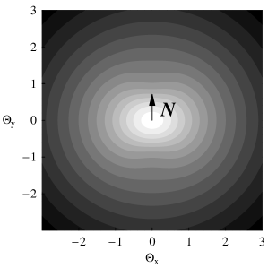
Figure 7: Logarithm of the unpolarized differential cross-section, as a function of $\bm{\Theta}$ (radiation angles in units $\gamma^{-1}$), at $\bm{N}$ independent of $\bm{\Theta}$, for $N^{2}=\frac{1}{2}$, $x_{\omega}=\frac{1}{3}$.

If resolution of radiation angles is feasible in the experiment, measurement of the radiation azimuthal anisotropy (say, at $\Theta\approx 1$) may offer a method for parameter $\bm{N}$ determination for a given target. Other methods are based on polarization measurements, needing no electron detection. We now proceed with discussion of the polarization angular distribution.

V.2.2 Polarization

As long as linear polarization is a vector quantity, to handle it practically, it is best to know its absolute magnitude (degree) and the direction. However, those variables are not in a linear relation to the calculated differential probability, which, after momentum averaging in matter, turns to a generic kind of tensor in $\bm{e}^{\prime}$ – see (V). This may prompt one to deal with polarization asymmetries in some fixed coordinate frame, such as Stokes parameters. But actually, in 2 transverse dimensions expressing the polarization direction explicitly is not difficult at all, involving at the most quadratic equations.

From Eq. (V), the polarization degree is extracted as an asymmetry

$$\mathtt{P}(\bm{\Theta},x_{\omega};\bm{N}) \overset{\text{def}}{=} \frac{\underset{\bm{e}^{\prime}}{\max}\left\langle\frac{dW_{\text{dip}}}{d\Gamma_{k}}\right\rangle-\underset{\bm{e}^{\prime}}{\min}\left\langle\frac{dW_{\text{dip}}}{d\Gamma_{k}}\right\rangle}{\underset{\bm{e}^{\prime}}{\max}\left\langle\frac{dW_{\text{dip}}}{d\Gamma_{k}}\right\rangle+\underset{\bm{e}^{\prime}}{\min}\left\langle\frac{dW_{\text{dip}}}{d\Gamma_{k}}\right\rangle}$$ (100)

$$= \frac{\alpha}{2\pi^{2}}\frac{\left\langle\bm{q}^{2}_{\perp}\right\rangle_{\text{rad}}(1-x_{\omega})}{m^{2}\left(1+\Theta^{2}\right)^{2}}\frac{2\lambda_{+}[T_{ij}]}{x_{\omega}\left\langle\frac{dW_{\text{unpol}}}{dx_{\omega}d^{2}\Theta}\right\rangle}\quad$$

$$= \frac{\lambda_{+}[T_{ij}]}{\frac{x_{\omega}^{2}}{2(1-x_{\omega})}+\frac{1+\Theta^{4}+2\left[N^{2}\Theta^{2}-2(\bm{N}\cdot\bm{\Theta})^{2}\right]}{\left(1+\Theta^{2}\right)^{2}}},$$

where $\lambda_{+}[T_{ij}]$ is the positive eigenvalue of tensor $\left(2T_{ij}-T\delta_{ij}\right)$. In terms of the latter, $\lambda_{+}$ may be expressed as

$$\lambda_{+}=\sqrt{\frac{1}{2}\left(2T_{ij}-T\delta_{ij}\right)\left(2T_{ij}-T\delta_{ij}\right)}\equiv\sqrt{2T_{ij}T_{ij}-T^{2}}.$$ (101)

In our case (92), tensor $T_{ij}$ is formed by two vectors:

$$T_{ij}=a_{i}a_{j}-b_{i}b_{j}$$ (102)

with

$$a_{i}=G_{im}N_{m},\qquad b_{i}=\frac{\sqrt{2(1-N^{2})}}{1+\Theta^{2}}\Theta_{i}$$ (103)

(those vectors are not mutually orthogonal, in general). Substituting Eq. (102) to Eq. (101), one straightforwardly evaluates

$$\lambda_{+} = \sqrt{(\bm{a}^{2}-\bm{b}^{2})^{2}+4[\bm{a}\times\bm{b}]^{2}}$$ (104a)

$$\equiv \left|\bm{a}-\bm{b}\right|\left|\bm{a}+\bm{b}\right|\qquad$$ (104b)

Eigenvectors of a tensor of the form (102) can be expressed covariantly in terms of the vectors $\bm{a}$, $\bm{b}$:

$$\bm{t}_{\pm} \parallel 2(\bm{a}\cdot\bm{b})\bm{a}-(\bm{a}^{2}+\bm{b}^{2})\bm{b}\pm\lambda_{+}\bm{b}$$ (105a)

$$\parallel 2(\bm{a}\cdot\bm{b})\bm{b}-(\bm{a}^{2}+\bm{b}^{2})\bm{a}\mp\lambda_{+}\bm{a},$$ (105b)

$$\bm{t}_{+}\perp\bm{t}_{-}$$ (105c)

(the coefficients at $\bm{a}$, $\bm{b}$ in (105a-105b) are found by solving a system of two linear equations).

Substitution of (103) into Eqs. (104a, 105a) leads to representations

$$\lambda_{+} = \sqrt{\left[N^{2}-\frac{4(\bm{N}\cdot\bm{\Theta})^{2}+2(1-N^{2})\Theta^{2}}{\left(1+\Theta^{2}\right)^{2}}\right]^{2}+\frac{8(1-N^{2})[\bm{\Theta}\times\bm{N}]^{2}}{\left(1+\Theta^{2}\right)^{2}}},$$ (106)

$$\bm{t}_{\pm} \parallel 2\frac{1-\Theta^{2}}{1+\Theta^{2}}(\bm{N}\cdot\bm{\Theta})\bm{N}+\left[\frac{2\left[2(\bm{N}\cdot\bm{\Theta})^{2}+N^{2}-1\right]\Theta^{2}}{\left(1+\Theta^{2}\right)^{2}}-N^{2}\pm\lambda_{+}\right]\bm{\Theta}.$$ (107)

One may note that at $\Theta\gg 1/N$ the polarization picture simplifies, tending to

$$\mathtt{P}\to N^{2}\mathtt{P}_{\text{max}}(x_{\omega}),\quad\bm{t}_{+}\parallel\bm{N}-\frac{2(\bm{N}\cdot\bm{\Theta})}{\Theta^{2}}\bm{\Theta}.\quad(\Theta\gg 1/N)$$ (108)

So, the polarization distribution shape in this region is the same as in extremely anisotropic case $|\bm{N}|=1$, or for non-averaged $x_{\omega}\frac{dW_{\text{rad}}}{dx_{\omega}d^{2}\Theta}$ at definite $\bm{q}_{\perp}$ (see Sec. II, Fig. 3), except that the polarization degree is $\propto N^{2}$ . However at practice, since $N$ decreases with increasing $\Theta$ (according to Eq. (86), $N\underset{\Theta\to\infty}{\sim}\Theta^{-2}$), at sufficiently large $\Theta$ isotropy must set in. We refrain from studying the transition to this regime insofar as it is model- and process- dependent.

The complete polarization picture (the polarization degree and direction), is shown in Fig. 8. It appears to have a richer structure than the corresponding unpolarized intensity in Fig. 7. A novel feature at $N<1$ is that the knot points (39) split, admitting the “polarization flow” into the gaps. Polarization zero positions now can be found from setting $\mathtt{P}$, or $\lambda_{+}$ as given by Eq. (106), equal to zero. That yields

$$\bm{\Theta}_{>} = \pm\frac{\bm{N}}{N^{2}}\sqrt{1+\sqrt{1-N^{4}}},$$ (109)

$$\bm{\Theta}_{<} = \pm\frac{\bm{N}}{N^{2}}\sqrt{1-\sqrt{1-N^{4}}}.$$ (110)

The mean geometric value of distances to these points from the origin equals 1:

$$\sqrt{\Theta_{>}\Theta_{<}}=1\$$ (111)

(this can be traced to the fact that on the sphere of radiation directions in the initial electron rest frame those points are located symmetrically relative to plane $z=0$, and upon the stereographic projection they become conjugate with respect to the unit circle, see Sec. II.4, Theorem 1), whereas the gap width

$$\Theta_{>}-\Theta_{<}=\frac{\sqrt{2}\sqrt{1-N^{2}}}{N}$$ (112)

exhibits “threshold behavior” as $N$ departs from 1. However, now the points of zero polarization do not correspond to any dips in the radiation intensity (cf. Fig. 7).

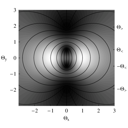
Figure 8: Angular distribution of the polarization degree (density plot) and orientation (black curves) at $\bm{N}$ independent of $\bm{\Theta}$, for $N^{2}=\frac{1}{2}$, $x_{\omega}=\frac{1}{3}$. For principal profiles of this distribution – see Figs. 9(a), 9(b) below, middle curves. The direction of $\bm{N}$ is vertical. At $|\bm{\Theta}|\to\infty$ polarization degree tends to a constant value $N^{2}$. The unpolarized radiation intensity for the same parameters is displayed in Fig. 7.

Determination of the bremsstrahlung polarization zeroes may serve as another calibration method for the parameter $\bm{N}$. The virtue of this method is that it does not require absolute measurements of intensity, but of the angles only. When $N$ is small, it is convenient to measure it through measurement of $\Theta_{<}$, which is $\Theta_{<}\sim N$, in contrast to $\mathtt{P}_{\text{net}}\sim N^{2}$. Vice versa, when $N^{2}$ is close to 1 (say, in coherent bremsstrahlung), it is convenient to measure (112) (due to the square root dependence).

The analytic form of the polarization tangential curves in general case is complicated (though, stereographic projection can offer some simplifications), and we do not contemplate determining it here. At least, at $\Theta=1$ it is apparent that $\bm{t}_{-}\parallel\bm{\Theta}$, hence $\bm{t}_{+}\perp\bm{\Theta}$, i. e. , polarization direction is steered along the unit circle, anyway.

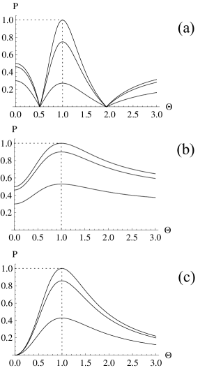
Figure 9: (a). Polarization degree at $\bm{\Theta}\parallel\bm{N}$ for $\bm{N}$ independent of $\omega$, $\bm{\Theta}$, having magnitude $N^{2}=\frac{1}{2}$, and for photon energy fractions $x_{\omega}=0,\frac{1}{3}$, and $\frac{2}{3}$ (top to bottom). Orientation of the polarization depends on the interval – see Eqs. (114). (b). Same as (a), except that profile $\bm{\Theta}\perp\bm{N}$ is shown. Polarization orientation is $\parallel\bm{N}$. (c). Polarization of bremsstrahlung on an isotropic target ($N=0$) for same values of $x_{\omega}$.

To gain more quantitative understanding of the profile of polarization distribution, it is instructive to examine its two principal profiles: $\bm{\Theta}\parallel\bm{N}$ and $\bm{\Theta}\perp\bm{N}$. In those cases, $\bm{a}\parallel\bm{b}$, or $\bm{a}\perp\bm{b}$, owing to which Eqs. (106, 107) substantially simplify.

(i) If $\bm{\Theta}\parallel\bm{N}$,

$$\lambda_{+}=\left|N^{2}-\frac{2\Theta^{2}(1+N^{2})}{(1+\Theta^{2})^{2}}\right|,$$ (113)

$$\bm{t}_{+}\parallel\bm{N} \text{if either}\quad|\bm{\Theta}|<\Theta_{<},\,\,\,\text{or}\,\,\,|\bm{\Theta}|>\Theta_{>},\qquad$$ (114a)

$$\bm{t}_{+}\perp\bm{N} \text{in the interval}\quad\Theta_{<}<|\bm{\Theta}|<\Theta_{>}$$ (114b)

(Eq. (114a) is inferred from Eq. (107) with the upper sign, Eq. (114b) – from Eq. (107) with the lower sign). The polarization degree (100) through (113) reduces to

$$\mathtt{P}=\frac{\left|N^{2}\left(1+\Theta^{4}\right)-2\Theta^{2}\right|}{1+\Theta^{4}-2N^{2}\Theta^{2}+\frac{x_{\omega}^{2}}{2(1-x_{\omega})}\left(1+\Theta^{2}\right)^{2}}.$$ (115)

This function is displayed in Fig. 9(a). It drops to zero at $\Theta=\Theta_{+<},\Theta_{+>}$, has maxima at $\Theta=0$ and $\Theta=\infty$, where it achieves the same values

$$\mathtt{P}(\bm{\Theta}=0)=\mathtt{P}(\bm{\Theta}=\infty)=N^{2}\mathtt{P}_{\text{max}}(x_{\omega})=\frac{2N^{2}\left(1-x_{\omega}\right)}{1+\left(1-x_{\omega}\right)^{2}},$$ (116)

and at $\Theta^{2}=1$, where

$$\mathtt{P}(\bm{\Theta}=\pm\bm{N}/|\bm{N}|)=\frac{1}{1+\frac{x_{\omega}^{2}}{(1-x_{\omega})(1-N^{2})}}.$$ (117)

(ii) In the case of orthogonal profile $\bm{\Theta}\perp\bm{N}$,

$$\bm{t}_{+}\perp\bm{t}_{-}\parallel\bm{\Theta}$$

(inferred from Eq. (107) with the lower sign), Eq. (106) turns to

$$\lambda_{+}=N^{2}+(1-N^{2})\frac{2\Theta^{2}}{\left(1+\Theta^{2}\right)^{2}},$$

and so polarization degree (100) becomes

$$\mathtt{P}=\frac{N^{2}\left(1+\Theta^{4}\right)+2\Theta^{2}}{1+\Theta^{4}+2N^{2}{\Theta}^{2}+\frac{x_{\omega}^{2}}{2(1-x_{\omega})}\left(1+\Theta^{2}\right)^{2}}$$ (118)

(shown in Fig. 9(b)). It reaches a maximum at $\Theta^{2}=1$, where

$$\mathtt{P}_{\text{max}}(x_{\omega},N^{2}) = \frac{1}{1+\frac{x_{\omega}^{2}}{(1-x_{\omega})(1+N^{2})}}$$

$$\leq \mathtt{P}_{\text{max}}(x_{\omega},1)\equiv\mathtt{P}_{\text{max}}(x_{\omega}).$$

(As Fig. 8 indicates, and can be proven based on Eqs. (100, 106), this is the absolute maximum for all $\bm{\Theta}$). At $\Theta=0$ and $\infty$, polarization is minimal with the value $N^{2}\mathtt{P}_{\text{max}}(x_{\omega})$.

There is a feature already mentioned in Sec. II.4, that at $\Theta=1$ the polarization is capable of achieving 1, in spite that we are summing portions of completely polarized light, but with different polarization orientations (vector $\mathsf{G}\hat{\bm{q}}_{\perp}$ with $\mathsf{G}$ given by Eq. (28), generally, rotates along with $\hat{\bm{q}}_{\perp}$). This is explaned by recalling the pattern of polarization alignment at a given $\hat{\bm{q}}_{\perp}$ (Fig. 3): since at $\Theta=1$ polarization is oriented along a perfect circle centered at the origin of the plane, and that circle remains self-collinear under the rotations of $\hat{\bm{q}}_{\perp}$ corresponding to azimuthal averaging, the absolute polarization at this special angle is unaffected by the scattering isotropization.

To conclude this subsection, note that the spots of high and directionally stable polarization at $(\Theta_{x},\Theta_{y})\approx(\pm 1,0)$ are also attractive for extraction of a polarized photon beam by the radiation collimation technology. However, with a collimation facility at disposal, one can obtain a polarized photon beam on an isotropic target as well – see the next subsection (and Taylor-Mozley ). One should mind also that at $\Theta\approx 1$ the radiation intensity is by an order of magnitude lower than at $\Theta\approx 0$ (see Fig. 10). On the other hand, the region $\Theta\approx 0$ is polarized, too, though $2/N^{2}$ times weaker. But the latter drawback may be compensated by an order-of-magnitude higher intensity. Thus, for extraction of a polarized photon beam one may crop an angular strip at $|\Theta_{y}|\lesssim 0.7$.

V.2.3 Isotropic target ($N=0$)

Since most substances of natural origin are fairly isotropic on macro-scales, all early studies of bremsstrahlung presumed the scattering isotropy. The results of classic works May Wick are readily reproduced from our generic equations.

Setting in our Eq. (III.1) $\bm{N}=0$, one reproduces the equation for the polarization-dependent differential cross-section of bremsstrahlung in an isotropic medium obtained by May and Wick May Wick . To obtain separately the corresponding unpolarized differential cross-section and polarization, it suffices to let $\bm{N}=0$ in our Eqs. (V, 106, 107):

$$J_{\mathrm{BH}}\left(x_{\omega},\Theta\right)=x_{\omega}\left\langle\frac{dW_{\text{isotr}}}{dx_{\omega}d^{2}\Theta}\right\rangle=x_{\omega}\left\langle\frac{dW_{\text{unpol}}}{dx_{\omega}d^{2}\Theta}\right\rangle\bigg{\rvert}_{\bm{N}=0}$$

$$=\frac{\alpha}{2\pi^{2}}\frac{\langle\bm{q}_{\perp}^{2}\rangle_{\text{rad}}}{m^{2}\left(1+\Theta^{2}\right)^{2}}\left\{2(1-x_{\omega})\frac{1+\Theta^{4}}{\left(1+\Theta^{2}\right)^{2}}+x_{\omega}^{2}\right\},\quad$$ (120)

$$\mathtt{P}_{\text{isotr}}(\Theta,x_{\omega}) = \mathtt{P}(\Theta,x_{\omega})\big{\rvert}_{\bm{N}=0}$$ (121)

$$= \frac{2\Theta^{2}}{1+\Theta^{4}+\frac{x_{\omega}^{2}}{2(1-x_{\omega})}\left(1+\Theta^{2}\right)^{2}},\quad$$

$$\bm{t}_{+}\perp\bm{\Theta}.$$ (122)

Eq. (V.2.3) may be regarded as Bethe-Heitler’s radiation intensity angular distribution in the leading logarithmic approximation (the logarithmic factor being contained in $\langle\bm{q}_{\perp}^{2}\rangle_{\text{rad}}$). Relation (122) is the observation of May and Wick May Wick . Its interpretation is that dipole emissivity dominates in directions orthogonal to that of the acceleration. I. e., the sample of events containing a photon at an angle $\bm{\Theta}$ is biased towards momentum transfers in matter orthogonal to $\bm{\Theta}$; these events are then likely to contain photon polarization collinear with $\bm{q}$, and thus perpendicular to $\bm{\Theta}$.

Concerning the above angular distribution shapes, we may add two remarks.

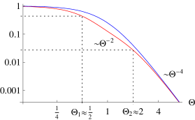
Figure 10: Log-log plot of the dipole bremsstrahlung angular distribution in an isotropic target. Lower (red) curve – semi-classical limit $J_{\mathrm{BH}}\left(0,\Theta\right)/J_{\mathrm{BH}}\left(0,0\right)$. Upper (blue) curve – hard limit $J_{\mathrm{BH}}\left(1,\Theta\right)/J_{\mathrm{BH}}\left(1,0\right)$, equal to the differential intensity pre-factor $1/(1+\Theta^{2})^{2}$. The soft radiation angular distribution exhibits two “knees”, at $\Theta\approx\frac{1}{2}$ and $\Theta\approx 2$ whereas the hard radiation only has one, at $\Theta\approx 1$.

“Double-knee” in the angular distribution of soft radiation.

The function

$$\frac{1+\Theta^{4}}{\left(1+\Theta^{2}\right)^{2}}\equiv 1-\frac{2\Theta^{2}}{\left(1+\Theta^{2}\right)^{2}},$$ (123)

determining at small $x_{\omega}$ the r.h.s. of Eq. (V.2.3), has a minimum at $\Theta=1$ (precisely where the dips in the non-averaged $dW_{\text{dip}}/d\Gamma_{k}$ are located, see Fig. 2). However, function $J_{\mathrm{BH}}\left(0,\Theta\right)$, in fact, does not develop any minimum or shoulder about this point, because it involves yet a pre-factor $1/(1+\Theta^{2})^{2}$ decreasing steeper than (123) rises after its minimum. Nevertheless, some imprint of function (123) remains in behavior of the Bethe-Heitler radiation angular distribution. To show that, let us plot logarithm of $J_{\mathrm{BH}}\left(0,\Theta\right)$ vs. the logarithm of $\Theta$ ($x_{\omega}\approx 0$ is taken to enhance the relative contribution of (123)). In such kind of a plot linear dependence corresponds to a power-law falloff. As compared with the behavior of the pre-factor $1/(1+\Theta^{2})^{2}$, which has on this plot only one “knee” at $\Theta\approx 1$, $J_{\mathrm{BH}}(0,\Theta)$ apparently has two “knees” – at about $\Theta_{1}\approx 0.5$ and at $\Theta_{2}\approx 2$. In between of those two “knees” the behavior is close to $\sim\Theta^{-2}$. Beyond $\Theta_{2}$, the falloff power turns to $\sim\Theta^{-4}$, as is required by the quasi-Rutherford law mentioned in Sec. II.3. This 2-knee shape of the radiation angular distribution may be worth minding at poor statistics measurements, since at the second knee the differential cross-section is already down by a factor of nearly $10^{-2}$. But as $x_{\omega}$ grows, the distribution approaches the 1-knee limiting form.

Polarization maximum and its non-dipole destruction.

For what concerns polarization (shown in Fig. 9(c)), again, the prominent feature is that it reaches 100% at $x_{\omega}\ll 1$, $\Theta=1$, for the reasons already explained (but the example at $\bm{N}=0$ is just the most spectacular). However, with the account of non-dipole effects (see, e. g., May ), polarization in the region $\Theta\approx 1$ must deplete, because, at a definite but large $\hat{\bm{q}}_{\perp}$ the polarization tangential curves are still circles, but their centres are shifted by a vector $\frac{\bm{q}_{\perp}}{2m}$, and none of them coincides with the origin anymore.

VI Summary

The present study suggests that there must exist macroscopic targets, on which relativistic electron scattering, and hence the accompanying forward radiation, possesses a high degree of azimuthal anisotropy. Suitable examples are single crystals oriented by one of their strong crystallographic axes at moderately small orientation angles $\sim 10^{-1}\div 10^{-2}\text{rad}$ with respect to the electron beam direction. The azimuthal anisotropy of the scattering is quantified by parameter $\bm{N}$ introduced in Sec. III. As we have investigated, the azimuthal anisotropy is partially spoiled by nuclei vicinities and by the radiation recoil (see Eq. (86)), but nonetheless, values $N^{2}\geq 0.5$ look realistic.

A straightforward application of polarized bremsstrahlung is for preparation of polarized photon beams (of continuous spectrum). Actually, there is a number of options for extracting polarized photons from the bremsstrahlung flux:

(i) If only isotropic targets are at disposal, there is no alternative to the traditional method Taylor-Mozley of collimating the bremsstrahlung photon flux around the angle $\Theta=1$, i. e., $\theta=1\cdot\gamma^{-1}$.

(ii) If the use of absorber collimators is prohibitive due to radiation angle smallness, as it tends to be at $\gamma>10^{4}$, one needs an intrinsically anisotropic target, the aggregate (naturally narrow) cone of photons emitted on which is polarized. But its polarization degree, according to Eq. (99b), is $\leq N^{2}/2$, with $N^{2}<1$. For efficiency of such a polarized beam, it is desirable to have $N^{2}$ at least $\sim 0.7\div 0.8$.

(iii) Ultimately, if both a collimation tool and an intrinsically anisotropic target are available, one may either look for the highest polarization degree, isolating one of the two spots of enhanced polarization (see Fig. 8). Or, if moderate polarization degree is acceptable provided the beam intensity is high, there is an option of collimating out the strip of angles perpendicular to $\bm{N}$, in between of the polarization zeroes.

Another application of polarized bremsstrahlung from relativistic electrons is for measuring intrinsic anisotropy of the medium the electrons move in. Such kind of diagnostics may be useful during various experiments on relativistic electron interaction with crystal-based targets. Obviously, the radiation leaving the target without much rescattering is better suited for detection than the emitting electrons themselves. Again, for measurement of $\bm{N}$ by the bremsstrahlung yield one can employ a number of techniques:

(i) If the radiation angles can not be resolved, one has to measure $\mathtt{P}_{\text{net}}\propto\frac{N^{2}}{2}$ (Eq. (99b), Fig. 6).

(ii) If the radiation angles are resolvable, one can estimate $\bm{N}$ by the bremsstrahlung intensity azimuthal anisotropy, not employing the polarization detection (Eq. (V), Fig. 2).

(iii) For a finest measurement of $N$, particularly under conditions when it is close to 0 or 1, one can use the method of finding polarization zero locations in the angular distribution (Fig. 8). For $N$ small, it is convenient to measure $\Theta_{<}$, since it is linear in $N$, whereas for $N\to 1$ – the gap $\Theta_{>}-\Theta_{<}$, which is $\sim\sqrt{1-N^{2}}$ (see Sec. V.2.2).

In conclusion, let us yet draw attention to a useful methodic notion – the stereographic projection relation between the laboratory frame and the initial electron rest frame (Sec. II.4). It helps revealing various symmetry properties of relativistic particle bremsstrahlung angular distributions, and may facilitate calculation of bremsstrahlung characteristics in some cases. It must also survive in the non-dipole bremsstrahlung case, which we hope to investigate elsewhere.

Acknowledgements

The author wishes to thank N. P. Merenkov and A. V. Shchagin for useful discussions.

References

- (1) Proceedings of Int. Workshop on Physics with GeV electrons and gamma-rays, 2001, edited by T. Tamae et al. (Tokyo, Universal Acad. Press, 2001) (Also in: Frontiers science series. No. 36).
- (2) M. L. McConnell, J. M. Ryan, D. M. Smith, R. P. Lin, and A. G. Emslie, arXiv:astro-ph/0209384.
- (3) F. Rambo et al., Phys. Rev. C 58, 489 (1998); N. Cabibbo, Phys. Rev. Lett. 7, 386 (1961).
- (4) K. Kirsebom et al., Phys. Lett. B 459, 347 (1999); A. Apyan et al., Phys. Rev. ST-AB 11, 041001 (2008).
- (5) D. S. Gemmel, Rev. Mod. Phys. 46, 129 (1974); V. V. Beloshitsky and F. F. Komarov. Phys. Rep. 93, 117 (1982).
- (6) G. Diambrini Palazzi, Rev. Mod. Phys. 40, 611 (1968).
- (7) M. L. Ter-Mikaelian, High-Energy Electromagnetic Processes in Condensed Media (Wiley-Interscience, N.Y., 1972).
- (8) E. Fermi, Z. Phys. 29, 315 (1924); C. F. Weizsäcker, Z. Phys. 88, 612 (1933); E. J. Williams, Proc. Roy. Soc. 139, 163 (1933); Phys. Rev. 45, 729 (1934).
- (9) C. A. Bertulani and G. Baur, Phys. Rep. 161, 299 (1986).
- (10) V. N. Baier, V. M. Katkov, and V. M. Strakhovenko, Electromagnetic processes at high energies in oriented crystals (World Scientific, Singapore, 1998).
- (11) H. Cheng and T. T. Wu. Expanding Protons: Scattering at High Energies (M.I.T. Press, Cambridge, MA, 1987).
- (12) H. Olsen, L. C. Maximon, and H. Wergeland, Phys. Rev. 106, 27 (1957); V. N. Baier and V. M. Katkov, Sov. Phys. JETP 28, 807 (1968); 28, 854 (1968); A. I. Akhiezer, V. F. Boldyshev, and N. F. Shul’ga, Yad. Fiz. 22, 1185 (1975).
- (13) V. B. Berestetskii, E. M. Lifshitz, and L. P. Pitaevskii, Quantum Electrodynamics (Pergamon-Press, Oxford, 1982).
- (14) O. Klein and Y. Nishina, Z. Phys. 52, 853 (1929).
- (15) V. M. Budnev, I. F. Ginzburg, G. V. Meledin, and V. G. Serbo, Phys. Rep. 15, 181 (1975).
- (16) D. F. Alferov, Yu. A. Bashmakov, and P. A. Cherenkov, Sov. Phys. Usp. 32, 200 (1989).
- (17) B. A. Rosenfeld and N. D. Sergeeva, Stereographic projection (Mir, Moscow, 1977).
- (18) G. Alberi and G. Goggi, Phys. Rep. 74, 1 (1981); N. V. Bondarenko and N. F. Shul’ga, Phys. Lett. B 427, 114 (1998).
- (19) U. Uggerhøj, Rev. Mod. Phys. 77, 1131 (2005).
- (20) M. V. Bondarenco, Phys. Rev. A 81, 052903 (2010).
- (21) R. E. Taylor and R. F. Mozley, Phys. Rev. 117, 835 (1960).
- (22) H. Uberall, Phys. Rev. 107, 223 (1957).
- (23) M. M. May and G. C. Wick, Phys. Rev. 81, 628 (1951); R. L. Gluckstern, M. H. Hull, and G. Breit, Phys. Rev. 90, 1026 (1953); H. Olsen and L. C. Maximon, Phys. Rev. 114, 887 (1959).
- (24) M. M. May, Phys. Rev. 84, 265 (1951).