Density of first Poincaré returns, periodic orbits, and Kolmogorov-Sinai entropy

Abstract.

It is known that unstable periodic orbits of a given map give information about the natural measure of a chaotic attractor. In this work we show how these orbits can be used to calculate the density function of the first Poincaré returns. The close relation between periodic orbits and the Poincaré returns allows for estimates of relevant quantities in dynamical systems, as the Kolmogorov-Sinai entropy, in terms of this density function. Since return times can be trivially observed and measured, our approach to calculate this entropy is highly oriented to the treatment of experimental systems. We also develop a method for the numerical computation of unstable periodic orbits.

1. Introduction

Knowing how often a dynamical system returns to some place in phase space is fundamental to understand dynamics. There is a well established way to quantify that: the first Poincaré return (FPR), which measures how much time a trajectory of a dynamical system takes to make two consecutive returns to a given region. Due to their stochastic behaviour, given a return time it is not feasible to predict the future return times and for that reason one is usually interested in calculating the frequency with which the Poincaré returns happen, the density of the first Poncaré returns (DFP).

This work explains the existence of a strong relationship between unstable periodic orbits (UPOs) and the first Poincaré returns in chaotic attractors. Unstable orbits and first Poincaré returns have been usually employed as a tool to analyse and characterise dynamical systems. With our novel approach we can calculate how frequently returns happen by knowing only a few unstable periodic orbits. Additionally, such relation allows us to easily estimate other fundamental quantities of dynamical systems such as the Kolmogorov-Sinai entropy.

Our motivation to search for a theoretical and simple way of calculating the distribution of Poincaré return times comes from the fact that they can be simply and quickly accessible in experiments and also due to the wide range of complex systems that can be characterized by such a distribution. Among many examples, in Ref. [1] the return times were used to characterize a experimental chaotic laser, in Refs. [2, 3] they were used to characterize extreme events, in Refs. [4, 5] they were used to characterize fluctuations in fusion plasmas, and in Ref. [6] a series of application to complex data analysis were described.

In addition, relevant quantifiers of low-dimensional chaotic systems may be obtained by the statistical properties of the FPR such as the dimensions and Lyapunov exponents [7, 8] and the extreme value laws [9]. For most of the rigorous results concerning the FPR, in particular the form of the DFP [10], one needs to consider very long returns to arbitrarily small regions in phase space, a condition that imposes limitations into the real application to data sets.

We first show how the DFP can be calculated from only a few UPOs inside a finite region. Then, we explain how the DFP can be used to calculate quantities as the Kolmogorov-Sinai entropy, even when only short return times are measured in finite regions of the phase space.

Our work is organized as follows: We first introduce the work of Ref. [11], which relates the natural measure of a chaotic attractor to the UPOs embedded in a chaotic attractor. The measure of a chaotic attractor refers to the frequency of visits that a trajectory makes to a portion of the phase space. This measure is called natural when it is invariant for typical initial conditions. This appears in Sec. 2, along with the relevant definitions. In Sec. 3 we define $\rho(\tau,S)$ the density of first Poincaré returns for a time $\tau$ to a subset $S$ of phase space and we study the relation between the UPOs and this function. This can be better understood if we classify the UPOs inside $S$ as recurrent and non-recurrent. Recurrent are those UPOs that return more than once to the subset $S$ before completing its cycle. Non-recurrent are UPOs that visits the subset $S$ only once in a period. While in the calculation of the natural measure of $S$ one should consider the two types of UPOs with a given large period inside it, for the calculation of the DFP for a time $\tau$ one should consider only non-recurrent UPOs with a period $\tau$. Sec. 4 is mostly dedicated to show how to calculate $\rho(\tau,S)$ even when not all non-recurrent UPOs of a large period are known. Such a situation typically arises when the time $\tau$ is large. We have numerically shown that the error of our estimation becomes smaller, the longer the period of the UPOs and the larger the number of UPOs considered.

Throughout the paper we illustrate results by presenting the calculations for the tent map. Finally, in Sec. 6 we show numerical results on the logistic map that support our approach. In particular, we obtain numerical estimates of the Kolmogorov-Sinai entropy, the most successful invariant in dynamics, so far. The estimates are obtained considering the density of only short first return times, as discussed in Sec. 5. The UPOs of period $p$ are computed numerically as stable periodic orbits of a system of $p$ coupled cells, a method described in 6.5.

2. Definitions and results

Consider a d-dimensional $C^{2}$ map of the form $x_{n+1}=F(x_{n})$, where $x\in\Omega\subset R^{d}$ and $\Omega$ represents the phase space of the system. Consider $A\subset\Omega$ to represent a chaotic attractor. By chaotic attractor we mean an attractor that has at least one positive Lyapunov exponent.

For a subset $S$ of the phase space and an initial condition $x_{0}$ in the basin of attraction of $A$, we define $\mu(x_{0},S)$ as the fraction of time the trajectory originating at $x_{0}$ spends in $S$ in the limit that the length of the trajectory goes to infinity. So,

(1) $$\mu(x_{0},S)=\lim_{n\rightarrow\infty}\frac{\sharp\{F^{i}(x_{0})\in S,\ 0\leq i\leq n\}}{n}.$$

Definition 2.1.

If $\mu(x_{0},S)$ has the same value for almost every $x_{0}$ (with respect to the Lebesgue measure) in the basin of attraction of $A$, then we call the value $\mu(S)$ the natural measure of $S$.

For now we assume that our chaotic attractor $A$ has always a natural measure associated to it, normalized to have $\mu(A)=1$. In particular this means that the attractor is ergodic[11].

We also assume that the chaotic attractor $A$ is mixing: given two subsets, $B_{1}$ and $B_{2}$, in $A$, we have:

$$\lim_{n\rightarrow\infty}\mu(B_{1}\cap F^{-n}(B_{2}))=\mu(B_{1})\mu(B_{2}).$$

In addition, we consider $A$ to be a hyperbolic set.

The eigenvalues of the Jacobian matrix of the $n$-th iterate, $F^{n}$, at the $j$th fixed point $x_{j}$ of $F^{n}$ are denoted by $\lambda_{1j},\lambda_{2j},...,\lambda_{uj},\lambda_{(u+1)j},...,\lambda_{dj}$, where we order the eigenvalues from the biggest, in magnitude, to the lowest and the number of the unstable eigenvalues is $u$. Let $L_{j}(n)$ be the product of absolute values of the unstable eigenvalues at $x_{j}$.

Then it was proved by Bowen in 1972 [12] and also by Grebogi, Ott and Yorke in 1988 [11] the following:

Theorem 2.1.

For mixing hyperbolic chaotic attractors, the natural probability measure of some closed subset $S$ of the d-dimensional phase space is

(2) $$\mu(S)=\lim_{n\rightarrow\infty}\sum_{x_{j}}L^{-1}_{j}(n),$$

where the summation is taken over all the fixed points $x_{j}\in S$ of $F^{n}$.

This formula is the representation of the natural measure in terms of the periodic orbits embedded in the chaotic attractor. To illustrate how it works let us take a simple example like the tent map:

Example 2.1.

Let us consider $F:[0,1]\rightarrow[0,1]$ such that

$$F(x)=\left\{\begin{array}[]{l}2x,\ if\ x\in[0,1/2]\\ 2-2x,\ if\ x\in]1/2,1]\end{array}\right.$$

For this map there is only one unstable direction. Since the absolute value of the derivative is constant in $[0,1]$ we have $L_{j}(\tau)=L(\tau)=2^{\tau}$.

For the tent map, periodic points are uniformly distributed in $[0,1]$. Using this fact together with some of the ideas of G.H. Gunaratne and I. Procaccia [13], it is reasonable to write the natural measure of a subset $S$ of $[0,1]$ as:

(3) $$\mu(S)=\lim_{\tau\rightarrow\infty}\frac{N(\tau,S)}{N(\tau)},$$

where $N(\tau,S)$ is the number of fixed points of $F^{\tau}$ in $S$ and $N(\tau)$ is the number of fixed points of $F^{\tau}$ in all space $[0,1]$. For this particular case we have $N(\tau)=L(\tau)=L_{j}(\tau)$ and so

$$\mu(S)=\lim_{\tau\rightarrow\infty}\frac{N(\tau,S)}{N(\tau)}=\lim_{\tau\rightarrow\infty}\frac{N(\tau,S)}{L(\tau)}=\lim_{\tau\rightarrow\infty}\sum_{j=1}^{N(\tau,S)}\frac{1}{L_{j}(\tau)}$$

and we obtain the Grebogi, Ott and Yorke formula.

3. Density of first returns and UPOs

In this section we relate the DFP, $\rho(\tau,S)$, and the UPOs of a chaotic attractor. We show in Eq. (10) that $\rho(\tau,S)$ can also be calculated in terms of the UPOs but one should consider in Eq. (2) only the non-recurrent ones.

3.1. First Poincaré returns

Consider a map $F$ that generates a chaotic attractor $A\subset\Omega$, where $\Omega$ is the phase space. The first Poincaré return for a given subset $S\subset\Omega$ such that $S\cap A\neq\emptyset$ is defined as follows.

Definition 3.1.

A natural number $\tau$, $\tau>0$, is the first Poincaré return to $S$ of a point $x_{0}\in S$ if $F^{\tau}(x_{0})\in S$ and there is no other $\tau^{*}<\tau$ such that $F^{\tau^{*}}(x_{0})\in S$.

A trajectory generates an infinite sequence, $\tau_{1},\tau_{2},...,\tau_{i}$, of first returns where $\tau_{1}=\tau$ and $\tau_{i}$ is the first Poincaré return of $F^{n_{i}}(x_{0})$ with $n_{i}=\sum_{n=1}^{i-1}\tau_{n}$.

The subset $S^{\prime}$ of points in $S\subset\Omega$ that produce FPRs of length $\tau$ to $S$ is given by

(4) $$S^{\prime}=S^{\prime}(\tau,S)=\left(F^{-\tau}(S)\cap S\right)-\bigcup_{0<j<\tau}\left(F^{-j}(S)\cap S\right).$$

3.2. Density function

In this work, we are concerned with systems for which the DFP decreases exponentially as the length of the return time goes to infinity. Such systems have mixing properties and as a consequence we expect to find $\rho(\tau,S)\approx\mu(S)(1-\mu(S))^{\tau-1}$, where $(1-\mu(S))^{\tau-1}$ represents the probability of a trajectory remaining $\tau-1$ iterations out of the subset $S$. We are interested in systems for which the decay of $\rho(\tau)$ is exponential, i.e., $\rho(\tau)\propto e^{-\alpha\tau}$.

The usual way of defining $\rho(\tau,S)$, for a given subset $S\subset\Omega$, is by measuring the fraction of returns to $S$ that happen with a given length $\tau$ with respect to all other possible first returns [see Eq. (27)]. It is usually required for a density that

$$\int\rho(\tau,S)d\tau=1.$$

In this work, we also adopt a more appropriate definition for $\rho(\tau,S)$ in terms of the natural measure. We define the function $\rho(\tau,S)$ as the natural measure of the set of orbits that makes a first return $\tau$ to $S$ divided by the natural measure in $S$. More rigorously, we have:

Definition 3.2.

The density function of the first Poincaré return $\tau$ for a particular subset $S\subset\Omega$ such that $\mu(S)\neq 0$ is defined as

(5) $$\rho(\tau,S)=\frac{\mu(S^{\prime})}{\mu(S)},$$

where $S^{\prime}=S^{\prime}(\tau,S)\subset S$ is the subset of points that produce FPRs of length $\tau$ defined in Eq. (4).

Even for a simple dynamical system as the tent map, the analytical calculation of $\rho(\tau,S)$ is not trivial. However, an upper bound for this function can be easily derived as in the following example:

Example 3.1.

Consider the tent map defined in example 2.1, for which the natural measure coincides with the Lebesgue measure $\lambda$, and let $S\subset[0,1]$ be a non-trivial closed interval.

To have a return to $S$ we only need to know the natural number $n^{*}$ such that $F^{n^{*}}(S)=[0,1]$. Since $F$ is an expansion, this natural number always exists. To find it when $\lambda(S)=\epsilon>0$, we first solve the equation $2^{x^{*}}={1}/{\epsilon}$ and get $x^{*}={-\log(\epsilon)}/{\log(2)}$, so we take $n^{*}=\left[{-\log(\epsilon)}/{\log(2)}\right]+1$, where $[x]$ represents the integer part of $x$. Then $n^{*}$ is an upper bound for $\tau_{min}$, the shortest first return to $S$.

Most intervals $S$ of small measure have large values of $\tau_{min}$ and $\tau_{min}\approx n^{*}$ is a good approximation. A sharper upper bound for $\tau_{min}$ in $S$ is the lowest period of an UPO that visits it.

The set $D=F^{-n^{*}}(S)\cap S\neq\emptyset$ represents the fraction of points in $S$ that return to $S$ (not necessarily first return) after $n^{*}$ iterations. Using Eq. (5) and since $S^{\prime}\subset D$ we have

$$\rho(n^{*},S)\leq\frac{\lambda(D)}{\lambda(S)}\leq\frac{\epsilon\frac{1}{2^{n^{*}}}}{\epsilon}=2^{-n^{*}}.$$

It is natural to expect that for $\tau$ of the order of $n^{*}$ and close to $\tau_{min}$ we have $\rho(\tau,S)\leq 2^{-\tau}$.

We can write this equation as $\rho(\tau,S)\leq e^{(-\tau\log(2))}=e^{(-\tau\lambda_{1})}$, where $\lambda_{1}=\log(2)$ is the Lyapunov exponent for the tent map. In fact, in 1991, G. M. Zaslavsky and M. K. Tippett

[14][15] presented one formula for the exact value of

$\rho(\tau,S)$. That result can only be valid under the same conditions that we have used previously, i.e. $\tau\approx\tau_{min}$ and for most sets of sufficiently small measure $\epsilon$, so that $\tau_{min}\approx n^{*}$.

3.3. Density function in terms of recurrent and non-recurrent UPOs

Since our chaotic attractor $A$ is mixing, the natural measure associated with $A$ satisfies, for any subset $S$ of nonzero measure:

$$\mu(S)=\lim_{\tau\rightarrow\infty}\frac{\mu(S\cap F^{-\tau}(S))}{\mu(S)}.$$

We can write the right hand side of the last equation, for any positive $\tau$, in two terms:

(6) $$\frac{\mu(S\cap F^{-\tau}(S))}{\mu(S)}=\frac{\mu(S^{\prime})}{\mu(S)}+\frac{\mu(S^{*})}{\mu(S)}$$

with $S^{\prime}$ as defined in Eq. (4) and where $S^{*}=S^{*}(S,\tau)$ is the set of points in $S$ that are mapped to $S$ after $\tau$ iterations but for which $\tau$ is not the FPR to $S$, so $S^{\prime}\cup S^{*}=(S\cap F^{-\tau}(S))$ and $S^{\prime}\cap S^{*}=\emptyset$.

An UPO of period $\tau$ is recurrent with respect to a set $S\subset\Omega$ if there is a point $x_{0}\in S$ in the UPO with $F^{n}(x_{0})\in S$ for $0<n<\tau$. In other words, its FPR is less than its period. Thus, the UPOs in the set $S^{*}$ are all recurrent. We refer to them as the recurrent UPOs inside $S$.

Associated with the recurrent UPOs in $S$ we define

(7) $$\mu_{R}(\tau,S)=\sum_{j}\frac{1}{L_{j}^{R}(\tau)}$$

and associated with the non-recurrent UPOs in $S$ we define

(8) $$\mu_{NR}(\tau,S)=\sum_{j}\frac{1}{L_{j}^{NR}(\tau)}$$

where $L_{j}^{R}(\tau)$ and $L_{j}^{NR}(\tau)$ refer, respectively, to the product of the absolute values of the unstable eigenvalues of recurrent and non-recurrent UPOs of period $\tau$ that visit $S$.

Notice that, if $\mu(S)\neq 0$,

$$\lim_{\tau\rightarrow\infty}\frac{\mu(S^{*})}{\mu(S)}=\lim_{\tau\rightarrow\infty}\mu_{R}(\tau,S)$$

and

(9) $$\lim_{\tau\rightarrow\infty}\frac{\mu(S^{\prime})}{\mu(S)}=\lim_{\tau\rightarrow\infty}\mu_{NR}(\tau,S)$$

since $\mu(S^{*})/\mu(S)$ measures the frequency with which chaotic trajectories that are associated with the recurrent UPOs visit $S$ and $\mu(S^{\prime})/\mu(S)$ measures the frequency with which chaotic trajectories that are associated with the non-recurrent UPOs visit $S$.

Comparing Eqs. (5), (6) and (9) we obtain the following:

Main Idea: For a chaotic attractor $A$ generated by a mixing uniformly hyperbolic map $F$, for a small subset $S\subset A$, generated by a Markov partition and such that the measure in $S$ is provided by the UPOs inside it, we have that

(10) $$\rho(\tau,S)\approx\mu_{NR}(\tau,S),$$

for a sufficiently large $\tau$. Moreover,

$$\mu(S)=\lim_{\tau\rightarrow\infty}[\rho(\tau,S)+\mu_{R}(\tau,S)].$$

A Markov partition is a very special splitting of the phase space. For the purpose of better justifying Eq. (10), if a region $C(\tau)$ belongs to a Markov partition of order $\tau$, then there is a sub-interval $\tilde{C}(\tau)$ of $C(\tau)$ that after $\tau$ iterations is mapped exactly over $C(\tau)$. Moreover, points inside $\tilde{C}(\tau)$ make first returns to $C(\tau)$ after $\tau$ iterations. Then, $\mu_{R}(\tau,C(\tau))$=0. As a consequence, for sufficiently large $\tau$ we can write that $\mu[C(\tau)]\rightarrow\rho[\tau,C(\tau)]$.

But approximation (10) remains valid for a small nonzero $\tau$. The reason for that is the following: Notice that from the way Kac’s lemma is derived (see Sec. 8.1), Eq. (2) can be written as

$$\mu(S)=\frac{\int_{\tau_{min}}^{\infty}\rho(\tau,S)d\tau}{<\tau>},$$

where $<\tau>$ represents the average of the FPRs inside $S$, since $\int_{\tau_{min}}^{\infty}\rho(\tau,S)d\tau=1$. This equation illustrates that any possible existing error in the calculation of $\mu(S)$ by Eq. (2) is a summation over all errors coming from $\rho(\tau,S)$ for all values of $\tau$ that we are considering. As shown in Ref. [11], $\mu(S)$ can be calculated by Eq. (2) using UPOs with a small and finite period $p$. This period is of the order of the time that the Perron-Frobenius operator converges and thus linearization around UPOs can be used to calculate the measure associated with them. As a consequence, if $\mu(S)$ can be well estimated for $p\approx 30$ then $\rho(\tau,S)$ can be well estimated for $\tau<<p$. As we will observe, considering $\tau$ small, of the order of $5$, we get a very good estimation for $\rho(\tau,S)$.

In addition, we observe in our numerical simulation that $S$ does not need to be a cell in a Markov partition but just a small region located in an arbitrary location in $\Omega$.

We say that an UPO has FPRs associated with it if the UPO is non-recurrent. See that for every UPO there is a neighborhood containing no other UPO with the same period. If the UPO is non-recurrent then all points inside a smaller neighborhood will produce FPRs associated with this UPO in the sense that their FPR coincides with the UPO’s. Consider $\tau_{min}$ as the shortest first return in $S$.

Case $\tau<2\tau_{min}$

UPOs of period $\tau$ are non-recurrent. This is illustrated in Fig. 1 (A), where $\tau_{min}=7$, for the logistic map ($c=4$). In that picture we observe that for $\tau\leq 14$ all FPRs are associated with UPOs. Because of this fact $\mu(S^{*})=0$ and then all the chaotic trajectories that return to $S$ are associated with non-recurrent UPOs. So, $\rho(\tau,S)\approx\mu(S)$ and thus, $\rho(\tau,S)\approx\mu_{NR}(\tau,S)$.

Case $\tau\geq 2\tau_{min}$

We can have recurrent UPOs of period $\tau$, that do not have first returns associated with them. As a consequence $\mu(S^{*})>0$ and recurrent UPOs contribute to the measure of $S$. This is illustrated in Fig. 1 (B), when $\tau=16$.

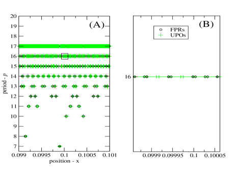
Figure 1. This picture shows some UPOs inside $S\subset[0,1]$ and first Poincaré returns for the logistic map, [$x_{n+1}=4x_{n}(1-x_{n})$]. In this example $\tau_{min}=7$. For $\tau<14$ all UPOs have FPRs associated with them. For $\tau\geq 14$ (as in (B) for $\tau=16$) some UPOs are recurrent. Picture (B) is a zoom of picture (A).

4. How to calculate the density of first Poincaré returns

A practical issue is how to calculate $\mu_{NR}(\tau,S)$. There are two relevant cases: All UPOs can be calculated; only a few can be calculated.

Assuming $\tau$ to be sufficiently small such that all UPOs of period $\tau$ can be calculated and sufficiently large so that Eq. (10) is reasonably valid, $\mu_{NR}(\tau,S)$ can be exactly calculated and we can easily estimate $\rho(\tau,S)$ from Eq.(10), using $\rho(\tau,S)\approx\mu_{NR}(\tau,S)$.

When $\tau$ is large then, typically, only a few UPOs can be calculated. For this case, it is difficult to use Eq. (10) to estimate $\rho(\tau,S)$ since there will be too many UPOs. In order to calculate $\rho(\tau,S)$ using $\mu_{NR}(\tau,S)$ we do the following. First notice that

(11) $$\mu(S)=\lim_{\tau\rightarrow\infty}(\mu_{NR}(\tau,S)+\mu_{R}(\tau,S)).$$

Considering then $\tau$ sufficiently large we have that

$$\mu(S)\approx\mu_{NR}(\tau,S)+\mu_{R}(\tau,S)$$

which can be rewritten (using Eq. (10) which says that $\rho(\tau,S)\approx\mu_{NR}(\tau,S)$, for finite $\tau$] as

(12) $$\rho(\tau,S)\approx\mu(S)-\mu_{R}(\tau,S)=\mu(S)\left(1-\frac{\mu_{R}(\tau,S)}{\mu(S)}\right).$$

This equation allows us to reproduce, approximately, the function $\rho(\tau,S)$, for any sufficiently large $\tau$, only using the estimated value of the quotient

$$\frac{\mu_{R}(\tau,S)}{\mu(S)}$$

that is easy to obtain numerically, since not all UPOs should be calculated but just a few ones with period $\tau$. We discuss this in 4.1 below.

4.1. How can we estimate $\mu_{R}(\tau,S)/\mu(S)$?

Considering a subset $S$ and fixing $\tau$, we calculate a number $t$ of different UPOs with period $\tau$ (say, $t=50$) inside $S$ (It is explained in Sec. 6.5 how to calculate numerically UPOs with any period of a given map). These UPOs are calculated from randomly selected symbolic sequences for which the generated UPOs visit $S$. See that, for example, in the tent map, for $\tau=10$ and $S=[0,\frac{1}{8}]$, we may have $2^{10}/8$ UPOs inside $S$ and so, here $50$ UPOs inside $S$ is, in fact, a very small number of UPOs.

Now, we separate all the $t$ UPOs that visit $S$ into recurrent and non-recurrent ones and suppose that we have $r$ recurrent and $nr$ non-recurrent such that $r+nr=t$. So, $r$ and $nr$ depend on $t$ and $S$. With these particular $r(t,S)$ recurrent UPOs we use Eq. (7) and we obtain

$$\tilde{\mu}_{R}[\tau,S,r(t,S)]=\sum_{j=1}^{r(t,S)}\frac{1}{L_{j}^{R}(\tau)}$$

where $L_{j}^{R}(\tau)$ represents the product of the absolute values of the unstable eigenvalues of the $j$th recurrent UPO within the set of $r(t,S)$ recurrent UPOs. See that this quantity is not equal to $\mu_{R}(\tau,S)$ since we are not considering all recurrent UPOs inside $S$ but just a small number $r(t,S)$ of them. We do the same thing with the $nr(t,S)$ non-recurrent UPOs and obtain the quantity $\tilde{\mu}_{NR}[\tau,S,nr(t,S)]$.

Finally, we observe that, for a sufficiently large $t$, we have

$$\frac{\tilde{\mu}_{R}[\tau,S,r(t,S)]}{\tilde{\mu}(\tau,S,t)}\approx\frac{\mu_{R}(\tau,S)}{\mu(S)},$$

where $\tilde{\mu}(\tau,S,t)=\tilde{\mu}_{R}[\tau,S,r(t,S)]+\tilde{\mu}_{NR}[\tau,S,nr(t,S)]$. Therefore, with only a few UPOs inside $S$ we calculate an estimated value for $\rho(\tau,S)$. This estimation is represented by $\rho_{M}$ and is given by

(13) $${\rho}_{M}[\tau,S,r(t,S)]=\mu(S)\left(1-\frac{\tilde{\mu}_{R}[\tau,S,r(t,S)]}{\tilde{\mu}(\tau,S,t)}\right)$$

Notice that, for a large $\tau$ we will have more recurrent UPOs than non-recurrent ones and therefore the larger $\tau$ is, the larger is the contribution of the recurrent UPOs to the measure inside $S$.

4.2. Error in the estimation

To study how much our estimation in Eq. (13) depends on the number $t$ of UPOs, we first assume that if all UPOs are known, the calculated distribution in Eq. (10) is “exact”, or in other words it has a neglectable error as when compared to the real distribution provided by Eq. (5).

Then, the error in Eq. (13) will depend on the deviation of the quotient

(14) $$q_{1}=\frac{\tilde{\mu}_{R}[\tau,S,r(t,S)]}{\tilde{\mu}(\tau,S,t)},$$

calculated when only $t$ UPOs are known, to the quotient

(15) $$q_{2}=\frac{\tilde{\mu}_{R}[\tau,S,r(t=N(\tau,S),S)]}{\tilde{\mu}(\tau,S,t=N(\tau,S))},$$

calculated when all the $N(\tau,S)$ UPOs are known.

Thus, the amount of error that our estimate [Eq. (13)] has as when compared to the “exact” value of $\rho$ (when all the UPOs are known) can be calculated by

(16) $$E[\tau,S,t]=\frac{|q_{1}-q_{2}|}{q_{2}}$$

which means that the quantity $E$ gives the amount of deviation, in a scale from 0 to 1, of $\rho_{M}$ [Eq. (13)] as when compared to the “exact” value of $\rho$ [Eq. (10)]. Notice that in Eq. (16), the quantity 100$E$ corresponds to the percentage of error that our estimation has.

4.3. Uniformly distributed UPOs

There is another way to estimate the value of $\rho(\tau,S)$ in terms of the number of UPOs in a subset $S$ of a chaotic attractor $A$. We define $N(\tau)$ as the number of fixed points of $F^{\tau}$ in $A$, $N(\tau,S)$ as the number of fixed points of $F^{\tau}$ in $S$, $N_{R}(\tau,S)$ as the number of fixed points of $F^{\tau}$ in $S$ whose orbit under $F$ is recurrent and $N_{NR}(\tau,S)$ as the number of fixed points of $F^{\tau}$ in $S$ whose orbit under $F$ is non-recurrent. Then, for a sufficiently large $\tau$ and for a uniformly hyperbolic dynamical system for which periodic points are uniformly distributed in $A$, we have

$$\mu_{R}(\tau,S)\approx\frac{N_{R}(\tau,S)}{N(\tau)},\ \ \mu_{NR}(\tau,S)\approx\frac{N_{NR}(\tau,S)}{N(\tau)}.$$

Using the previous approximations we can write

$$\mu(S)\approx\frac{N_{R}(\tau,S)}{N(\tau)}+\frac{N_{NR}(\tau,S)}{N(\tau)}=\frac{N(\tau,S)}{N(\tau)}.$$

By Eq. (10) we may write $\rho(\tau,S)\approx\mu_{NR}(\tau,S)$ and we have that

(17) $$\rho(\tau,S)\approx\mu(S)-\frac{N_{R}(\tau,S)}{N(\tau)}.$$

which can be written as

(18) $$\rho(\tau,S)\approx\mu(S)\left(1-\frac{N_{R}(\tau,S)}{N(\tau,S)}\right).$$

Again, we have an expression with a quotient

$$\frac{N_{R}(\tau,S)}{N(\tau,S)}$$

that is, again, easy to obtain numerically by the same technique from which $\mu_{R}/\mu$ can be estimated and therefore we can obtain an estimation for $\rho(\tau,S)$, represented by $\rho_{N}$, by

(19) $${\rho}_{N}[\tau,S,r(t,S)]=\mu(S)\left(1-\frac{r(t,S)}{t}\right)$$

where $r(t,S)$ represents the number of recurrent UPOs out of a total of $t$ UPOs, exactly as previously defined.

5. Kolmogorov-Sinai entropy

In 1958 Kolmogorov introduced the concept of entropy into ergodic theory and this has been the most successful invariant so far[16]. In this section we explain how to use the density of first Poincaré returns to estimate the Kolmogorov-Sinai entropy $H_{KS}$.

The exposition here does not aim to be rigorous, only to explain how we have arrived at the numerical estimates for the logistic map of Sec. 6. which is a non-uniformly hyperbolic map.

It is known that[17]

(20) $$N(\tau)\propto\exp(\tau H_{KS}).$$

Consider $F$ as a dynamical system that has the following property:

$$\frac{N_{NR}(\tau,S)}{N(\tau)}\approx\mu_{NR}(\tau,S)\approx\rho(\tau,S),$$

for a sufficiently large $\tau$. For example, dynamical systems for which periodic points are uniformly distributed on the chaotic attractor $A$ have this property.

Considering the tent map and $S\subset[0,1]$ such that $N_{NR}(\tau,S)=1$ (if there is more that one non-recurrent UPO of period $\tau$ inside $S$ we shrink $S$ to have only one), we have $\rho(\tau,S)\approx\frac{1}{2^{\tau}}$ that agrees with example 3.1, for $\tau$ close to $\tau_{min}$ and for most intervals $S$. For other non-uniformly hyperbolic systems as the logistic the Hénon maps, this property holds in an approximate sense and this approximation is better the larger $\tau$ is and the closer the interval $S$ is to a Markov partition.

Using the last approximation together with Eq. (20) we may write

$$\frac{N_{NR}(\tau,S)}{\rho(\tau,S)}\approx b\exp(\tau H_{KS}),$$

for some positive constant $b\in R$. So, we have that

(21) $$H_{KS}\approx\frac{1}{\tau}\log\left(\frac{N_{NR}(\tau,S)}{b\rho(\tau,S)}\right)=\frac{1}{\tau}\log\left(\frac{N_{NR}(\tau,S)}{\rho(\tau,S)}\right)-\frac{\log(b)}{\tau}.$$

We define the quantity $H(\tau,S)$ as

(22) $$H(\tau,S)=\frac{1}{\tau}\log\left(\frac{N_{NR}(\tau,S)}{\rho(\tau,S)}\right)$$

and then, for $b\geq 1$, it is clear that

$$H_{KS}\approx\frac{1}{\tau}\log\left(\frac{N_{NR}(\tau,S)}{b\rho(\tau,S)}\right)\leq H(\tau,S),$$

so $H(\tau,S)$ is a local upper bound for the approximation of $H_{KS}$, considering a sufficiently large $\tau$.

Supposing that there is at least one non-recurrent UPO inside $S$, then for large $\tau$ we have $\frac{N_{NR}(\tau,S)}{\rho(\tau,S)}>\!\!>b$, as $b$ is constant. Thus, the term

$$\frac{1}{\tau}\log\left(\frac{N_{NR}(\tau,S)}{\rho(\tau,S)}\right)$$

dominates the expression (21), for longer times.

This equation allows us to obtain an upper bound for $\rho(\tau,S)$. See that $\rho(\tau,S)\leq N_{NR}(\tau,S)\exp(-\tau H_{KS})$ and if $\tau\approx\tau_{min}$ then $N_{NR}(\tau,S)\approx 1$ and we obtain $\rho(\tau,S)\leq\exp(-\tau H_{KS})$ as in example 3.1.

Equation (22) depends on the choice of the subset $S$ and is then a local estimation for $H_{KS}$. To have a global estimate we take a finite number, $n$, of subsets $S_{i}$ in the chaotic attractor and make a space average as

(23) $$\frac{1}{\tau n}\sum_{i=1}^{n}\log\left(\frac{N_{NR}(\tau,S_{i})}{\rho(\tau,S_{i})}\right).$$

Better results are obtained taking the average over pairwise disjoint subsets $S_{i}$ that are well distributed over $A$.

When we consider $N_{NR}(\tau,S)=1$ this means that we have only one non-recurrent UPO, with period $\tau$, inside $S$. In general, for sufficiently small subsets, $S_{i}$, we may have $N_{NR}(\tau,S_{i})=1\ \forall i$ and we obtain an approximation that only depends on the density function of the first Poincaré returns

(24) $$H_{KS}\approx\frac{1}{\tau n}\sum_{i}\log\left(\frac{1}{\rho(\tau,S_{i})}\right).$$

An equation which can be trivially used from the experimental point of view since we just need to estimate $\rho(\tau,S_{i})$ and we do not need to know the UPOs. For practical purposes, we consider in Eqs. (22), (23) and (24) that $\tau=\tau_{min}$.

6. Numerical results

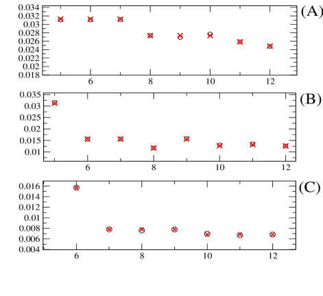
Figure 2. Density function of the FPRs, $\rho(\tau,S)$, as empty circles and the measure of the non-recurrent periodic orbits, $\mu_{NR}(\tau,S)$, as crosses, considering the following intervals: (A), $S=[0.3-0.05,0.3+0.05]$; (B), $S=[0.3-0.01,0.3+0.01]$; (C), $S=[0.3-0.005,0.3+0.005]$.

Figure 3. Red empty circles represent $\rho(\tau,S)$ estimated by Eq. (12), green crosses estimated by Eq. (18) and the black line calculated by Eq. (27). Picture (B) is just a similar reproduction of (A) considering longer first return times. We consider 200 UPOs inside $S=[0.1-0.001,0.1+0.001]$, for each $\tau$.

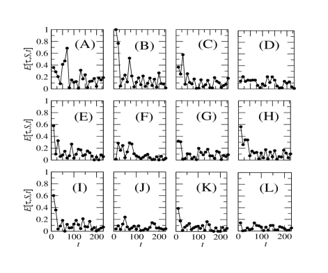
Figure 4. We show the quantity $E[\tau,S,t]$ with respect to the number $t$ of UPOs randomly chosen, for $\tau=9$ (A), $\tau=10$ (B), $\tau=11$ (C), $\tau=12$ (D), $\tau=13$ (E), $\tau=14$ (F), $\tau=15$ (G), $\tau=16$ (H), $\tau=17$ (I), $\tau=18$ (J), $\tau=19$ (K), and $\tau=20$ (L). The quantity $E$ gives the amount of deviation, in a scale from 0 to 1, of $\rho_{M}$ [Eq. (13)] as compared to the “exact” value of $\rho$ [Eq. (10)]. We consider an interval positioned at $x=0.04$ with size $\epsilon=0.02$.

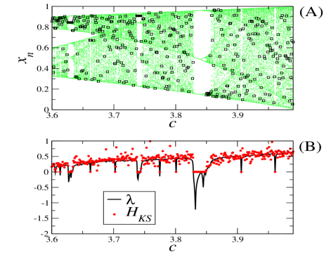
Figure 5. (A) A bifurcation diagram as points (light green) and the randomly chosen intervals as empty (black) squares. (B) Lyapunov exponent as line and filled circles representing the $H_{KS}$ entropy using Eq. (22), for the logistic family. We consider 400 values of $c$ and for each $c$ the size of the set $S$ is $\epsilon=0.002$.

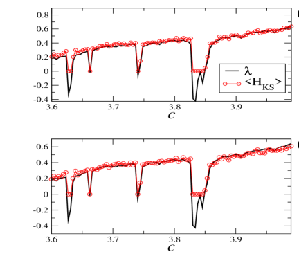
Figure 6. The Lyapunov exponent $\lambda$ as line and the aproximation of $H_{KS}$ entropy using Eqs. (23) and (24) as empty circles. (A), Eq. (23); (B), Eq. (24). In this simulation we consider 100 values of $c$ and for each $c$ we consider $40$ subsets $S_{i}$ each one with lenght $\epsilon=0.002$. A subset $S_{i}$ is picked only if $\tau_{min}\in[10,14]$.

We illustrate our ideas with simulations on the logistic family $F:[0,1]\rightarrow[0,1]$ given by

(25) $$F(x)=cx(1-x),$$

were $c\in R$. There are many biological motivations to study this family of maps[18]. The maps that we obtain when the parameter $c$ is varied have interesting mathematical properties. It is therefore of relevant use for mathematical and biological study. Moreover, for this family it is possible to compare the estimates made using all the UPOs to those using only some UPOs.

For most numerical simulations in this section we take $c=4$ in Eq. (25), for which the map is chaotic and the chaotic attractor is compact.

6.1. Calculating $\rho$ when all UPOs are known

Figure 2 shows the function $\rho(\tau,S)$ calculated by Eq. (27) and the values of $\mu_{NR}(\tau,S)$ calculated by Eq. (8), for some subsets $S$. See that the DFP can be almost exactly obtained if all the non-recurrent UPOs inside $S$ with period $\tau$ can be calculated: In Sec. 3 we concluded that $\rho(\tau,S)\approx\mu_{NR}(\tau,S)$.

6.2. Calculating $\rho$ when not all UPOs are known

Figure 3 shows the approximations for $\rho(\tau,S)$ using Eqs. (13) and (19). In (B), comparing with (A), we consider longer first return times. We only use Eqs. (13) and (19) for $\tau>2\tau_{min}$.

6.3. Error of our estimation when not all UPOs are known

To numerically calculate the error [Eq. (16)] of our estimation in Eq. (13), we only consider UPOs with a period smaller than 20. The reason is because in order to calculate the quotient $q_{2}$ in Eq. (15), all the UPOs must be known. Considering larger periods than 20 would be computationally demanding, even thought the proposed method to calculate UPOs is capable of finding them all.

It is also required that $\tau>2\tau_{min}$, once that to calculate the quotient $q_{1}$ in Eq. (14) there has to exist at least one recurrent UPO within the set of $t$ UPOs considered, i.e. $r\geq 1$. Therefore, we need to choose the size of the interval such that 20-2$\tau_{min}-1$ is sufficiently large, meaning an interval for which $\tau_{min}$ is sufficiently smaller. We have chosen $\epsilon$=0.02.

Since the error of our estimation is proportional to a quotient between two quantities that depend on the number $r$ of recurrent UPOs, it is advisable that one consider intervals for which a reasonable number of recurrent UPOs are found, even when their period is short (smaller or equal than 20). Such interval is positioned in places were the natural measure is large. In the case of the logistic map, these intervals are positioned either close to $x$=0 or $x=1$. Therefore, we consider an interval positioned at $x=0.04$. From the previous considerations, we consider that the interval has a size of $\epsilon=0.02$.

In Fig. 4(A-I), we show the quantity $E[\tau,S,t]$ with respect to the number $t$ of UPOs randomly chosen, for $\tau=9$ (A), $\tau=10$ (B), $\tau=11$ (C), $\tau=12$ (D), $\tau=13$ (E), $\tau=14$ (F), $\tau=15$ (G), $\tau=16$ (H), $\tau=17$ (I), $\tau=18$ (J), $\tau=19$ (K), and $\tau=20$ (L).

The most important information from these figures is that as UPOs of longer periods are considered [going from Fig. (A) to (L)], the error $E$ of our estimation decreases in an average sense considering all the values of $t$. Another relevant point is that the larger the number $t$ of UPOs considered, the smaller the error. Notice that the total number of UPOs of period $\tau$ is given by 2^τ. Therefore, looking at Fig. 4(L), one can see that even considering only about 0.0009$\%$ of all the UPOs (10 UPOs, out of a total of 2²⁰=1048576), the error of our estimation is smaller than $14\%$ when compared to the “exact” value of $\rho$.

6.4. Estimating the KS entropy

In order to know how good our estimation for $H_{KS}$ is we use Pesin’s equality which states that $H_{KS}$ equals the sum of the positive Lyapunov exponents, here denoted by $\lambda$. For the logistic map there is at most one positive Lyapunov exponent.

Figure 5 shows the approximation for the quantity $H_{KS}$ using Eq. (22). See that Eq. (22) only needs one subset $S$ on the chaotic attractor to produce reasonable results. In this numerical simulation we vary the parameter $c$ of the logistic family and for each $c$ we use just one subset $S(c)$ randomly chosen [shown in Fig. 5 (A)] but satisfying $\tau_{min}\in[10,14]$ so that $\tau$ considered in Eq. (22) is sufficiently large.

Finally, Fig. 6 shows the global estimation for $H_{KS}$, using the Eqs. (23) and (24), considering $40$ intervals $S_{i}$ for each value of $c$. Recall that if $\lambda<0$, then $H_{KS}=0$.

6.5. Numerical work to find UPOs

The analytical calculation of periodic orbits of a map is a difficult task. Even for the logistic map it is very difficult to calculate periodic orbits with a period as low as as four or five. In our numerical work we need to find unstable periodic orbits and, in some cases, we need to find all different UPOs inside a subset of the phase space, for a sufficiently large period. For that, we use the method developed by Biham and Wenzel[19]. They suggest a way to obtain UPOs of a dynamical system with dimension $D$ using a Hamiltonian, associated to the map, with dimension $ND$, where $N$ is the number of UPOs with period $p$. The extremal configurations of this Hamiltonian are the UPOs of the map. The force ${\partial H}/{\partial t}$ directs trajectories of the Hamiltonian to the position of a UPO.

The Hamiltonian associated with the map gives a physical interpretation of the problem but in some cases it is impossible to know it. We propose a method with a similar interpretation that is simpler in the sense that we do not need to know the Hamiltonian associated with the map, just an array of $N$ coupled systems where the linear coupling between nodes acts as the force directing the network to possible periodic solutions of the dynamical system concerned.

For this method we just need the force associated with the $i$th node, described by $x^{i}$, and satisfying the Euler-Lagrange (E-L) equations:

$$\frac{\partial}{\partial t}\frac{\partial L}{\partial\dot{x}^{i}}=\frac{\partial L}{\partial x^{i}},$$

where $L$ is the Lagrangian associated with the map. We are interested only in static extremum configurations of the Hamiltonian and therefore the kinetic term will be neglected[19]. This implies

$$\frac{\partial L}{\partial x^{i}}=0$$

We illustrate the numerical calculation of UPOs with arbitrary length applying it to the logistic family. Because the static (E-L) equations reproduce the map, we have

$$\frac{\partial L}{\partial x_{n}^{i}}=x_{n}^{i+1}-cx_{n}^{i}(1-x_{n}^{i}).$$

The force of the $i$ node will be given by

$$F_{i}=-\frac{\partial L}{\partial x_{n}^{i}}=-x_{n}^{i+1}+cx_{n}^{i}(1-x_{n}^{i}).$$

When the chain is in stable or unstable equilibrium (an extremum static configuration of the Hamiltonian), $F_{i}=0$ for all $i$. To find a specific extremum configuration of order $p$ of the Hamiltonian we introduce an artificial dynamical system defined by

(26) $$\frac{\partial x_{n}^{i}}{\partial t}=s_{i}F_{i},\ i=1,...,p,$$

where $s_{i}=\pm 1$ represents the direction of the force with respect to the $i$th node. This equation is solved subject to the periodic boundary condition $x^{p+1}=x^{1}$ and when the forces in all nodes decrease to zero the resulting structure $x^{i}$ is simultaneously an extremum static configuration and an exact $p$-periodic orbit of the logistic map. For $c=4$, if we take $s_{i}=-1\ \forall i$ then we obtain the trivial periodic point $x_{i}=0\ \forall i$. The different ways to write $s_{i}$ will give different UPOs. We may look at $s_{i}$ as the representation of the orbit in a symbolic dynamics with $\Sigma=\{-1,1\}$, taking the trivial partition on the logistic map, i.e., $s_{i}=-1$ if $x_{i}\in[0,1/2]$ and $s_{i}=1$ if $x_{i}\in[1/2,1]$.

Equation (26) is in fact an equation for a network of coupled maps. The UPOs with period $p$ embedded in the chaotic attractor can be calculated by finding the stable periodic orbits of the following array of maps constructed with $i=1,...,p$ nodes $x_{n}^{i}$, where every node is connected to its nearest neighbor as in

$$x_{n+1}^{i}=x_{n}^{i}-cs_{i}[x_{n}^{i+1}-F(x_{n}^{i})],$$

with the periodic boundary condition $x_{n}^{p}=x_{n}^{1}$, where the term $cs_{i}[x_{n}^{i+1}-F(x_{n}^{i})]$ represents the Lagrangian force.

7. Conclusions

In this work we propose two ways to compute the density function of the first Poincaré returns (DFP), using unstable periodic orbits (UPOs), where the first Poincaré return (FPR) is the sequence of time intervals that a trajectory takes to make two consecutive returns to a specific region. In the first way, the DFP can be exactly calculated considering all UPOs of a given low period. In the second way, the DFP is estimated considering only a few UPOs. We have numerically shown that the error of our estimation becomes smaller, the longer the period of the UPOs and the larger the number of UPOs considered.

The relation between DFP and UPOs allows us to compute easily an important invariant quantity, the Kolmogorov-Sinai entropy.

For non-uniformly hyperbolic systems there exists some particular subsets for which the UPOs that visit it are not sufficient to calculate their measure of the chaotic attractor inside it[20, 21]. For such cases our approach works in an approximate sense, but it still provides good estimates as we have shown in our simulations performed in the logistic map, a non-uniformly hyperbolic system. In addition, the approaches shown in here were applied in ref. [22] to estimate the value of the Lyapunov exponent in the experimental Chua’s circuit and in the Hénon map, both systems being non-hyperbolic.

Our approach offers an easy way to estimate the KS entropy in experiments, since one does not need to calculate UPOs, but rather only to measure the DFP of trajectories that make shortest returns, i.e. the quantity $\rho(\tau_{min},S)$. These are the most frequent trajectories, and as a consequence even if only a few returns are measured, one can obtain a good estimation of $\rho(\tau_{min},S)$. More details of how to estimate the KS entropy from experimental data can be found in Ref. [22].

8. Appendix

8.1. Measure and density in terms of FPRs

We calculate $\rho(\tau,S)$ also in terms of a finite set of FPRs by

(27) $$\rho(\tau,S)=\frac{K(\tau,S)}{L(S)}$$

where $K(\tau,S)$ is the number of FPRs with a particular length $\tau$ that occurred in region $S$ and $L(S)$ is the total number of FPRs measured in $S$ with any possible length.

We calculate $\mu(S)$ also in terms of FPRs by

(28) $$\mu(S)=\frac{L(S)}{n_{L}}$$

where $n_{L}$ is the number of iterations considered to measure the $L(S)$ FPRs and so $n_{L}=\sum_{n=1}^{L}\tau_{n}$ (see definition 3.1).

We define the average of the returns by

(29) $$<\tau>=\frac{n_{L}}{L(S)}.$$

Comparing Eqs. (28) and (29), we have that

(30) $$\mu(S)=\frac{1}{<\tau>}$$

also known as Kac’s lemma.

Acknowledgments: This work was supported by Fundação para a Ciência e a Tecnologia (FCT), by Centro de Matemática da Universidade do Porto (CMUP) and by the Mathematics Department of Oporto University.

References

- [1] F. T. Arecchi, A. Lapucci, R. Meucci, Experimental Characterization of Shilnikov Chaos by Statistics of Return Times, Europhysics Letters, Vol. 6, Issue 8 (1988) 677–682.
- [2] M. S. Santhanam, H. Kantz, Return Interval Distribution of Extreme Events and Long-term Memory, Physical Review E, Vol. 78, Issue 5 (2008) 051113.
- [3] E. G. Altmann; H. Kantz, Recurrence Time Analysis, Long-term Correlations, and Extreme Events, Physical Review E, Vol. 71, Issue 5 (2005) 056106.
- [4] Z. O. Guimarães, I. L. Caldas, R. L. Viana, Recurrence Quantification Analysis of Electrostatic Fluctuations in Fusion Plasmas, Physics Letters A, Vol. 372, Issue 7 (2008) 1088–1095.
- [5] M. S. Baptista, I. L. Caldas, M. V. A. P. Heller, A. A. Ferreira, Recurrence in Plasma Edge Turbulence, Phys. Plasmas, 8 4455 (2001).
- [6] N. Marwan, A. Facchini, M. Thiel, 20 Year of Recurrence Plots: Perspectives for a Multi-purpose Tool of Nonlinear Data Analysis, European Physical Journal-Special Topics, Vol. 164 (2008) 1–2.
- [7] J. B. Gao, Recurrence Time Statistics for Chaotic Systems and Their Applications, Phys. Rev. Lett. 83 (1999) 3178–3181.
- [8] B. Saussol, S. Troubetzkoy, S. Vaienti, Recurrence, dimensions and Lyapunov exponents, J. of Stat. Phys. 106 (2002) 623–634.
- [9] A. C. M. Freitas, J. M. Freitas, M. Todd, Hitting Time Statistics and Extreme Value Theory, arXiv:0804.2887.
- [10] M. Hirata, B. Saussol, S. Vaienti, Statistics of return times: a general framework and new applications, Comm. Math. Phys. 206 (1999) 33–55.
- [11] C. Grebogi, E. Ott, J. A. Yorke, Unstable periodic orbits and the dimensions of multifractal chaotic attractors, Physical Review A 37 (1988) 1711–1724.
- [12] R Bowen, Periodic Orbits for Hyperbolic Flows, American Journal of Mathematics 94 (1972) 1–30.
- [13] G. H. Gunaratne, I. Procaccia, Organization of Chaos, Phys. Rev. Lett. 59 (1987) 1377–1380.
- [14] G. M. Zaslavsky, M. K. Tippett, Connection between Recurrence-Time Statistics and Anomalous Transport, Phys. Rev. Lett. 67 (1991) 3251–3254.
- [15] G. M. Zaslavsky, Chaos, fractional kinetics, and anomalous transport, Physics Reports 371 (2002) 461-580.
- [16] Peter Walters, An Introduction to Ergodic Theory, Springer, GTM number 79 (1981).
- [17] Ya. G. Sinai, Classical dynamic systems with countably-multiple Lebesgue spectrum, Izv. Akad. Nauk SSSR, Ser. Mat. 30 1966 15–68.
- [18] J. D. Murray, Mathematical Biology, Springer, Biomathematics Texts number 19 (1993).
- [19] O. Biham, W. Wenzel, Characterization of Unstable Periodic Orbits in Chaotic attractors and Repellers, Phys. Rev. Lett. 63 (1989) 819–822.
- [20] Y.-C. Lai, Y. Nagai, C. Grebogi, Characterization of the Natural Measure by Unstable Periodic Orbits in Chaotic Attractors Phys. Rev. Lett. 79 (1997) 649–652.
- [21] M. S. Baptista, S. Kraut, C. Grebogi, Poincaré Recurrence and Measure of Hyperbolic and Nonhyperbolic Chaotic Attractors, Phys. Rev. Lett. 95 094101 (2005).
- [22] M. S. Baptista, D. M. Maranhão, J. C. Sartorelli, Dynamical estimates of chaotic systems from Poincaré recurrences, Chaos, 19 043115 (2009).