On the ambiguity of field correlators represented
by asymptotic perturbation expansions

Abstract

Starting from the divergence pattern of perturbation expansions in Quantum Field Theory and the (assumed) asymptotic character of the series, we address the problem of ambiguity of a function determined by the perturbation expansion. We consider functions represented by an integral of the Laplace-Borel type along a general contour in the Borel complex plane. Proving a modified form of the Watson lemma, we obtain a large class of functions having the same asymptotic perturbation expansion. Some remarks on perturbative QCD are made, using the particular case of the Adler function.

I Introduction

It has been known for a long time that perturbation expansions in QED and QCD are, under plausible assumptions, divergent series. This result obtained by Freeman Dyson for QED Dyson was a surprise in 1952 and set a challenge for a radical reformulation of perturbation theory. Dyson’s argument has been repeatedly critically revised and reformulated since Lautrup -Mueller1985 (for a review see also Jan ), with the conclusion that perturbation series appear to be divergent in many physically interesting situations. To give the divergent series precise meaning, Dyson proposed to interpret it as asymptotic to $F(z)$, the function searched for:

$$F(z)\,\,\sim\,\,\sum_{n=0}^{\infty}F_{n}z^{n},\quad\quad\quad z\in{\cal S},\quad z\rightarrow 0,$$ (1)

where ${\cal S}$ is a region having the origin as an accumulation point, $z$ being the perturbation parameter. Dyson’s assumption of asymptoticity has been widely adopted.

By this, the philosophy of perturbation theory changed radically. Perturbation theory yields, at least in principle, the values of all the $F_{n}$ coefficients. This can tell us whether the series is convergent or not, but what we want to know is under what conditions $F(z)$ can be determined from (1). If the series in (1) were convergent and the sign $\sim$ were replaced by equality, the knowledge of all the $F_{n}$ would uniquely determine $F(z)$. On the other hand, there are infinitely many functions having the same asymptotic expansion (1).

This situation raises the problem of finding the ”correct” or ”physical” function $F(z)$, using the knowledge of all the $F_{n}$ coefficients (or, in a more realistic situation, the knowledge of several first terms only) of the series. The infinite ambiguity of the solution of this problem may be reduced if a specific field theory or model is considered allowing one to exploit some additional inputs of the specific theory. Useful information can be found in the papers KazSh , KazPop and the references therein.

The objective of the present paper is to discuss the ambiguities of perturbation theory stemming from the assumed asymptotic character of the series. A class ${\cal C}$ of functions admitting a given asymptotic expansion is specified by the lemma of Watson, which we recall in section III. Watson’s lemma, on the other hand, does not imply that ${\cal C}$ is the maximal class of that kind. In section IV we present, and in section V we prove, a modified form of Watson’s lemma. The modified lemma, which we refer to as Lemma 2 in this paper, allows us to show that the class ${\cal C}^{\prime}$ of functions possesing one given asymptotic expansion can be, under plausible conditions, much larger than ${\cal C}$. A discussion of Lemma 2 and its proof is placed in section VI. We discuss some applications in section VII, using as an example the Adler function Adler in QCD.

II Perturbation theory and asymptotic series

II.1 Perturbative approach

A typical difficulty in physics is lack of exact solutions. To find an approximation, one can neglect some effects, which can then be reintroduced as series in powers of some correction parameter, $z$, written generically as (1), where $F(z)$ is the function searched for. It is assumed that the expansion coefficients $F_{n}$ are calculable from the theory. In most cases, however, only a few terms have been calculated and, in QCD, we seem to be near the limit of what can be calculated within the available analytical and numerical tools.

A typical question in the 1950’s was whether a perturbation series of the type (1) was convergent or not. In many field theories and models, the large-order behavior of some subclasses of Feynman diagrams shows that the series is divergent, the coefficients $F_{n}$ growing as $n!$ Dyson -Jan . But a sum can, under certain conditions, be assigned even to a divergent series. So, the crucial problem is: does (1) determine $F(z)$ uniquely, or not? The answer depends on additional inputs and, also, on how the symbol $\sim$ in (1) is interpreted.

II.2 Basic properties of asymptotic series

Definition: Let ${\cal S}$ be a region or point set containing the origin or at least having it as an accumulation point. The power series $\sum_{n=0}^{\infty}F_{n}z^{n}$ is said to be asymptotic to the function $F(z)$ as $z\to 0$ on ${\cal S}$, and we write Eq. (1), if the set of functions $R_{N}(z)$,

$$R_{N}(z)=F(z)-\sum_{n=0}^{N}F_{n}z^{n},$$ (2)

satisfies the condition

$$R_{N}(z)=o(z^{N})$$ (3)

for all $N=0,1,2,...$, $z\rightarrow 0$ and $z\in{\cal S}$.

We stress that an asymptotic series is defined by a different limiting procedure than the Taylor one: taking $N$ fixed, one observes how $R_{N}(z)$ behaves for $z\to 0$, $z\in{\cal S}$, the procedure being repeated for all $N\geq 0$ integers. In a Taylor series, however, $z$ is fixed and one observes how the sums $\sum_{n=0}^{N}F_{n}z^{n}$ behave for $N\to\infty$. Convergence, a property of the expansion coefficients $F_{n}$, may be provable without knowing $F(z)$, to which the series converges. However, asymptoticity can be tested only if one knows both the $F_{n}$ and $F(z)$.

The function $F(z)$ may be singular at $z=0$. The coefficients $F_{n}$ in (1) can be defined by

$$F_{n}=\lim_{z\to 0,z\in{\cal S}}\frac{1}{z^{n}}\left[F(z)-\sum_{k=0}^{n-1}F_{k}z^{k}\right].$$ (4)

This definition makes sense whenever the asymptotic expansion (1) exists. To define $F_{n}$, we do without the $n$-th derivative of $F(z)$, $z\in{\cal S}$, which may not exist.

Relation (1) does not determine $F(z)$ uniquely; there may be many different functions with the same $F_{n}$ coefficients. Note that the series (1) with all the $F_{n}$ vanishing, $F_{n}=0$, is asymptotic to many functions that are different from the identical zero. Let us denote the generic function of this type by $H(z)$; one example is $H(z)=h\,{\rm e}^{-c/z}$ with $h\neq 0$ and $c>0$. The expansion with all coefficients vanishing is asymptotic to $h\,{\rm e}^{-c/z}$ in the angle $|\arg z|\leq\pi/2-\varepsilon$, where $\varepsilon>0$. Then, $F(z)$ and $F(z)+H(z)$ have the same asymptotic expansion in the intersection of the two angles, in which the expansions of $F(z)$ and $H(z)$ hold.

The ambiguity of a function given by its asymptotic series is illustrated in a more general formulation by the Watson lemma.

III Watson lemma

Consider the following integral

$$\Phi_{0,c}(\lambda)=\int_{0}^{c}e^{-\lambda x^{\alpha}}\,x^{\beta-1}f(x){\rm d}x,$$ (5)

where $0<c<\infty$ and $\alpha>0,\,\beta>0$. Let $f(x)\in C^{\infty}{[0,c]}$ and $f^{(k)}(0)$ defined as $\lim_{x\to 0+}f^{(k)}(x)$. Let $\varepsilon$ be any number from the interval $0<\varepsilon<\pi/2$.

Lemma 1 (G.N. Watson): If the above conditions are fulfilled, the asymptotic expansion

$$\Phi_{0,c}(\lambda)\sim\frac{1}{\alpha}\sum_{k=0}^{\infty}\lambda^{-\frac{k+\beta}{\alpha}}\,\Gamma\bigg{(}\frac{k+\beta}{\alpha}\bigg{)}\frac{f^{(k)}(0)}{k!}$$ (6)

holds for $\lambda\rightarrow\infty,\lambda\in S_{\varepsilon}$, where $S_{\varepsilon}$ is the angle

$$|\arg\lambda|\leq\frac{\pi}{2}-\varepsilon.$$ (7)

The expansion (6) can be differentiated with respect to $\lambda$ any number of times.

For the proof see for instance Jeff -Fedo .

Remark 1: The perturbation expansion in powers of $z$ discussed in the previous section is obtained by setting $F(z)$ and $1/z$ in the place of $\Phi_{0,c}(\lambda)$ and $\lambda$ respectively. The formulae for $F(z)$ corresponding to (5), (6) and (7) can be easily found.

Remark 2: The angle (7) does not depend on $\alpha,\,\beta$ or $c$.

Remark 3: The factor $\Gamma\bigg{(}\frac{k+\beta}{\alpha}\bigg{)}$ makes the expansion coefficients in (6) grow faster with $k$ than those of the power series of $f(x)$.

Remark 4: The expansion coefficients in (6) are independent of $c$. This illustrates the impossibility of determining a function from its asymptotic expansion, as discussed in the previous section: the same series is obtained for all the integrals along the real axis, having any positive number $c$ as the upper limit of integration.

Below we shall display yet another facet of the above ambiguity, showing that under plausible assumptions the integration contour in the Laplace-Borel transform can be taken arbitrary in the complex plane.

IV A modified Watson lemma

Let $G(r)$ be a continuous complex function of the form $G(r)=r\exp(ig(r))$, where $g(r)$ is a real-valued function given on $0\leq r<c$, with $0<c\leq\infty$. Assume that the derivative $G^{\prime}(r)$ is continuous on the interval $0\leq r<c$ and a constant $r_{0}>0$ exists such that

$$|G^{\prime}(r)|\leq K_{1}r^{\gamma_{1}},\quad\quad r_{0}\leq r<c,$$ (8)

for a nonnegative $K_{1}$ and a real $\gamma_{1}$.

Let the constants $\alpha>0$ and $\beta>0$ be given and assume that the quantities

$$A=\inf_{r_{0}\leq r<c}\alpha g(r),\quad\quad\quad B=\sup_{r_{0}\leq r<c}\alpha g(r)$$ (9)

satisfy the inequality

$$B-A<\pi-2\varepsilon,$$ (10)

where $\varepsilon>0$.

Let the function $f(u)$ be defined along the curve $u=G(r)$ and on the disc $|u|<\rho$, where $\rho>r_{0}$. Assume $f(u)$ to be holomorphic on the disc and measurable on the curve. Assume that

$$|f(G(r))|\leq K_{2}r^{\gamma_{2}},\quad\quad r_{0}\leq r<c,$$ (11)

hold for a nonnegative $K_{2}$ and a real $\gamma_{2}$.

Define the function $\Phi_{b,c}^{(G)}(\lambda)$ for $0\leq b<c$ by

$$\Phi_{b,c}^{(G)}(\lambda)=\int_{r=b}^{c}e^{-\lambda(G(r))^{\alpha}}(G(r))^{\beta-1}f(G(r))dG(r).$$ (12)

Lemma 2: If the above assumptions are fulfilled, then the asymptotic expansion

$$\Phi_{0,c}^{(G)}(\lambda)\sim\frac{1}{\alpha}\sum_{k=0}^{\infty}\lambda^{-\frac{k+\beta}{\alpha}}\,\Gamma\bigg{(}\frac{k+\beta}{\alpha}\bigg{)}\frac{f^{(k)}(0)}{k!}$$ (13)

holds for $\lambda\rightarrow\infty,\lambda\in\cal T_{\varepsilon}$, where

$${\cal T}_{\varepsilon}=\{\lambda:\lambda=|\lambda|\exp({\rm i}\varphi),\,\,\,-\frac{\pi}{2}-A+\varepsilon<\varphi<\frac{\pi}{2}-B-\varepsilon\}.$$ (14)

V Proof of Lemma 2

V.1 Proof

The conditions stated in section IV assume implicitly that $c\geq r_{0}$. We write:

$$\Phi_{0,c}^{(G)}(\lambda)=\Phi_{0,r_{0}}^{(G)}(\lambda)+\Phi_{r_{0},c}^{(G)}(\lambda),$$ (15)

and define the new function $\tilde{G}(r)$ by

$$\tilde{G}(r)=\frac{r}{r_{0}}G(r_{0}),\quad{\rm for}\,\,0\leq r<r_{0};\quad\quad\tilde{G}(r)=G(r),\quad{\rm for}\,\,r\geq r_{0}.$$ (16)

Since $f(u)$ is holomorphic on the disc $|u|<\rho$, $\rho>r_{0}$, Cauchy theorem allows us to write

$$\Phi_{0,r_{0}}^{(G)}(\lambda)=\Phi_{0,r_{0}}^{(\tilde{G})}(\lambda),$$ (17)

i.e. the integral along the curved path can be replaced by an integral along the straight line $u=r\exp(ig(r_{0}))$. Futhermore, on the disc $|u|<r_{0}$, the function $f(u)$ can be expressed in the form

$$f(u)=\sum_{k=0}^{N}\frac{f^{(k)}(0)}{k!}u^{k}+r_{N}(u),\quad\quad|r_{N}(u)|\leq C_{N}|u|^{N+1}.$$ (18)

Then $\Phi_{0,r_{0}}^{(\tilde{G})}(\lambda)$ can be written as

$$\Phi_{0,r_{0}}^{(\tilde{G})}(\lambda)=\sum_{k=1}^{N}I_{0,r_{0}}^{k}(\lambda)\frac{f^{(k)}(0)}{k!}+\int_{0}^{r_{0}}\exp{(-\lambda r^{\alpha}e^{i\alpha g(r_{0})}})\,e^{ig(r_{0})}(re^{ig(r_{0})})^{\beta-1}r_{N}(\tilde{G}(r))dr,$$ (19)

where we defined

$$I_{b,c}^{k}(\lambda)=\int_{b}^{c}(re^{ig(r_{0})})^{\beta-1+k}\exp{(-\lambda r^{\alpha}e^{i\alpha g(r_{0})}})\,e^{ig(r_{0})}dr$$ (20)

for $0\leq b<c$.

It is useful to write

$$I_{0,r_{0}}^{k}(\lambda)=I_{0,\infty}^{k}(\lambda)-I_{r_{0},\infty}^{k}(\lambda),$$ (21)

since the first term, $I_{0,\infty}^{k}(\lambda)$, can be trivially computed. We have

$$I_{0,\infty}^{k}(\lambda)=e^{ig(r_{0})(\beta+k)}\int_{0}^{\infty}r^{\beta+k-1}\exp{(-\lambda r^{\alpha}e^{i\alpha g(r_{0})}})\,dr.$$ (22)

From the condition (10) and the definition (14) it follows that, for $\lambda\in\cal T_{\varepsilon}$, one has $\mbox{Re}\,[\lambda e^{i\alpha g(r_{0})}]>0$. Therefore we can use the well known result

$$\int_{0}^{\infty}x^{\delta-1}\exp(-\mu x^{\alpha})\,{\rm d}x=\frac{1}{\alpha\,\mu^{\delta/\alpha}}\,\Gamma\left(\frac{\delta}{\alpha}\right),$$ (23)

which holds for $\mbox{Re}\mu>0$. Setting $\delta=\beta+k$ and $\mu=\lambda\,e^{i\alpha g(r_{0})}$, we obtain from (22)

$$I_{0,\infty}^{k}(\lambda)=\frac{1}{\alpha}\,\lambda^{-\frac{k+\beta}{\alpha}}\,\Gamma\left(\frac{k+\beta}{\alpha}\right).$$ (24)

By inserting this expression in (19) and using (17), we write (15) in the form

$$\Phi^{(G)}_{0,c}(\lambda) \!-\! \frac{1}{\alpha}\sum_{k=0}^{N}\lambda^{-\frac{k+\beta}{\alpha}}\,\Gamma\left(\frac{k+\beta}{\alpha}\right)\frac{f^{(k)}(0)}{k!}=\Phi_{r_{0},c}^{(G)}(\lambda)-\sum_{k=1}^{N}I_{r_{0},\infty}^{k}(\lambda)\frac{f^{(k)}(0)}{k!}$$ (25)

$$\!+\! \int_{0}^{r_{0}}(re^{ig(r_{0})})^{\beta-1}r_{N}(\tilde{G}(r))\exp{(-\lambda r^{\alpha}e^{i\alpha g(r_{0})}})\,e^{ig(r_{0})}dr.$$

We now proceed to the estimation of the terms in the right hand side of this relation. For $\Phi_{r_{0},c}^{(G)}(\lambda)$ we use the definition (12) and notice that for $\lambda\in\cal T_{\varepsilon}$ the inequality

$$\mbox{Re}\,(\lambda r^{\alpha}e^{i\alpha g(r)})\geq|\lambda|r^{\alpha}\sin\varepsilon$$ (26)

holds. Consequently, we have

$$|e^{-\lambda G(r)^{\alpha}}|=e^{-{\rm Re}[\lambda G(r)^{\alpha}]}=e^{-r^{\alpha}{\rm Re}[\lambda\,e^{ig(r)\alpha}]}\leq e^{-|\lambda|r^{\alpha}\sin\varepsilon}.$$ (27)

Using also (8) and (11), we obtain

$$|\Phi^{(G)}_{r_{0},c}(\lambda)|\leq K_{1}K_{2}\int_{r_{0}}^{\infty}x^{\beta-1+\gamma_{1}+\gamma_{2}}e^{-|\lambda|x^{\alpha}\sin\varepsilon}dx,$$ (28)

which, with the transformation $x^{\alpha}=t$, becomes

$$|\Phi^{(G)}_{r_{0},c}(\lambda)|\leq\frac{K_{1}K_{2}}{\alpha}\int_{r_{0}^{\alpha}}^{\infty}t^{\frac{\beta-1+\gamma_{1}+\gamma_{2}-\alpha+1}{\alpha}}e^{-|\lambda|t\sin\varepsilon}dt.$$ (29)

There exists $K^{\dagger}$ such that

$$t^{\frac{\beta+\gamma_{1}+\gamma_{2}-\alpha}{\alpha}}\leq K^{\dagger}e^{t\sin\varepsilon}$$ (30)

on the interval $[r_{0},\infty)$. So, Eq. (29) leads to

$$|\Phi^{(G)}_{r_{0},c}(\lambda)|\leq\frac{K_{1}K_{2}K^{\dagger}}{\alpha(|\lambda|-1)\sin\varepsilon}e^{-(|\lambda|-1)r_{0}^{\alpha}\sin\varepsilon}.$$ (31)

The integrals $I_{r_{0},\infty}^{k}(\lambda)$ appearing on the right hand side of (25) can be estimated in the same way. By comparing (20) with (12), it follows that $I_{r_{0},\infty}^{k}(\lambda)$ are obtained from $\Phi^{(G)}_{r_{0},\infty}(\lambda)$ by the replacements $G(r)\to re^{ig(r_{0})}$, $\beta\to\beta+k$ and $f(G(r))\to 1$. Setting $\beta\to\beta+k$, $K_{1}=K_{2}=1$ and $\gamma_{1}=\gamma_{2}=0$, we obtain the bound

$$|I_{r_{0},\infty}^{k}(\lambda)|\leq\int_{r_{0}}^{\infty}x^{\beta-1+k}e^{-|\lambda|x^{\alpha}\sin\varepsilon}dx\,,$$ (32)

which can be written, using (29), as

$$|I_{r_{0},\infty}^{k}(\lambda)|\leq\frac{K_{k}^{\dagger}}{\alpha(|\lambda|-1)\sin\varepsilon}e^{-(|\lambda|-1)r_{0}^{\alpha}\sin\varepsilon},$$ (33)

for a nonnegative, $k$-dependent, constant $K_{k}^{\dagger}$.

Finally, for the last term in the r.h.s. of (25) we use the bound on $r_{N}$ given in (18) and obtain, by same procedure, the upper bound

$$C_{N}\int_{0}^{r_{0}}x^{\beta-1}x^{N+1}e^{-|\lambda|x^{\alpha}\sin\varepsilon}dx.$$ (34)

This integral can be bounded using (23) with $\delta=\beta+N+1$ and $\mu=\lambda\sin\varepsilon$, which leads to

$$C_{N}\int_{0}^{r_{0}}x^{\beta-1}x^{N+1}e^{-|\lambda|x^{\alpha}\sin\varepsilon}dx=O\left((|\lambda|\sin\varepsilon)^{-\frac{\beta+N+1}{\alpha}}\right).$$ (35)

The estimates (31), (33) and (35), inserted in the r.h.s. of (25), show that

$$\Phi_{0,c}^{(G)}(\lambda)-\frac{1}{\alpha}\sum_{k=0}^{N}\lambda^{-\frac{k+\beta}{\alpha}}\Gamma\bigg{(}\frac{k+\beta}{\alpha}\bigg{)}\frac{f^{(k)}(0)}{k!}=O\bigg{(}|\lambda|^{-\frac{\beta+N+1}{\alpha}}\bigg{)}$$ (36)

for $\lambda\rightarrow\infty,\,\lambda\in\cal T_{\varepsilon}$. This completes the proof of (13).

V.2 Optimality

There is a question whether the angle $\cal T_{\varepsilon}$ given in Lemma 2 can be enlarged. We show that the angle is maximal by proving that outside $\cal T_{\varepsilon}$ the relation (36) does not hold.

Let us take a special case $g(r)=0$ on $[0,\rho]$, where $0<\rho<c<\infty$, $g(c)=\pi/4$. Let $0\leq g(r)\leq\pi/4$ be fulfilled for $r\in[\rho,c]$, $g(r)$ being a smooth function. We choose a special function $f$ by taking $f(u)=f_{1}$ for $|u|<\rho$ and $f(G(r))=f_{2}$ for $r\in[\rho,c]$ where $f_{1},f_{2}$ are two different, nonzero constants. We take $\alpha=\beta=1$. Certainly we have $A=0,B=\pi/4$. The assumptions of Lemma 2 are fulfilled and we obtain

$${\cal T}_{\varepsilon}=\{\lambda:\lambda=|\lambda|\exp({\rm i}\varphi),-\frac{\pi}{2}+\varepsilon<\varphi<\frac{\pi}{4}-\varepsilon\}\,,$$ (37)

where $\varepsilon$ is an arbitrary positive number. Define, as in the Lemma 2,

$$\Phi_{0,c}^{(G)}(\lambda)=\int_{0}^{c}\,e^{-\lambda G(r)}\,f(G(r))\,dG(r).$$ (38)

Now we choose a ray that lies outside $\cal T_{\varepsilon}$ ,

$$L_{1}=\{\lambda:\lambda=|\lambda|\exp(-i(\pi/2+\delta))\}$$ (39)

where $0<\delta<\pi/4$. We shall show that the function $\Phi_{0,c}^{(G)}(\lambda)$ is unbounded along the ray $L_{1}$.

This function can be written

$$\Phi_{0,c}^{(G)}(\lambda)=[f_{1}+(f_{2}-f_{1})\exp(-\lambda\rho)]/\lambda-f_{2}\exp[-\lambda c\exp(ig(c))]/\lambda.$$ (40)

Now for $\lambda\in L_{1}$ we have

$$|\exp(-\lambda\rho)/\lambda|=\exp(-|\lambda|\rho|\cos(-\pi/2-\delta))/|\lambda|,$$ (41)

which is divergent for $|\lambda|\rightarrow\infty$. The last term of (40),

$$|f_{2}/\lambda||\exp[-\lambda c\exp(ig(c))]|=|f_{2}/\lambda|\exp[-|\lambda|c\cos(-\pi/4-\delta)]$$ (42)

converges to zero as $|\lambda|\rightarrow\infty$. It follows that Lemma 2 does not apply for $\lambda\in L_{1},|\lambda|\rightarrow\infty$ (see (13)).

Now we choose another ray, $L_{2}$, which also lies outside $\cal T_{\varepsilon}$:

$$L_{2}=\{\lambda:\lambda=|\lambda|\exp(i(\pi/4+\delta))\}.$$ (43)

Certainly

$$|\exp(-\lambda\rho)|=\exp(-|\lambda|\rho\cos(\pi/4+\delta)),$$ (44)

which converges to zero for $\lambda\in L_{2},|\lambda|\rightarrow\infty.$ For the last term we have

$$|f_{2}/\lambda||\exp[-\lambda\,c\exp(ig(c))]|=|f_{2}/\lambda|\exp[-|\lambda|\,c\cos(\pi/2+\delta)],$$ (45)

which is divergent for $\lambda\in L_{2},|\lambda|\rightarrow\infty.$

VI Remarks on Lemma 2 and its proof

Remark 5: Up to now we have assumed that $c>\rho$, where $\rho$ is the radius of the convergence disc of $f(u)$. If $c<\rho$, then the entire contour from 0 to $c$ can be deformed up to a straight line, and we have instead of (25):

$$\Phi_{0,c}^{(G)}(\lambda) \!-\! \frac{1}{\alpha}\sum_{k=0}^{N}\lambda^{-\frac{k+\beta}{\alpha}}\,\Gamma\left(\frac{k+\beta}{\alpha}\right)\frac{f^{(k)}(0)}{k!}=-\sum_{k=1}^{N}I_{c,\infty}^{k}(\lambda)\frac{f^{(k)}(0)}{k!}$$ (46)

$$\!+\! \int_{0}^{c}(re^{ig(c)})^{\beta-1}r_{N}(\tilde{G}(r))\exp{(-\lambda r^{\alpha}e^{i\alpha g(c)}})\,e^{ig(c)}dr.$$

The integrals $I_{c,\infty}^{k}(\lambda)$ and the last term in (46) can be estimated as above, with the replacement of $r_{0}$ by $c$ in (33) and (34). These parameters do not appear in the asymptotic expansion in the l.h.s. of (36), which preserves its form. The difference is that the exponential suppression of the remainder depends now only on $c$. The reason is that we can choose $r_{0}=c$, and the conditions (8) - (11) are empty.

Remark 6: Watson’s lemma is obtained in the special case where the integration contour becomes a segment of the real positive semiaxis, i.e. $g(r)\equiv 0$, and $f(r)\in C^{\infty}[0,c]$. In fact it is enough to assume that $f(r)\in C^{\infty}[0,c^{\prime}]$ with $c^{\prime}<c$, where $f(r)$ is measurable for $r\in(c^{\prime},c)$ and bounded according to (11).

Remark 7: For applications in perturbation theory, we set $\lambda=1/z$ in (12). For simplicity, we take the particular case $\alpha=\beta=1$. Lemma 2 then implies that the function

$$F^{(G)}_{0,c}(z)=\int_{r=0}^{c}e^{-G(r)/z}\,f(G(r))\,dG(r)$$ (47)

has the asymptotic expansion

$$F_{0,c}^{(G)}(z)\sim\sum_{k=0}^{\infty}z^{k+1}f^{(k)}(0)$$ (48)

for $z\rightarrow 0$ and $z\in\cal Z_{\varepsilon}$, where

$${\cal Z}_{\varepsilon}=\{z:z=|z|\exp{(i\chi)},\,-\frac{\pi}{2}+B+\varepsilon<\chi<\frac{\pi}{2}+A-\varepsilon\}.$$ (49)

Remark 8: The parameter $\varepsilon$ in the condition (10) is limited by $0<\varepsilon<\pi/2-(B-A)/2$, but is otherwise rather arbitrary. Note however that the upper limit of $\varepsilon$ may be considerably less than $\pi/2$, being dependent on the value of $B-A$. This happens, in particular, if the integration contour is bent or meandering. We illustrate this in Fig. 1 by three contours ${\cal C}_{k}$, $k=1,2,3$ given by the parametrizations $u=G_{k}(r)=r\exp{(ig_{k}(r))}$ with $g_{1}(r)=-\pi/30$, $g_{2}(r)=\pi/2-\pi/30$, and $g_{3}(r)=0.6+0.25r+0.2\sin 9\pi r$. We consider $\alpha=\beta=1$ and take the upper limit $c=1$. Then we have $B-A=0$ for the constant functions $g_{1}$ and $g_{2}$, where $\varepsilon$ can be any number in the range $(0,\,\pi/2)$, while for $g_{3}$ the difference $B-A$ equals 0.59, and the condition (10) gives $0<\varepsilon<1.27$. As follows from (14) and can be seen in Fig. 2 left, if $\varepsilon$ is near zero, the domains ${\cal T}_{\varepsilon,k}$, $k=1,2,3$, are large. However, Eqs. (31) and (33) show that the bounds on the remainder of the truncated series are loose in this case. If on the other hand $\varepsilon$ is near its upper limit (see Fig. 2 right), the bounds are tight, but this has a cost in the fact that the ${\cal T}_{\varepsilon,k}$, $k=1,2,3,$ the angles of validity of the expansion, are small.

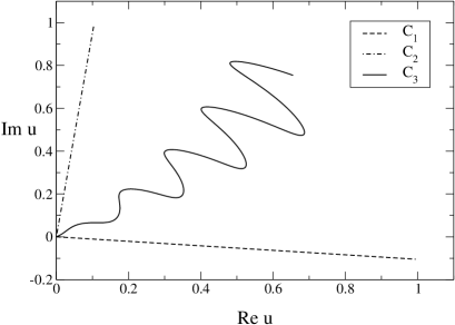
Figure 1: Three examples of integration contours in the $u$-plane.

Figure 2: Three regions ${\cal T}_{\varepsilon,k}$ in the complex $\lambda$ plane given by Eq. (14), for the three contours ${\cal C}_{k}$ shown in Fig. 1. If $\varepsilon$ is small, 0.05 say (left panel), all the three angles are large, though ${\cal T}_{\varepsilon,3}$ is smaller than the other two. For $\varepsilon=1.2$ (right panel), $\varepsilon$ is near the upper limit 1.27 imposed by condition (10) for $k=3$; as a consequence, the angle ${\cal T}_{\varepsilon,3}$ is very narrow.

Remark 9: We note that the parametrization $G(r)=r\exp{(ig(r))}$ does not include contours that cross a circle centred at $r=0$ either touching or doubly intersecting it, so that the derivative $G^{\prime}(r)$ does not exist or is not bounded. In particular, this parametrization does not include the contours

(i) that, starting from the origin and reaching a value $r_{1}$ of $r$, return back to a certain value $r_{2}<r_{1}$, closer to the origin, and

(ii) whose one or several parts coincide with a part of a circle centred at the origin.

The contours under (i) can be included by representing the integral as a sum of several integrals along individual contours that separately fulfill the conditions of Lemma 2. In particular, if the integration contour returns back to the origin, the expansion coefficients all vanish. The cases under item (ii) can be treated by choosing an alternative parametrization of the curve.

Remark 10: Extensions of the Watson lemma to the complex plane were considered briefly by H. Jeffreys in Ref. Jeff , under somewhat different conditions.

a) Identical is the condition requiring that the function $f(u)$ is holomorphic on a disc, $|u|<R$.

b) In Ref. Jeff , the integration is performed along a right angle in the complex $u$-plane, first along the real axis and then along a segment parallel to the imaginary axis, up to the upper point of the integration contour. So, it is assumed that the integral along this right angle exists, in particular, that the function $f(u)$ is defined along it. In fact, $f$ is assumed to be analytic in the region bounded by the initial contour and this right angle, except for some isolated singularities. The condition of Lemma 2 requires only that, outside the circle, $f(u)$ is defined along the curve of the original contour of integration. These weaker assumptions imply that our approach is more general.

c) Lemma 2 and its proof allow us to use the bounds (31), (33), and (35) to obtain an estimate for the difference between $\Phi^{(G)}_{0,c}(\lambda)$ and its asymptotic expansion (13) in terms of the constants introduced in the conditions (8), (9) and (11).

d) Finally, we remind the reader that the proof of Lemma 2 in subsection V.1 allowed us to obtain a remarkable correlation between the strength of the bounds on the remainder and the size of the angles where the asymptotic expansion is valid. Indeed, (31), (33), and (35) depend on the parameter $\varepsilon$, which determines the angles $\cal T_{\varepsilon}$ and $\cal Z_{\varepsilon}$, see (14) and (49) respectively. As was pointed out in Remark 8, the larger the angle of validity, the looser the bound, and vice versa.

VII Remarks on perturbative QCD

We take the Adler function Adler

$${\cal D}(s)=-s\frac{{\rm d}\Pi(s)}{{\rm d}s}-1\,,$$ (50)

to discuss applications of Lemma 2, where $\Pi(s)$ is the polarization amplitude defined from

$$i\int{\rm d}^{4}xe^{iq.x}<0|T\{V_{\mu}(x)V_{\nu}(0)^{{\dagger}}\}|0>=(q_{\mu}q_{\nu}-g_{\mu\nu}q^{2})\Pi(s).$$ (51)

Here $s=q^{2}$ and $V_{\mu}$ is the vector current for light ($u$ or $d$) quarks.

In accordance with general principles BogSh ; Adler , ${\cal D}(s)$ is real analytic in the complex $s$-plane, except for a cut along the time-like axis produced by unitarity. In perturbative QCD, any finite-order aproximant has cuts along the time-like axis, while the renormalization-group improved expansion,

$${\cal D}(s)=D_{1}\,\alpha_{s}(s)/\pi+D_{2}\,(\alpha_{s}(s)/\pi)^{2}+D_{3}\,(\alpha_{s}(s)/\pi)^{3}+\ldots\,,$$ (52)

has in addition an unphysical singularity due to the Landau pole in the running coupling $\alpha_{s}(s)$. According to present knowledge, (52) is divergent, $D_{n}$ growing as $n!$ at large $n$ Mueller1992 -BenekePR .

VII.1 Ambiguity of the perturbative QCD

To discuss the implications of Lemma 2, we can define the Borel transform $B(u)$ by Neubert1996

$$B(u)=\sum\limits_{n\geq 0}b_{n}\,u^{n},\quad\quad\quad b_{n}=\frac{D_{n+1}}{\beta_{0}^{n}\,n!}\,.$$ (53)

It is usually assumed the series (53) is convergent on a disc of nonvanishing radius (this result was rigorously proved by David et al. David for the scalar $\varphi^{4}$ theory). This is exactly what is required in Lemma 2 for the Borel transform.

If we adopt the assumption that the series (52) is asymptotic, Lemma 2 implies a large freedom in recovering the true function from its perturbative coefficients. Indeed, taking for simplicity $\alpha=\beta=1$ in (12), we infer that all the functions ${\cal D}^{G}_{0,c}(s)$ of the form

$${\cal D}^{G}_{0,c}(s)=\frac{1}{\beta_{0}}\int_{r=0}^{c}e^{-\frac{G(r)}{\beta_{0}\,a(s)}}\,B(G(r))\,{\rm d}G(r)\,,$$ (54)

where $a(s)=\alpha_{s}(s)/\pi$, admit the asymptotic expansion

$${\cal D}^{G}_{0,c}(s)\sim\sum\limits_{n=1}^{\infty}D_{n}\,(a(s))^{n},\quad\quad\quad a_{s}(s)\to 0,$$ (55)

in a certain domain of the $s$-plane, which follows from (14) and the expression of the running coupling $a(s)$ given by the renormalization group.

As mentioned above, Lemma 2 imposes weak conditions on $B(u)$ and on the integration contour. Outside the convergence disc of (53), the form of $B(u)$ (denoted $f(u)$ in section IV) is largely arbitrary, being restricted only by the rather weak conditions of Lemma 2. If the function $B(u)$ defined by (53) admits an analytic continuation outside the disc (which is not necessary for Lemma 2 to apply), the analytic continuation can be used as input in the integral representation (55). Then, if the contour passes through the analyticity domain, ${\cal B}$ say, more specific properties of ${\cal D}^{G}_{0,c}(s)$ in the coupling plane can be derived, in analogy with the case of Borel summable functions (see Sokal ).

The integral (54) reveals the large ambiguity of the resummation procedures having the same asymptotic expansion in perturbative QCD: no particular function of the form ${\cal D}^{G}_{0,c}(s)$ can be a priori preferred when looking for the true Adler function.

The proof of Lemma 2 shows that the form and length of the contour, as well as the values of $B(u)$ outside the convergence disc, do not affect the series (55), contributing only to the exponentially suppressed remainder. As seen from the r.h.s. of (25) or (46), the terms to be added to (55) are $\Phi^{G}_{r_{0},c}(\lambda)$ and $I^{k}_{r_{0},\infty}(\lambda)$, where $\lambda=1/(\beta_{0}a(s))$. The estimates in (31) and (33) imply the remainder to (55) to have the form $h\,{\rm exp}(-d/\beta_{0}a(s))\sim h\left(-\Lambda^{2}/s\right)^{d}$, where we used the running coupling to one loop. The quantities $h$ and $d>0$ depend on the integration contour and on the values of $B(u)$ outside the disc, which can be chosen rather freely. So, (54) contains arbitrary power terms, to be added to (55).

VII.2 Optimal conformal mapping and analyticity

In problems of divergence and ambiguity, the location of singularities of ${\cal D}(s)$ and $B(u)$ in the $a(s)$-plane and, respectively, in the $u$-plane, is of importance.

Some information about the singularities of ${B(u)}$ is obtained from certain classes of Feynman diagrams, which can be explicitly summed Beneke1993 -BenekePR , and from general arguments based on renormalization theory Mueller1992 ; BeBrKi . This analysis shows that $B(u)$ has branch points along the rays $u\geq 2$ and $u\leq-1$ (IR and UV renormalons respectively). Other (though nonperturbative) singularities, for $u\geq 4$, are produced by instanton-antiinstanton pairs. Due to the singularities at $u>0$, the series (52) is not Borel summable. Except the above mentioned singularities of $B(u)$ on the real axis of the $u$-plane, however, no other singularities are known; it is usually assumed that, elsewhere, $B(u)$ is holomorphic.

To treat the analyticity properties of $B(u)$, the method of optimal conformal mapping SorJa is very useful. If the analyticity domain ${\cal B}$ is larger than the disc of convergence of (53), one replaces (53) by the expansion

$$B(u)=\sum_{n\geq 0}c_{n}\,w^{n},$$ (56)

where $w=w(u)$ (with $w(0)=0$) maps ${\cal B}$ (or a part of it) onto the disc $|w|<1$, on which (56) converges. (56) has better convergence properties than (53): in SorJa , Schwarz lemma was used to prove that the larger the region mapped by $w(u)$ onto $|w|<1$, the faster the convergence rate of (56).

If $w(u)$ maps the whole ${\cal B}$ onto the disc $|w|<1$, (56) converges on the whole region ${\cal B}$ and, as shown in SorJa , its convergence rate is the fastest. Then, the region of convergence of (56) coincides with the region ${\cal B}$ of analyticity of $B(u)$.

Optimal conformal mapping allows one to express analyticity in terms of convergence. Inserting (56) into (54) we have

$${\cal D}^{G}_{0,c}(s)=\frac{1}{\beta_{0}}\int_{r=0}^{c}e^{-\frac{G(r)}{\beta_{0}\,a(s)}}\,\sum_{n\geq 0}c_{n}\,[w(G(r))]^{n}\,{\rm d}G(r)\,.$$ (57)

This expression admits the same asymptotic expansion (55). However, containing powers of the variable $w$, it implements more information about the singularities of the true Borel transform $B(u)$ than the series (53) in powers of $u$, even at finite orders. So, one expects that the finite-order approximants of (57) will provide a more accurate description of the physical function searched for CaFi ; CvLe .

VII.3 Piecewise analytic summation

The choice of the integration contour may have a fateful impact on analyticity. In HoMa ; BrMa , two different contours in the $u$-plane are chosen for the summation of some class of diagrams (the so-called renormalon chains Beneke1993 ; Broad1993 ): one contour, parallel and close to the positive semiaxis, is adopted for $a(s)>0$, another one, parallel and close to the negative semiaxis, is taken when $a(s)<0$. As was expected, and later proved in CaFi4 , analyticity is lost with this choice, the summation being only piecewise analytic in $s$. Although this summation represents only a part of the full correlator, it is preferable to approximate an analytic correlator by a function which is also analytic, since analyticity in the $s$-plane is needed for relating perturbative QCD in the Euclidean region to measurable quantities on the time-like axis.

On the other hand, as shown in CaNe ; CaFi3 , the Borel summation with the Principal Value (PV) prescription of the same class of diagrams admits an analytic continuation to the whole $s$-plane, being consistent with analyticity except for an unphysical cut along a segment of the space-like axis, related to the Landau pole. In this sense, PV is an appropriate prescription.

VIII Concluding remarks

The main result of our work is a modified form of Watson’s lemma on asymptotic series. This result, referred to as Lemma 2, holds if the function $f(u)$ (which corresponds to the Borel transform of a QCD correlator) is analytic in a disc and is defined along a contour, on which it satisfies rather weak conditions, which are specified in section IV.

Our result emphasizes the great ambiguity of the summation prescriptions that are allowed if the perturbation expansion in QCD is regarded as asymptotic. The contour of the integral representing the QCD correlator and the function $B(u)$ can be chosen very freely outside the convergence disc.

We kept our discussion on a general level, bearing in mind that little is known, in a rigorous framework, about the analytic properties of the QCD correlators in the Borel plane. If some specific properties are known or assumed, the integral representations discussed in ths paper will have additional analytic properties, known to be shared also by the physical amplitudes.

Lemma 2 proved in this paper may also be useful in other branches of physics where perturbation series are divergent.

- (1) F.J. Dyson, Phys. Rev. 85, 631 (1952)
- (2) B. Lautrup, Phys. Lett. B69, 109 (1977).
- (3) L.N. Lipatov, Sov. Phys. JETP 45, 216 (1977).
- (4) G. Parisi, Phys. Lett. B76, 65 (1978).
- (5) G. ’t Hooft, in: The Whys of Subnuclear Physics, Proceedings of the 15th International School on Subnuclear Physics, Erice, Sicily, 1977, edited by A. Zichichi (Plenum Press, New York, 1979), p. 943.
- (6) A.H. Mueller, Nucl. Phys. B250, 327 (1985).
- (7) J. Fischer, Fortsch. Phys. 42, 665 (1994); Int. J. Mod. Phys. A12, 3625 (1997).
- (8) D.I. Kazakov and D.V. Shirkov, Fortsch.Phys. 28, 465 (1980).
- (9) D.I. Kazakov and V.S. Popov, J.Exp.Theor.Phys 95, 581 (2002).
- (10) S.L. Adler, Phys. Rev. D10, 3714 (1974).
- (11) H. Jeffreys, Asymptotic Approximations (Clarendon Press, Oxford, 1962).
- (12) R.B. Dingle, Asymptotic Expansions: Their Derivation and Interpretation (Academic Press, 1972).
- (13) M.V. Fedoryuk, Asymptotics, Integrals and Series (in Russian), Moscow, Nauka, 1987, p. 58
- (14) N.N. Bogoliubov and D.V. Shirkov, Introduction to the Theory of Quantized Fields (Interscience, New York, 1959).
- (15) A.H. Mueller, in QCD - Twenty Years Later, Aachen 1992, edited by P. Zerwas and H. A. Kastrup (World Scientific, Singapore, 1992).
- (16) M. Beneke, Nucl. Phys. B405, 424 (1993).
- (17) D.J. Broadhurst, Z. Phys. C58, 339 (1993).
- (18) M. Neubert, Nucl. Phys. B463, 511 (1996).
- (19) M. Beneke, Phys. Rept. 317, 1 (1999).
- (20) F. David, J. Feldman and V. Rivasseau, Comm. Math. Phys. 116, 215 (1988).
- (21) A.D. Sokal, J. Math. Phys. 21, 261 (1980).
- (22) M. Beneke, V.M. Braun and N. Kivel, Phys. Lett. B404, 315 (1997).
- (23) J. Chýla, Czech. J. Phys. 42, 263 (1992).
- (24) S. Ciulli and J. Fischer, Nucl. Phys. 24, 465 (1961).
- (25) I. Caprini and J. Fischer, Phys. Rev. D60, 054014 (1999); Phys .Rev. D62, 054007 (2000).
- (26) D.E. Soper and L.R. Surguladze, Phys. Rev. D54, 4566 (1996).
- (27) G. Cvetic̆ and T. Lee, Phys. Rev. D64, 014030 (2001).
- (28) D.M. Howe and C.J. Maxwell, Phys. Rev. D 70, 014002 (2004)
- (29) P.M. Brooks, and C.J. Maxwell, Phys. Rev. D74, 065012 (2006).
- (30) I. Caprini and J. Fischer, Phys. Rev. D76, 018501 (2007).
- (31) I. Caprini and M. Neubert, JHEP 03, 007 (1999).
- (32) I. Caprini and J. Fischer, Phys. Rev. D71, 094017 (2005).