Non-stationary parabolic equations for the quasi-monochromatic sound propagation in media with a non-stationary background flow

Abstract

The narrow and wide-angle parabolic equations for the quasi-monochromatic sound wave packets propagating in a waveguide with a non-stationary background flow are obtained. The results of numerical simulations are presented.

1 Introduction

Parabolic equations for sound propagation in moving media were reported by many authors, but any systematic derivation of such equations on the base of some universal asymptotic method was not presented in the literature yet. In this paper we use the generalized multiple-scale method [1] to obtain some equations of this type. The material of this paper was presented at the seminar “Acoustics of inhomogeneous media X”, Novosibirsk, Russia, 1-6 June 2009.

2 Derivation of equations

We start with the equation [2]

$$D_{t}\frac{\partial}{\partial t}\left(\frac{1}{\rho c^{2}}D_{t}p\right)-\mathop{\rm div}\nolimits\frac{\partial}{\partial t}\left(\frac{1}{\rho}\mathop{\rm grad}\nolimits p\right)+2\cdot\sum_{ij}\frac{\partial\mathbf{V}_{i}}{\partial x_{j}}\frac{\partial}{\partial x_{i}}\left(\frac{1}{\rho}\frac{\partial p}{\partial x_{j}}\right)=0\,,$$ (1)

where $\mathbf{V}=(V_{1},V_{2},V_{3})=(u,w,v)$ is the velocity vector of the background flow written on the orthogonal coordinate system $(x,y,z)$ ($z$-axis is directed upward), $D_{t}=(\partial/\partial t+u\partial/\partial x+w\partial/\partial y+v\partial/\partial z)$, $p$ is the acoustic pressure.

Let $\epsilon$ be a small parameter, which is the ratio of characteristic wave length to the characteristic size of the medium inhomogeneties. Following the generalized multiple-scale metod [1] we rewrite (1) using the slow variables $T=\epsilon t$, $X=\epsilon x$, $Y=\epsilon^{1/2}y$, $Z=\epsilon^{1/2}z$ and the fast variable $\eta=(1/\epsilon)\theta(X,Y,Z,T)$. We will assume that the flow velocity is $O(\epsilon)$ and then $u=\epsilon U(X,Y,Z,T)$, $w=\epsilon^{3/2}W(X,Y,Z,T)$ and $v=\epsilon^{3/2}V(X,Y,Z,T)$, where the quantities $U$, $W$ and $V$ are$O(1)$. We introduce for convenience the quantity $n=1/c$ and postulate the expansions

$$n^{2} = n_{0}^{2}(X,Y,T)+\epsilon\nu(X,Y,Z,T)\,,$$

$$p = p_{0}(X,Y,T,Z,\eta)+\epsilon p_{1}(X,Y,T,Z,\eta)+\ldots\,,$$

The density will be assumed depending on the slow variables only, $\rho=\rho(X,Y,Z,T)$. At last, the partial derivatives are transformed by the rules

$$\frac{\partial}{\partial x}\rightarrow\epsilon\frac{\partial}{\partial X}+\theta_{X}\frac{\partial}{\partial\eta}\,,\qquad\frac{\partial}{\partial y}\rightarrow\epsilon^{1/2}\frac{\partial}{\partial Y}+\epsilon^{-1/2}\theta_{Y}\frac{\partial}{\partial\eta}\,,$$

analogously for the variables $t$ $z$. In the rewritten in such a way (1) we collect terms with like degrees of $\epsilon$. The squares of the background flow velocities will be neglected as they was neglected in the derivation of (1).

At $O(\epsilon^{-1}$ we obtain that the phase function $\theta$ does not depend on variables $Z$ $Y$, $\theta=\theta(X,T)$.

At $O(\epsilon^{0}$ we obtain the Hamilton-Jacobi equation

$$\left(\theta_{X}\right)^{2}-n_{0}^{2}\left(\theta_{T}\right)^{2}=\left(\theta_{X}+n_{0}\theta_{T}\right)\left(\theta_{X}-n_{0}\theta_{T}\right)=0\,.$$ (2)

We shall consider the waves propagating in the positive $X$-direction and adopt as the Hamilton-Jacoby equation the first factor in (2).

The equation at $O(\epsilon^{1})$ does not contain $p_{1}$ on the strength of (2). Substituting in this equation the anzats $p_{0}=A_{0}(X,Y,T,Z)\exp(\mathrm{i}\eta)$, we obtain the equation for the amplitude $A_{0}$

$$2\mathrm{i}n_{0}\omega\frac{1}{\rho}\left[A_{0,X}+n_{0}A_{0,T}\right]+\left(\frac{1}{\rho}A_{0,Y}\right)_{Y}+\left(\frac{1}{\rho}A_{0,Z}\right)_{Z}+\chi A_{0}=0\,,$$ (3)

where $\omega=-\theta_{T}$ is the local frequency of sound,

$$\chi=\left\{\left[\left(\frac{1}{\rho}n_{0}\right)_{X}+n_{0}\left(\frac{1}{\rho}n_{0}\right)_{T}\right]\omega\mathrm{i}+\frac{1}{\rho}\left(\nu-2n_{0}^{3}U\right)\omega^{2}\right\}\,.$$ (4)

Assuming that

$$\nu=-2\frac{c_{1}}{c_{0}^{3}}\,,$$

where $c_{0}=1/n_{0}$, we obtain that

$$\frac{1}{\rho}\omega^{2}\nu-2\frac{1}{\rho}\omega^{2}n_{0}^{3}U=2\frac{1}{\rho}\omega^{2}\frac{c_{1}+U}{c_{0}^{3}}\,,$$

so the potential of the parabolic equation contains the so called effective sound speed $c+U$, as was first shown in the paper [3]. We see that our equation is a generalization of the parabolic equation obtained in that work.

Note that the dependence on variable $Y$ in the obtained equation is just the same as on $Z$. Therefore in the sequel we shall not write the terms expressing the dependence on $Y$ and consider the $2D$ waveguide. As will be easily seen, all result can be directly transferred to the $3D$ case.

The analogous considerations at $O(\epsilon^{2})$ gives the equation for the amplitude $A_{1}$, $p_{1}=A_{1}(X,Z,T)\exp(\mathrm{i}\eta)$.

$$2\mathrm{i}n_{0}\omega\frac{1}{\rho}\left[A_{1X}+n_{0}A_{1T}\right]+\left(\frac{1}{\rho}A_{1Z}\right)_{Z}+\chi A_{1}+{\cal F}=0\,,$$ (5)

where

$$\begin{split}{\cal F}=&\left(\frac{1}{\rho}A_{0X}\right)_{X}-\left(\frac{1}{\rho}n_{0}^{2}A_{0T}\right)_{T}+2\mathrm{i}\frac{1}{\rho}\nu\omega A_{0T}+\mathrm{i}\left(\frac{1}{\rho}\nu\omega_{T}\right)_{T}A_{0}\\ &-\frac{\mathrm{i}}{\omega}U\left(\frac{1}{\rho}n_{0}^{2}\omega^{2}A_{0}\right)_{X}-3\mathrm{i}U\frac{1}{\rho}n_{0}^{2}\omega A_{0X}-2\mathrm{i}U_{X}\frac{1}{\rho}n_{0}^{2}\omega A_{0}\\ &+\mathrm{i}\left[\left(\frac{1}{\rho}n_{0}\right)_{X}-\frac{1}{\rho}n_{0}n_{0T}\right]Un_{0}\omega A_{0}-\mathrm{i}\frac{1}{\omega}V\left(n_{0}^{2}\omega^{2}\frac{1}{\rho}A_{0}\right)_{Z}\\ &-\mathrm{i}\frac{1}{\rho}n_{0}^{2}\omega VA_{0Z}-Un_{0}\left(\frac{1}{\rho}A_{0Z}\right)_{Z}-2U_{Z}\frac{1}{\rho}A_{0Z}\,,\end{split}$$ (6)

It can be shown [4] that the system of equations (3), (5) generalize the known wide-angle stationary parabolic equation obtained by the factorization method with the rational-linear Padé approximation of the square root operator. Moreover, even in the stationary case our equations contains the terms that the factorization method cannot produce.

3 Initial-boundary value problems for the parabolic equations

For the simulation of the sound waves in the ocean the most interesting initial-boundary value problems for the Hamilton-Jacobi equatuion (2) and the parabolic equations (3), (5) are the problems with $X$ as the evolution variable in the domain $\Omega=\{Z_{0}<Z<Z_{1}\}\times\{T_{0}<T<T_{1}\}$.

For the energy norm

$$E(X)=\int_{T_{0}}^{T_{1}}\int_{Z_{0}}^{Z_{1}}\frac{1}{\rho}|\theta_{X}A_{0}|^{2}\,dZdT\,.$$

under some simple and natural assumptions on the boundary conditions at $\partial\Omega$, the following theorem holds

Theorem 1.

The energy norm of the solution of the initial-boundary value problem for the parabolic equation (3) satisfies the inequality

$$E(X)\leq E(0)\cdot\exp\left(\int_{0}^{X}\sup_{T}\left(\frac{n_{0,s}(s,T)}{n_{0}(s,T)}\right)\,ds\right)$$ (7)

If $n_{0}$ can be represented in the form $n_{0}=\bar{n}_{0}(X)a(T)$ then the following inequality holds

$$E(X)\leq E(0)\frac{\bar{n}_{0}(X)}{\bar{n}_{0}(0)}\sup_{T}a(T)\,.$$ (8)

This theorem immediately implies the uniqueness of solutions of such initial-boundary value problems for (3), (5) in functional spaces of the type $C([0,X],L_{2}(\Omega))$.

4 Numerical simulation

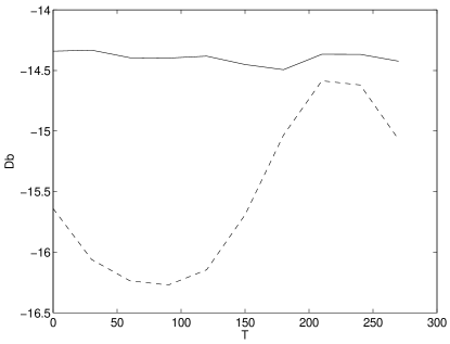
Figure 1: Temporal variations of the transmission loss at the distance 6 km (left) and 12 km (right): with the velocity terms (dashed line), without these terms (solid line). The second mode of internal waves.

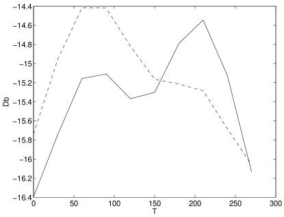
Figure 2: Temporal variations of the transmission loss at the distance 6 km (left) and 12 km (right): with the velocity terms (dashed line), without these terms (solid line). The third mode of internal waves.

In the parabolic equations (3), (5) the influence of the background flow is taken into account not only through the terms which explicitly contain the corresponding velocities, but also through the deformation of the sound speed and density profiles. As the geometric small parameter $\epsilon$ in typical cases is much larger than the Mach number for the ocean medium, the question about essentiality of introducing the background flow velocities in the narrow-angle parabolic equation (3) is naturally risen.

For an answer to this question the simulation of the harmonic sound wave propagation through the harmonic internal wave of a given mode was conducted, with the following parameters: the undisturbed waveguide of constant depth (100 m) was given by the parabolic sound speed profile with the minimum (1460 m/s) at the center of the waveguide and maximum (1500 m/s) at the top and bottom boundaries, the sound frequency was taken to be equal 100 Hz and the boundary conditions for the sound field was taken to be soft at the top boundary and hard at the bottom boundary. The point sound source was situated at the center of the waveguide. The density stratification was given by the constant Brent-Väsälä frequency ($1/127~{}\text{s}^{-1}$), for the simulation were used the five minutes period internal waves of the second mode (wavelength=214 m) and the third mode (wavelength=142 m).

The results are presented in fig. 1,2 in the form of the temporal variations of the transmission loss at the distances of 6 km and 12 km from the source. We can conclude that the explicit introduction of the background flow velocities to the narrow-angle parabolic equation is essential.

5 Conclusion

In this paper the system of parabolic-like equations (3), (5), which can be used for numerical modelling of sound propagation in waveguides with non-stationary background flow, is obtained. Some properties of these equations are established. We hope that this information will be useful for the computational acoustics community. Complete derivations, proofs and more extensive numerical modelling will be presented in the forthcoming paper.

References

• [1] Nayfeh, A. H. Perturbation methods. John Wiley & Sons, N.-Y., 1973.
• [2] Ostashev, V. E. Sound propagation in moving media. Nauka, Moscow, 1992. (in Russian)
• [3] Nghuem-Ohu, L., Tappert, F. Parabolic equation modeling of the effects of ocean currents on sound tranmission and reciprocity in the time domain. J. Acoust. Soc. Amer., v. 78, 1985, no. 2, pp. 642-648.
• [4] Trofimov, M. Yu. Time-dependent parabolic equations for two-dimensional waveguides. Technical Physics Letters v. 26, 2000 no. 9, pp. 797-798.