Many-body position operator in lattice fermionic systems with periodic boundary conditions

Abstract

A total position operator $X$ in the position representation is derived for lattice fermionic systems with periodic boundary conditions. The operator is shown to be Hermitian, the generator of translations in momentum space, and its time derivative is shown to correspond to the total current operator in a periodic system. The operator is such that its moments can be calculated up to any order. To demonstrate its utility finite size scaling is applied to the Brinkman-Rice transition as well as metallic and insulating Gutzwiller wavefunctions.

Short title: Periodic lattice position operator

The position operator and its moments give important information about localization in quantum systems. As was shown by Kohn [1] metals and insulators are distinguished by the extent of their localization. Many real systems are periodic, and in many model systems periodic boundary conditions are imposed. In such cases the Hilbert space which that forms the domain of operators is restricted hence the position operator is ill-defined [2]. The single particle position operator in the crystal momentum representation was derived by Blount [2] and discussed extensively in the context of band-theory. In the crystal momentum representation this operator can be generalized to the many-body case [3]. To calculate the total position in the position representation Resta [4, 5] suggests to average the quantity $e^{i\frac{2\pi x}{L}}$. The expectation value of the total position operator is then defined as

$$\langle x\rangle=\frac{L}{2\pi}\mbox{Im}\hskip 3.61371pt\mbox{ln}\langle\Psi|e^{i\frac{2\pi x}{L}}|\Psi\rangle.$$ (1)

Via first order perturbation theory, Resta also shows [4] that the time derivative of the polarization operator based on the above definition gives the total current in the limit $L\rightarrow\infty$. This idea has been applied to lattice fermionic systems at half-filling [5], and extended to systems at arbitrary fillings [6]. A related formalism due to Souza et al. [7] based on the cumulant generating function (of which Eq. (1) is a special case) establishes relations between localization and polarization.

It is important to note that the position operator in this method is calculated indirectly, by first evaluating the expectation value of $e^{i\frac{2\pi x}{L}}$. Eq. (1) is valid as can be shown [5] but the calculation of higher moments is not straight forward, the spread functional suggested by Resta and Sorella [5] (based on eq. (1)) is valid in the thermodynamic limit.

Here it is shown that a total position operator for a lattice fermionic system with periodic boundary conditions can be defined as the generator of total momentum shifts. It is also demonstrated that the time derivative of the total position operator gives the current for a system with any number of sites (finite $L$). The total position operator derived below is such that expectation values of arbitrary powers are readily evaluated, hence an accurate assessment and finite size scaling of localization is enabled (up to any desired order). The utility of the operator is then demonstrated via variational calculations on the Hubbard model [8, 9, 10] based on the Gutzwiller wavefunction [10, 11].

The derivation of the total position operator is closely related to that of the total momentum operator in Ref. [12]. The class of models for which the formalism presented below are those used in strongly correlated systems consisting of site to site hopping terms and some interaction terms. An example of a lattice model is the Hubbard Hamiltonian,

$$H=-t\sum_{\langle i,j\rangle\sigma}(c_{i\sigma}^{\dagger}c_{j\sigma}+H.c.)+U\sum_{i\sigma}n_{i\uparrow}n_{i\downarrow},$$ (2)

consisting of $L$ sites. In the following, the total position operator will be derived for the one-dimensional Hubbard model. Generalizations to higher dimensions and other lattice models will be discussed below.

The real-space (Wannier state) and reciprocal-space (Bloch state) creation operators are related in the usual way,

$$\tilde{c}_{k}=\frac{1}{\sqrt{L}}\sum_{j=1}^{L}e^{i\frac{2\pi kx_{j}}{L}}c_{j},$$ (3)

where $x_{j}$ is the position of site $j$. In order to define a total position operator we first define a momentum permutation operator as

$$P_{kl}=1-(\tilde{c}^{\dagger}_{k}-\tilde{c}^{\dagger}_{l})(\tilde{c}_{k}-\tilde{c}_{l}),$$ (4)

where $\tilde{c}^{\dagger}_{k}$ creates a particle in the Bloch state $k$. A momentum space shift operator can be defined as

$${\mathfrak{U}}_{n}=P_{n-1n}....P_{12},$$ (5)

with the property that

$${\mathfrak{U}}_{L}\tilde{c}_{k}=\left\{\begin{array}[]{rl}\tilde{c}_{k-1}{\mathfrak{U}}_{L},&k=2,...,L\\ \tilde{c}_{L}{\mathfrak{U}}_{L},&k=1.\end{array}\right.$$ (6)

For systems with spin-$\frac{1}{2}$ particles we can define the compound momentum space shift operator as

$${\mathfrak{U}}={\mathfrak{U}}_{L\uparrow}{\mathfrak{U}}_{L\downarrow},$$ (7)

with the property

$${\mathfrak{U}}c_{j,\sigma}=e^{i\frac{2\pi x_{j}}{L}}c_{j,\sigma}{\mathfrak{U}},$$ (8)

where $c_{j,\sigma}$ is an annihilation operator for particles at site $x_{j}$ with spin $\sigma$.

We define the total position operator $X$ through three conditions. First we require it to be the generator of total momentum shifts, i.e.

$${\mathfrak{U}}=e^{i\frac{2\pi X}{L}}.$$ (9)

We also require $X$ to be Hermitian,

$$X=X^{\dagger}.$$ (10)

and that the time derivative of $X$ give the total current,

$$e\dot{X}=ie[H,X]=J,$$ (11)

which for the Hubbard model is defined as

$$J=-iet\sum_{\langle i,j\rangle\sigma}(c_{i\sigma}^{\dagger}c_{j\sigma}-c_{j\sigma}^{\dagger}c_{i\sigma}).$$ (12)

In order to derive the explicit form of $X$ we first define

$$g(\alpha)=\sum_{x=0}^{L-1}ie^{-i\frac{2\pi x\alpha}{L}},$$ (13)

which can be evaluated via the geometric sum formula to give

$$g(\alpha)=i\frac{1-e^{-i2\pi\alpha}}{1-e^{-i\frac{2\pi\alpha}{L}}}.$$ (14)

We can take the derivative of $g(\alpha)$ at some integer value $m$ for $\alpha$,

$$g^{\prime}(m)=\frac{2\pi}{L}\sum_{x=0}^{L-1}xe^{-i\frac{2\pi xm}{L}}.$$ (15)

Inverting the Fourier series, we can obtain an expression for the position $x$ valid for $x=0,...,L-1$,

$$x=\frac{1}{2\pi}\sum_{k=1}^{L}g^{\prime}(m)e^{i\frac{2\pi xm}{L}}.$$ (16)

For $m\neq L$,

$$g^{\prime}(m)=2\pi/(e^{-i\frac{2\pi m}{L}}-1),$$ (17)

and $g^{\prime}(L)$ can be evaluated from Eq. (15) using the arithmetic sum formula giving $g^{\prime}(L)=\pi(L-1)$. Thus, an overall expression for $x$ reads as

$$x=\sum_{m=1}^{L-1}\left(\frac{1}{2}+\frac{e^{-i\frac{2\pi xm}{L}}}{e^{-i\frac{2\pi m}{L}}-1}\right).$$ (18)

The right hand side of Eq. (18) is the sawtooth function $f(x)=x\mbox{mod}L$. We propose to take the sawtooth function as the definition of our position operator. Based on Eq. (9) we write the total position operator $X$ for a many-particle system as a power series in the momentum shift operator as

$$X=\sum_{m=1}^{L-1}\left(\frac{1}{2}+\frac{{\mathfrak{U}}^{m}}{e^{-i\frac{2\pi m}{L}}-1}\right).$$ (19)

It is to be emphasized that $X$ is a genuine many-body operator (as is that of Resta [4]).

Having defined our total position operator, we can now test whether it satisfies the requirements (Eqs. (9), (10), and (11)). Letting $X$ operate on an arbitrary Wannier state ($|{\bf x},{\bf\sigma}\rangle=c_{1,\sigma_{1}}^{\dagger}...c_{N,\sigma_{N}}^{\dagger}|0\rangle$) for a system gives the result

$$X|{\bf x},{\bf\sigma}\rangle = \sum_{m=1}^{L-1}\left(\frac{1}{2}+\frac{e^{i\frac{2\pi m(x_{1}+...+x_{N})}{L}}}{e^{-i\frac{2\pi m}{L}}-1}\right)|{\bf x},{\bf\sigma}\rangle$$ (20)

$$= ((x_{1}+...+x_{L})\mbox{mod}L)|{\bf x},{\bf\sigma}\rangle$$ (21)

where we have used Eqs. (8) and (18). Since

$${\mathfrak{U}}|{\bf x},{\bf\sigma}\rangle=e^{i\frac{2\pi(x_{1}+...+x_{N})}{L}}|{\bf x},{\bf\sigma}\rangle,$$ (22)

Eq. (9) follows. Hermiticity of $X$ follows from the unitarity of ${\mathfrak{U}}$ and from the fact that ${\mathfrak{U}}^{L}=1$.

To demonstrate that the operator $X$ satisfies the condition in Eq. (11), we first note that ${\mathfrak{U}}$ commutes with the interaction part of the Hamiltonian. This can be shown using Eq. (8). Thus our task consists of evaluating the commutator $[T,X]$, $T$ denoting the kinetic part of the Hubbard Hamiltonian. We first define an operator

$$Y=\sum_{m=1}^{L}\frac{{\mathfrak{U}}^{m}}{e^{-i\frac{2\pi m}{L}}-1}.$$ (23)

The last term in the sum is divergent. However, below we show that this divergence disappears for the commutator $[T,Y]$.

We first evaluate the commutator

$$[T,Y]=\sum_{m=1}^{L}\frac{[T,{\mathfrak{U}}^{m}]}{e^{-i\frac{2\pi m}{L}}-1}.$$ (24)

We split the kinetic energy in two parts as

$$A = -t\sum_{\langle i,j\rangle\sigma}c_{i\sigma}^{\dagger}c_{j\sigma}$$ (25)

$$A^{\dagger} = -t\sum_{\langle i,j\rangle\sigma}c_{j\sigma}^{\dagger}c_{i\sigma},$$ (26)

thus we can rewrite Eq. (24) as

$$[T,Y]=\sum_{m=1}^{L}\frac{[A,{\mathfrak{U}}^{m}]+[A^{\dagger},{\mathfrak{U}}^{m}]}{e^{-i\frac{2\pi m}{L}}-1}.$$ (27)

Each commutator in Eq. (27) can be evaluated using Eq. (8). We obtain

$$[A,{\mathfrak{U}}^{m}] = (e^{-i\frac{2\pi m}{L}}-1){\mathfrak{U}}^{m}A$$ (28)

$$\mbox{[}A^{\dagger},{\mathfrak{U}}^{m}\mbox{]} = (1-e^{-i\frac{2\pi m}{L}})A^{\dagger}{\mathfrak{U}}^{m},$$ (29)

giving a new expression for the commutator

$$[T,Y]=\sum_{m=1}^{L}{\mathfrak{U}}^{m}A-A^{\dagger}{\mathfrak{U}}^{m}.$$ (30)

We now substitute the condition in Eq. (9) and we obtain

$$[T,Y]=\sum_{m=1}^{L}e^{i\frac{2\pi Xm}{L}}A-A^{\dagger}e^{i\frac{2\pi Xm}{L}}.$$ (31)

It is easily seen that this commutator is zero, since $X$ operating on a Wannier state gives an integer and

$$\sum_{m=1}^{L}e^{i\frac{2\pi Xm}{L}}=0.$$ (32)

On the other hand, using the same reasoning we used to arrive at Eq. (30) it can be shown that

$$[T,X]=\sum_{m=1}^{L-1}{\mathfrak{U}}^{m}A-A^{\dagger}{\mathfrak{U}}^{m},$$ (33)

hence, from Eq. (30) we see that

$$[T,X]=A^{\dagger}-A,$$ (34)

since ${\mathfrak{U}}^{L}=1$. From Eq. (34) the expression for the current (Eq. (12)) follows straightforward.

The total position operator $X$ derived above can be generalized to many dimensions as follows. In higher dimensions the operator becomes a vector operator. The generalization of the above derivation has to be based on a generalized total momentum shift operator consisting of the product of all one-dimensional momentum shift operators in a particular direction. For example, for a three dimensional system with dimensions $x,y,z$ a total momentum shift operator for the $x$ direction (spinless case) would consist of the product of all one dimensional momentum shift operators

$${\mathfrak{W}}_{L,x}=\prod_{y,z}{\mathfrak{U}}_{L,x}^{(y,z)},$$ (35)

where ${\mathfrak{U}}_{L,x}^{(y,z)}$ denotes the total momentum shift operator in the $x$-direction for a given set of coordinates $y,z$ (Eq. (5)). Such an operator satisfies the commutation relation

$${\mathfrak{W}}_{L,x}\tilde{c}_{k_{x},k_{y},k_{z}}=\left\{\begin{array}[]{rl}\tilde{c}_{k_{x}-1,k_{y},k_{z}}{\mathfrak{W}}_{L,x},&k_{x}=2,...,L;k_{y},k_{z}=1,...,L\\ \tilde{c}_{L,k_{y},k_{z}}{\mathfrak{W}}_{L,x},&k_{x}=1;k_{y},k_{z}=1,...,L.\end{array}\right.$$ (36)

Subsequent construction of a total position operator for a three dimensional systems follows the same steps as the one-dimensional case. The total momentum shift operator for a spin-$\frac{1}{2}$ system can be written as

$${\mathfrak{W}}_{i}={\mathfrak{W}}_{L,i,\uparrow}{\mathfrak{W}}_{L,i,\downarrow},$$ (37)

where ${\mathfrak{W}}_{i}$ is a vector operator, and $i=x,y,z$. A particular component of the total position operator can then be written as

$$R_{i}=\sum_{m=1}^{L-1}\left(\frac{1}{2}+\frac{{\mathfrak{W}}_{i}^{m}}{e^{-i\frac{2\pi m}{L}}-1}\right).$$ (38)

The commutator of operator $R_{i}$ will give the current in the $i$ direction. This is a consequence of the fact that the operator ${\mathfrak{W}}_{i}$ commutes with the hoppings in directions other than $i$ included in the Hubbard Hamiltonian.

Extensions of the Hubbard model can also be handled. More complex interaction types (nearest neighbor, etc.) follow the same derivation as above, as the expression for the current does not change in this case. For more complex hoppings the expression for the current is modified to include the new hoppings, but the derivation presented above is still valid.

For impurity models [13, 14] the strategy of derivation of a total position operator is modified slightly. For example, the one-dimensional periodic Anderson model, in which each site contains a set of localized $f$-orbitals, can be written as

$$H=-t\sum_{\langle i,j\rangle\sigma}(c_{i\sigma}^{\dagger}c_{j\sigma}+H.c.)+E_{f}\sum_{i,l,\sigma}n_{f}(i,l,\sigma)+\frac{1}{2}\sum_{i}\sum_{l,\sigma\neq l^{\prime},\sigma^{\prime}}U(l,l^{\prime})n_{f}(i,l,\sigma)n_{f}(i,l^{\prime},\sigma^{\prime})+H^{\prime},$$ (39)

with

$$H^{\prime}=\sum_{i,l,\sigma}\{V_{l}f^{\dagger}_{i,l,\sigma}c_{i,\sigma}+H.c.\}.$$ (40)

In Eqs. (39) and (40) $n_{f}(i,l,\sigma)$($f^{\dagger}_{i,l,\sigma}$) denotes the density(creation operator) of $f$-orbital with label $l$ at site $i$ and with spin $\sigma$. Each lattice site contains a set of $f$ orbitals, but there are no inter-site hoppings between the localized $f$-orbitals on different sites. As a consequence the current operator is the same as that of the Hubbard model, inspite of the fact that the charge density includes the $f$-orbital terms [15]. One could construct a total position operator which does not include impurity orbitals, and has the same form as $X$ derived above (only electrons in the conduction band enter the definition). As conduction takes place only on the standard lattice sites, not the ones associated with the $f$-orbitals, such an approach may in some cases be sufficient to characterize localization phenomena associated with metal-insulator transitions. However it is also possible to construct a total position operator valid for a system with the periodic Anderson Hamiltonian.

To do this one has to consider the $f$-orbitals as separate lattices, and construct a total momentum shift operator for each set of $f$-orbitals localized on different lattice sites. One can construct an operator

$${\mathfrak{V}}_{L}^{(l)}=Q_{L-1L}^{(l)}....Q_{12}^{(l)},$$ (41)

where

$$Q_{jk}^{(l)}=1-(\tilde{f}^{\dagger}_{j,l}-\tilde{f}^{\dagger}_{k,l})(\tilde{f}_{j,l}-\tilde{f}_{k,l}).$$ (42)

$\tilde{f}_{j,l}$ denotes the Fourier transform of the annihilation operators of a particular $f$-orbital,

$$\tilde{f}_{k,l}=\frac{1}{\sqrt{L}}\sum_{j=1}^{L}e^{i\frac{2\pi kx_{j}}{L}}f_{j,l}.$$ (43)

The operator in Eq. (41) satisfies the property

$${\mathfrak{V}}_{L}^{(l)}\tilde{f}_{k}=\left\{\begin{array}[]{rl}\tilde{f}_{k-1,l}{\mathfrak{V}}_{L}^{(l)},&k=2,...,L\\ \tilde{f}_{L,l}{\mathfrak{V}}_{L}^{(l)},&k=1.\end{array}\right.$$ (44)

Thus a total momentum shift operator can be constructed as

$${\mathfrak{Z}}={\mathfrak{U}}\prod_{l}{\mathfrak{V}}^{(l)},$$ (45)

where

$${\mathfrak{V}}^{(l)}={\mathfrak{V}}_{L,\uparrow}^{(l)}{\mathfrak{V}}_{L,\downarrow}^{(l)}.$$ (46)

The total momentum shift operator $\mathfrak{Z}$ can be used to construct a total position operator

$$X_{PAM}=\sum_{m=1}^{L-1}\left(\frac{1}{2}+\frac{{\mathfrak{Z}}^{m}}{e^{-i\frac{2\pi m}{L}}-1}\right).$$ (47)

The operator $X_{PAM}$ includes the positions of electrons in impurity orbitals as well as those in the conduction band. To prove that it satisfies the three required conditions proceeds as before. Proving that the time-derivative of the position operator is equal to the current is simplified by the fact that the operators $\mathfrak{V}^{m}$ commute with the periodic Anderson Hamiltonian. This is another consequence of the fact that there are no hoppings between $f$-orbitals positioned on different sites. Hence all that needs to be proven is that the commutator corresponding to $\mathfrak{U}$ gives the current operator corresponding to that of the Hubbard model [15]. This was already shown above.

The operator $X$ is well defined in the occupation number representation and it and its moments can thus be calculated in practical situations. Here we demonstrate the utility of the operator $X$ by calculating the moments and performing finite size scaling for the Gutzwiller approximate solution of the Hubbard model at half-filling. The Gutzwiller wavefunction (GWF) has the form

$$|\Psi\rangle=\exp\left(-\gamma\sum_{i}n_{i\uparrow}n_{i\downarrow}\right)|\Psi_{0}\rangle.$$ (48)

where $|\Psi_{0}\rangle$ is a noninteracting wavefunction, and $\gamma$ is a variational parameter which projects out double occupations. Most often $|\Psi_{0}\rangle$ is the Fermi sea. In this case the exact solution in one [16, 17] and infinite dimensions [18, 19] are available. At half-filling the former is metallic for finite $U$, in contradiction with the exact solution [20]. An approximate solution to the GWF due to Gutzwiller (GA) results in the Brinkman-Rice metal insulator transition [11, 21, 22]. In finite dimensions the GA is only approximate, however in infinite dimensions it correponds to the exact solution [18, 19]. In a one-dimensional system the Brinkman-Rice transition is known to occur at $U_{c}\approx 10$. If $|\Psi_{0}\rangle$ is a non-interacting antiferromagnetic wavefunction the Gutzwiller wavefunction can be made insulating [23]. In the following, to assess the localization accompanying the metal-insulator transition we calculate the quantity

$$\chi_{4}=\frac{\sqrt{\langle X^{4}\rangle-\langle X^{2}\rangle\langle X^{2}\rangle}}{L^{2}},$$ (49)

via quantum Monte Carlo methods [24, 25].

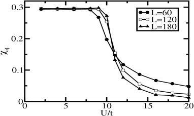
FIG. 1.: $\chi_{4}$ (defined in Eq. (49)) for the Hubbard model using the Gutzwiller wavefunction evaluated in the Gutzwiller approximation scheme. The Brinkman-Rice transition is known to occur at $U_{c}\approx 10$.

In Fig. 1 $\chi_{4}$ as a function of the Hubbard interaction strength for three different system sizes is presented. A transition at $U_{c}\approx 10$ is clearly visible from the simultaneous drop of all three curves. For large $U$ ($U\geq 11$) the largest(smallest) system shows the smallest(largest) value of the fourth moment, which is the tendency one expects for the insulating state. (The same behaviour was found for the square-root of the second order deviation.) These results coincide with what is known about the Brinkman-Rice transition being a localization transition [22].

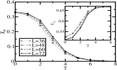
FIG. 2.: Size dependence of $\chi_{4}$ for a metallic Gutzwiller wavefunction. The inset shows the size dependence of the fourth order Binder cumulant.

In Figs. 2 and 3 a metallic and an insulating wavefunction are compared. For the former the noninteracting wavefunctions (ground state of the $U=0$ system) was used in place of $|\Psi_{0}\rangle$ in Eq. (48). For the insulating wavefunction an antiferromagnetic solution was used with a magnetization of $m=0.33333$. The size dependence of the quantity $\chi_{4}$ is clearly sensitive to whether the system is metallic or insulating: as the variational parameter $\gamma$ is increased $\chi_{4}$ decreases in both cases, but the size dependence of $\chi_{4}$ is opposite between the two cases. The metallic state (Fig. 2) shows an increase in delocalization with system size, whereas in the insulating state (Fig. 3) the larger system is more localized. The insets in Figs. 2 and 3 show the value of the fourth order Binder cumulant [26, 27, 28] defined as

$$U_{4}=1-\frac{\langle X^{4}\rangle}{3\langle X^{2}\rangle\langle X^{2}\rangle},$$ (50)

a quantity used in the finite size scaling [29] of phase transitions. $U_{4}$ approaches a value of two-thirds in the case of perfect localization. Again, total order (localization) is approached by both the metallic and insulating wavefunctions, but the size dependence is the opposite between the two cases, with the larger system closer to the limiting value of two-thirds for the insulating wavefunction (hence more localized).

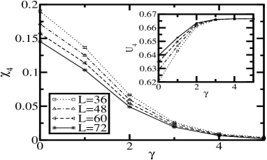
FIG. 3.: Size dependence of $\chi_{4}$ for an insulating Gutzwiller wavefunction. The inset shows the size dependence of the fourth order Binder cumulant.

In this paper a total position operator was derived for lattice models. The operator satisfies three crucial criteria: it is the generator of total momentum shifts, it is Hermitian, and its time derivative corresponds to the total current operator. The form of the operator is such that the average total position and its moments can be readily calculated. Hence Binder cumulants used in finite size scaling can also be evaluated. The sensitivity of such moments and cumulants was also demonstrated by investigating their size dependence in the Brinkman-Rice transition, and metallic and insulating Gutzwiller wavefunctions.

Part of this work was performed at the Institut für Theoretische Physik at TU-Graz under FWF (Förderung der wissenschaftlichen Forschung) grant number P21240-N16. Part of this work was performed under the HPC-EUROPA2 project (project number 228398). Helpful discussions with H. G. Evertz are gratefully acknowledged.

REFERENCES

- [1] W. Kohn, Phys. Rev., 133 A171 (1964).
- [2] E. I. Blount, Solid State Physics: Advances in Research and Applications, Eds. F. Seitz and D. Turnbull, 13 305 (1962).
- [3] N. D. M. Hine and W. M. C. Foulkes, J. Phys.: Condens. matter, 19 506212 (2007).
- [4] R. Resta, Phys. Rev. Lett., 80 1800 (1998).
- [5] R. Resta and S. Sorella, Phys. Rev. Lett., 82 370 (1999).
- [6] A. A. Aligia and G. Ortiz, Phys. Rev. Lett., 82 2560 (1999).
- [7] I. Souza, T. Wilkens, and R. M. Martin, Phys. Rev. B, 62 1666 (2000).
- [8] J. Hubbard, Proc. Roy. Soc., A276 238 (1963).
- [9] J. Kanamori, Prog. Theoret. Phys., 30 275 (1963).
- [10] M. C. Gutzwiller, Phys. Rev. Lett., 20 1445 (1963).
- [11] M. C. Gutzwiller, Phys. Rev., 137 A1726 (1965).
- [12] F. H. L. Essler, H. Frahm, F. Göhmann, A. Klümper, and V. E. Korepin, The One-Dimensional Hubbard Model, Cambridge University Press, (2005).
- [13] G. D. Mahan, Many-Particle Physics, 3rd Ed., Kluwer Academic (2000).
- [14] M. Imada, A Fujimori, and Y. Tokura, Rev. Mod. Phys., 70 1039 (1998).
- [15] D. Baeriswyl, C. Gros, and T. M. Rice, Phys. Rev. B, 35 8391 (1987).
- [16] W. Metzner and D. Vollhardt, Phys. Rev. Lett., 59 121 (1987).
- [17] W. Metzner and D. Vollhardt, Phys. Rev. B, 37 7382 (1988).
- [18] W. Metzner and D. Vollhardt, Phys. Rev. Lett., 62 324 (1989).
- [19] W. Metzner and D. Vollhardt, Helv. Phys. Acta, 63 364 (1990).
- [20] E. H. Lieb and F. Y. Wu, Phys. Rev. Lett., 20 1445 (1968).
- [21] W. F. Brinkman and T. M. Rice, Phys. Rev. B, 2 4302 (1970).
- [22] D. Vollhardt, Rev. Mod. Phys., 56 99 (1984).
- [23] W. Metzner, Z. Phys. B, 77 253 (1989).
- [24] H. Yokoyama and H. Shiba, J. Phys. Soc. Japan, 56 1490 (1986).
- [25] B. Hetényi, H. G. Evertz, and W. von der Linden, Phys. Rev. B 045107 (2009).
- [26] K. Binder, Phys. Rev. Lett., 47 693 (1981).
- [27] K. Binder, Ferroelectrics, 73 43 (1987).
- [28] K. Binder, Annu. Rev. Phys. Chem., 43 33 (1992).
- [29] M. E. Fisher and M. N. Barber, Phys. Rev. Lett., 28 1516 (1972).