Coarse-grained simulations of flow-induced nucleation in semi-crystalline polymers

Abstract

We perform kinetic Monte Carlo simulations of flow-induced nucleation in polymer melts with an algorithm that is tractable even at low undercooling. The configuration of the non-crystallized chains under flow is computed with a recent non-linear tube model. Our simulations predict both enhanced nucleation and the growth of shish-like elongated nuclei for sufficiently fast flows. The simulations predict several experimental phenomena and theoretically justify a previously empirical result for the flow-enhanced nucleation rate. The simulations are highly pertinent to both the fundamental understanding and process modeling of flow-induced crystallization in polymer melts.

I Introduction

The nucleation of microscopic crystallites in polymer liquids is profoundly influenced by flow Keller and Kolnaar (1997); Binsbergen (1966). This flow-induced crystallization (FIC), is a fascinating example of an externally driven, non-equilibrium phase transition, controlled by kinetics. Furthermore, FIC is ubiquitous in industrial processing of semi-crystalline polymers, the largest group of commercially useful polymers. A fundamental understanding of FIC promises extensive control of polymer solid state properties, as virtually every property of practical interest is determined by the crystal morphology. Flow can drastically enhance nucleation and trigger the formation of highly aligned, elongated crystals, known as shish kebabs Keller and Kolnaar (1997). Recent experiments on entangled polymers, have studied, in detail, shish kebab formation Kimata et al. (2007); Hsiao et al. (2005); Balzano et al. (2008) and the role of blend concentration Seki et al. (2002), molecular architecture Heeley et al. (2006) and molecular relaxation time Mykhaylyk et al. (2008). Often the most pronounced flow-induced effects occur near the melting point, where quiescent crystallization is immeasurably slow Binsbergen (1966); Mykhaylyk et al. (2008).

The widely postulated mechanism for FIC states that flow forces the polymer chains into elongated configurations, which lowers the entropic penalty for crystallization Keller and Kolnaar (1997). However, this hypothesis has yet to be developed into a quantitative molecular model. FIC is extremely sensitive to the flow-induced configurations of the non-crystalline chains, so an accurate molecular flow model is an essential prerequisite. Unfortunately, most polymer flow models predict only the macroscopic stress tensor and not the full molecular configuration. Alternatively, detailed simulations of polymer crystallization have provided much useful information on the growth process Waheed et al. (2005); Hu et al. (2002); Zhang and Muthukumar (2007), yet simulating primary nucleation has proven difficult, especially at low undercooling, because of the extremely long nucleation times. At a much higher level of coarse-graining, models based on differential equations either assume an empirical dependence of the nucleation rate on the flow conditions Eder and Janeschitz-Kriegl (1997), the stress tensor Zuidema et al. (2001), or the chain stretch Steenbakkers et al. (2008); or assert that free energy changes under flow can be directly subtracted from the nucleation barrier Coppola et al. (2001); Kulkarni and Beris (1999). In either case the postulated FIC mechanism remains untested. An intermediate level of coarse-graining is required to surmount these difficulties.

This letter presents coarse-grained kinetic Monte Carlo (MC) Gillespie (1977) simulations of anisotropic nucleation in flowing polymers. We compute chain configurations using a recent molecular flow model Graham et al. (2003) that reliably predicts both neutron scattering Bent et al. (2003); Blanchard et al. (2005) and bulk stresses. Our simulations predict both enhanced nucleation and elongated shish nuclei. Kinetic MC has previously been used to model quiescent crystal growth in dilute polymers Doye and Frenkel (1998). However, it is particularly suited to nucleation and our algorithm is tractable even at low undercooling, providing an efficient and highly flexible framework to simulate general anisotropic nucleation under external fields.

II Model

We compute the transient chain configuration of the uncrystallized chains under flow using the GLaMM model Graham et al. (2003), with finite chain extensibility included using Cohen’s approximation Cohen (1991). The chains are divided into $Z$ sub-chains, each corresponding to an entanglement segment of $N_{e}$ Kuhn steps of length $b$. We take $N_{e}=100$ throughout this Letter. One deterministic run of the model provides the end-to-end vector $\mathbf{f}_{i}(t)=\left<\mathbf{r}_{i}\mathbf{r}_{i}\right>$, where the ensemble average is for sub-chains of type $i$. The data for an entire transient flow are used later in the nucleation simulations. All flow timescales are in units of the subchain Rouse time $\tau_{e}$ and $\mathbf{r}$ is normalized by $\sqrt{N_{e}}b$.

Deformation of the amorphous chains has two effects on the nucleation kinetics: stretching reduces the entropic penalty for crystallization; and monomer alignment modifies the probability of compatible alignment with the nucleus. The change in elastic free energy $\Delta F^{el}$ for chains with ensemble average constraints $\mathbf{f}=\left<\mathbf{r}\mathbf{r}\right>$, but locally at equilibrium, can be calculated by statistical mechanics Olmsted and Milner (1994). Although an analytic calculation is not possible for finitely extensible chains, steep free energy gradients in highly stretched chains suppress fluctuations. Thus our numerical calculations for uniaxial deformations show that $\Delta F^{el}(\left<\mathbf{r}\mathbf{r}\right>)$ can be accurately approximated by an expression that interpolates between Gaussian elasticity Olmsted and Milner (1994) for small $\mathrm{Tr}\,{\mathbf{f}}$ and Cohen’s Cohen (1991) approximation with $\mathbf{r}^{2}=\mathrm{Tr}\,{\mathbf{f}}$ at high stretching,

$$\Delta F^{el}=\frac{1}{2}\mathrm{Tr}\,\mathbf{f}-\frac{1}{2}\mathrm{Tr}\,\ln\mathbf{f}-N_{e}\ln\left(1-\frac{\mathrm{Tr}\,\mathbf{f}}{N_{e}}\right).$$ (1)

Similarly, numerical calculation of the monomer orientation distribution $w(\theta)$ for chains with a constraint $\mathbf{f}$ are well approximated by using $\mathbf{r}^{2}=\mathrm{Tr}\,{\mathbf{f}}$ in the expression for $w(\theta)$ derived from a direct constraint on $\mathbf{r}$ Jarecki (2007).

$$\begin{array}[]{l}w(\theta)=\frac{\mathcal{L}^{-1}[\sqrt{\mathrm{Tr}\,{\mathbf{f}}}/N_{e}]}{4\pi\sinh(\mathcal{L}^{-1}[\sqrt{\mathrm{Tr}\,{\mathbf{f}}}/N_{e}])}\cosh\left(\mathcal{L}^{-1}\left[\frac{\sqrt{\mathrm{Tr}\,{\mathbf{f}}}}{N_{e}}\right]\cos\theta\right),\end{array}$$

where $\mathcal{L}^{-1}$ is the inverse Langevin function and $\theta$ is the angle between the monomer and the principle axis of $\mathbf{f}$. Each subchain has an individual $\mathbf{f}_{i}$ so is treated as a separate species with concentration $\phi_{i}=1/Z$.

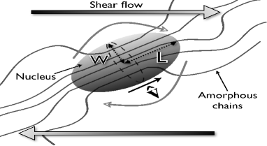
Figure 1: A sheared nucleus with protruding amorphous chains.

Our coarse-grained simulations use the minimal nucleus description required for anisotropic nucleation. The nucleus comprises $N_{T}$ crystallized “monomers” or Kuhn steps, arranged in stems, with each stem formed from a single chain (see fig 1). The total number of stems $N_{s}$ and the number of monomers in each stem is simulated. The arrangement of the monomers within the crystal is not resolved. The nucleus is assumed to be spheroidal with the polar radius $L$ parallel to the stems. Assigning a crystalline volume of $b_{0}^{3}$ to each monomer and normalizing all lengths by $b_{0}$ gives the equatorial radius $W=\sqrt{N_{s}/\pi}$, the volume $V=N_{T}$ and thus the polar radius $L=\frac{3N_{T}}{4N_{s}}$. We also simulate the unit vector $\hat{\mathbf{v}}$ parallel to the polar radius. As in classical nucleation theory the nucleus free energy comprises the free energy of crystallization, proportional to the nucleus volume, and a free energy penalty proportional to the surface area $S$. Thus the free energy in units of $k_{B}T$ is $\mathcal{F}(N_{T},N_{s})=-\epsilon_{B}N_{T}+\mu_{S}S$, where $\epsilon_{B}$ and $\mu_{s}$ are the coefficients of the volume and surface area free energies, respectively.

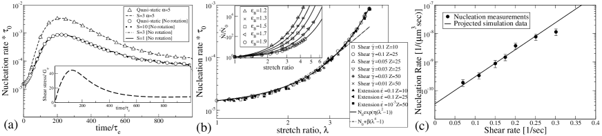
Figure 2: (a) Transient and quasi-static nucleation rates for a $Z=25$ monodisperse melt with $\epsilon_{B}=1.9$ and $\mu_{S}=1.9$ under start-up shear at $\dot{\gamma}\tau_{e}=0.1$; inset contains GLaMM model predictions for shear stress ($G_{e}$ is the shear modulus). (b) Master-curve of nucleation rate against stretch ratio ($\dot{\epsilon}$ is the extension rate); inset shows the master-curves for varying $\epsilon_{B}$. (c) Steady-state nucleation rate measurements against shear rate for an industrial iPP melt Coccorullo et al. (2008) compared with projected simulation results.

We simulate two types of MC moves: addition of a new stem containing one monomer and lengthening of an existing stem by adding a new monomer, each with a corresponding reverse move. As in Jarecki (2007) we assume that to attach, a monomer must be oriented within a solid tolerance angle $\Omega$ of the nucleus orientation. For small $\Omega$, the fraction of monomers within this angle is $w(\theta)\Omega$, where $\theta$ is the angle between the nucleus polar radius and the sub-chain principle strain axis. The stem attachment rate for species $i$ is proportional to its melt concentration $\phi_{i}$. In contrast, for stem lengthening only the next monomer along the chain forming the stem can crystallize. The concentration of this monomer at the nucleus surface where the lengthening event occurs is taken to be unity. Thus the attachment ($+$) and detachment ($-$) move rates for stem addition ($k_{st}$) and stem lengthening ($k_{len}$) are:

$$\begin{array}[]{rr}k^{+}_{st}=\frac{1}{\tau_{0}}\phi_{i}\omega_{i}\mathrm{min}(1,e^{-\Delta\mathcal{F}^{+}_{st}})&k^{-}_{st}=\frac{1}{\tau_{0}}\mathrm{min}(1,e^{-\Delta\mathcal{F}^{-}_{st}})\\ k^{+}_{len}=\frac{1}{\tau_{0}}\omega_{i}\mathrm{min}(1,e^{-\Delta\mathcal{F}^{+}_{len}})&k^{-}_{len}=\frac{1}{\tau_{0}}\mathrm{min}(1,e^{-\Delta\mathcal{F}^{-}_{len}})\end{array}$$

where $\tau_{0}$ is the time for a monomer attachment attempt, $\omega_{i}=4\pi w_{i}(\theta_{i})$ is the fraction of correctly aligned monomers (normalized to unity in the quiescent limit), and the constant $\ln(\Omega/4\pi)$ has been added to $\epsilon_{B}$. The free energy change of attaching a new stem of species $i$ is

$$\begin{array}[]{c}\Delta\mathcal{F}^{+}_{st}=\mathcal{F}(N_{T}+1,N_{s}+1)-\mathcal{F}(N_{T},N_{s})-\frac{1}{N_{e}}\Delta F^{el}_{i}(\mathbf{f}_{i}),\end{array}$$

where $\Delta F^{el}_{i}$ is the flow-induced free energy change in sub-chain $i$. Similar calculations give the free energy changes for the other move types. A stem can only be detached if it contains a single monomer.

The kinetic MC algorithm requires a sum over all possible move rates. The area available for stem addition moves is $\mathcal{A}(N_{s})$, which is taken to be proportional to $\sqrt{N_{s}}$, and to give spherical nuclei in the quiescent limit. To obey detailed balance the rate of stem removal must be multiplied by $\mathcal{A}(N_{s}-1)/N_{s}$, the probability of a given stem being at the nucleus surface. Each stem can lengthen or shorten from either the top of bottom. Thus the total sum over all possible move rates is:

$$\begin{split}K_{\mathrm{Total}}&=\mathcal{A}(N_{s})\sum_{i=1}^{Z}(k^{+}_{st})_{i}+\frac{\mathcal{A}(N_{s}-1)}{N_{s}}\sum_{j=1}^{N_{s}}(k^{-}_{st})_{j}\\ &+\sum_{j=1}^{N_{s}}\Big{(}(k_{len}^{+top})_{j}+(k_{len}^{-top})_{j}+(k_{len}^{+bot})_{j}+(k_{len}^{-bot})_{j}\Big{)}.\end{split}$$

At each kinetic MC timestep one move is performed at random, with the selection probability weighted by the move rate. Time is then incremented by a stochastically determined interval $\Delta t=-\ln\zeta/K_{Total}$, where $\zeta$ is chosen uniformly on $[0,1]$ Gillespie (1977); Doye and Frenkel (1998).

After each MC step the nucleus orientation $\hat{\mathbf{v}}$ is incremented over $\Delta t$ by Brownian dynamics. Flow rotates the spheroid nucleus through the Jeffery algorithm Leal and Hinch (1971). The angular diffusion time $\tau_{rot}$ scales with both the nucleus volume $N_{T}$ and aspect ratio $\rho$ following the expressions in Leal and Hinch (1971), giving $\tau_{rot}=\alpha\tau_{0}N_{T}G(\rho)$, where $G(\rho)$ depends only on the aspect ratio and we have introduced a dimensionless constant $\alpha$, connecting $\tau_{rot}$ with the monomer attachment time $\tau_{0}$. As the Jeffery algorithm is for Newtonian fluids we have neglected non-Newtonian effects here. After each time step all $\mathbf{f}_{i}$ values are updated from the GLaMM model results, and $\Delta F^{el}_{i}$ and $\omega_{i}$ are recalculated. The parameter $\mathcal{S}=\tau_{e}/\tau_{0}$ sets the ratio of flow and monomer attachment timescales. We use $\mathcal{S}=10$ throughout this Letter, unless indicated otherwise, although similar results are obtained for any value of $\mathcal{S}>1$.

III Results

Each simulation evolves a single nucleus from a single monomer. The algorithm is especially effective at low undercooling, as for small nuclei the rate sum is small, leading to large time steps. The quiescent free energy landscape can be calculated analytically from $\epsilon_{B}$ and $\mu_{S}$ to give a dimensionless nucleation barrier $\Delta f^{*}$ and a critical nucleus of $n^{*}$ monomers. The simulated nucleation time $\tau_{N}$ is the first time the polar and equatorial radii simultaneously exceed the critical radius $r^{*}=\sqrt[3]{3n^{*}/4\pi}$. Choosing a larger threshold size for nucleation has little effect on $\left<\tau_{N}\right>$. The results are accurately approximated by $\left<\tau_{N}\right>=\tau_{0}\exp(\Delta f^{*})$. We obtained good statistics for barriers up to $25k_{B}T$ in $\sim 50$hrs on one $2$GHz processor, giving a nucleation time of $\sim 10^{11}\tau_{0}$. The nucleation times are Poisson distributed, so the nucleation rate can be defined as $\dot{N}_{0}=1/\left<\tau_{N}\right>$.

Under flow, the nucleation kinetics depend on the evolving chain deformation. We define the instantaneous nucleation rate $\dot{N}(t)\approx\frac{1}{1-n(t)}\frac{n(t+\Delta t)-n(t-\Delta t)}{2\Delta t}$ where $n(t)$ is the cumulative fraction of runs nucleated at time $t$. For shear rates $\dot{\gamma}$ that are slow compared to the critical nucleus rotation time ($\tau_{rot}^{n^{*}}\dot{\gamma}\ll 1$) alignment effects can be ignored, equivalent to taking $\alpha=0$. The GLaMM model predictions for start-up of constant shear at $\dot{\gamma}\tau_{e}=0.1$ of a $Z=25$ melt and the resulting instantaneous nucleation rate are in fig 2(a). The results are independent of the ratio of flow and crystallization timescales for $\mathcal{S}\gtrsim 1$. In fact, fixing the non-crystalline chain configuration to that corresponding to flow time $t$ for the entire simulation and plotting the resulting quasi-static nucleation rate against $t$, reproduces the transient results (fig 2a). Thus nucleation is fully controlled by the instantaneous configuration of the surrounding chains, if $\tau_{e}>\tau_{0}$.

The stretch ratio $\lambda=\frac{1}{Z}\sum_{i=1}^{Z}\sqrt{\left<\mathbf{r}_{i}^{2}\right>}$ is the dominant factor determining the nucleation rate, despite variations in flow rate, molecular weight and flow geometry (Fig 2(b)). This universal result is somewhat surprising as the distribution of stretch along the chain varies considerably with flow conditions, which may be expected to influence nucleation, especially if molecular weight and flow geometry is varied. This result will be useful in deriving simple differential models of FIC Zuidema et al. (2001); Steenbakkers et al. (2008) as the nucleation rate can be described the expression $\dot{N}=\dot{N}_{0}\exp(\eta(\lambda^{2}-1))$, where $\eta$ is a fitting constant. Also in fig 2(b) is the curve $\dot{N}=\dot{N}_{0}+\beta(\lambda^{4}-1)$, which empirically fits measured nucleation rates from flowing melts Steenbakkers et al. (2008). The agreement with our simulation data for $\lambda\lesssim 3.5$ theoretically justifies this empirical expression. In the inset to fig 2(b) the sensitivity of nucleation to chain stretching increases with decreased undercooling (decreasing $\epsilon_{B}$), as seen experimentally Coppola et al. (2004). Fig 2(c) directly compares our simulations with steady-state nucleation rate measurements on a polydisperse isotactic polypropylene sample (iPP) during shear Coccorullo et al. (2008). The parameter determination, projection of the simulation to large energy barriers and the approximation of the molecular weight distribution as a bimodal blend are detailed in appendix A. The close agreement shows our model can quantitatively account for FIC measurements. Fig 2(a) also shows the transient nucleation rate when $\alpha=5$. This higher $\alpha$ value gives slower angular diffusion, meaning that flow aligns sub-critical nuclei, accelerating nucleation. Here, the quasi-static nucleation remains Poissonian and matches the transient rates, although $\dot{N}$ now depends on both $\lambda$ and $\dot{\gamma}\tau_{rot}^{n^{*}}$. Further increases of $\alpha$ give almost identical results.

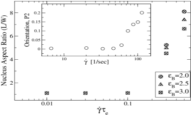
Figure 3: Simulated nucleus aspect ratio at point of nucleation against shear rate for a $2\%$ high molecular weight blend, ($\alpha=5.0$, $\mu_{S}=2.5$, sheared for $120\tau_{e}$); inset shows experimental orientation data on a bimodal blend sheared for $20$ sec Mykhaylyk et al. (2008).

In experiments shish nuclei are especially prevalent in melts of short chains blended with a small amount of very long chains Hsiao et al. (2005); Balzano et al. (2008); Seki et al. (2002); Heeley et al. (2006); Mykhaylyk et al. (2008). We simulated a melt of $Z=15$ chains blended with $2$wt$\%$ of $Z=52$ chains, using a generalization of the GLaMM model to bimodal blends Graham et al. (2009). High shear produces very elongated nuclei (fig 3) from a purely kinetic mechanism. The shish widen by adding new stems using any monomer from the melt, whereas shish lengthen by adding monomers along an existing stem. Therefore the concentration of monomers from stretched segments at the growth surface is greater for lengthening than for widening, provided the nucleus contains a disproportionate number of stretched segments. Fast flow conditions are required for this disparity to overcome the significant surface area cost of elongated nuclei. Fig 3 (inset) shows experimental data for an orientational order parameter, the P2 orientation function, against shear rate for a $2\%$ high molecular weight blend Mykhaylyk et al. (2008), highlighting similarities with our predictions. Also in Fig 3 reduced undercooling, from reducing $\epsilon_{B}$, increases the anisotropy, as seen experimentally Balzano (2008). When crystallization is less favorable, the disparity in the kinetics of stretched and unstretched chain segments increases.

IV Discussion

Our efficient kinetic Monte Carlo algorithm for flow-induced nucleation in polymer melts is tractable even at low undercooling. The flow-induced nucleation rate is a universal function of the chain stretch ratio, independent of flow rate, molecular weight and flow geometry, but with decreasing undercooling causing increased flow sensitivity. This universal curve is very similar to an empirical relationship that accurately describes flow induced nucleation rate measurements Steenbakkers et al. (2008), justifying this empirical result. Our successful quantitative comparison with nucleation measurements Coccorullo et al. (2008) establishes that changes in chain free energy under flow can describe flow enhanced nucleation in semi-crystalline polymers. In our bimodal blend simulations, a few percent of high molecular weight chains optimizes shish formation and the degree of anisotropy increases with shear rate and decreased undercooling, all of which are seen experimentally Hsiao et al. (2005); Balzano et al. (2008); Seki et al. (2002); Heeley et al. (2006); Mykhaylyk et al. (2008); Balzano (2008). The simulation can readily be generalized to fully polydisperse melts, an essential step to model industrial polymer processing. The efficiency and flexibility of our algorithm makes it suitable to simulate general anisotropic nucleation under external fields.

V Acknowledgements

We thank the EPSRC for funding (GR/T11807/01) and L Balzano, R Steenbakkers, G Peters, O Mykhaylyk, T Ryan and T McLeish for useful discussions.

Appendix A Comparison with nucleation measurements.

A.1 Introduction

Here we quantitatively compare our simulation results with directly observed steady-state nucleation rates from a polymer melt under shear Coccorullo et al. (2008). These measurements, by Coccorullo et. al, were made on a commercial grade isotactic polypropylene (iPP), known as iPP T30G. These data show an exponential dependence of the nucleation rate with shear rate, which our model correctly predicts. In order to quantitatively model this system, the required parameters fall into two classes: molecular relaxation times, which can be accurately calculated from literature values; and crystallization parameters, for which order of magnitude estimates are provided by the literature, but whose specific values we determine from the nucleation data. The high polydispersity of iPP T30G is a further complication. As the full molecular weight distribution (MWD) for this resin was not reported, we choose a realistic MWD for highly polydisperse materials and demonstrate that this distribution is consistent with both the reported molecular weight averages and linear rheological measurements. For non-linear flow modeling, we approximate this polydisperse melt as a bimodal blend, since no polydisperse equivalent of the GLaMM mode is currently available. We note that no fundamental modification of our simulation algorithm would be required to take advantage of the results of a polydisperse tube model. In this data comparison we are able to correctly describe these steady state nucleation rate measurements against shear rate, using crystallization parameters that are consistent with estimates provided by literature measurements.

A.2 Molecular relaxation times

The relaxation times of iPP T30G can be determined by the tube model and confirmed against linear oscillatory shear measurements. Taking the tube model parameters for iPP from the literature van Meerveld (2004) and shifting $\tau_{e}$ to the experimental temperature of $140^{\circ}$C using the time-temperature superposition parameters for iPP T30G Coccorullo et al. (2003), gives $\tau_{e}=90$ns and $M_{e}=4.4$kg/mol. Here $\tau_{e}$ is the Rouse time of an entanglement segment and $M_{e}$ is the molecular weight between entanglements. The mass of a Kuhn step of iPP is $187.8$g/mol Langston et al. (2007), meaning the number of Kuhn steps per entanglement segment is $N_{e}\approx 25$. From these parameters the chain Rouse time can be calculated using $\tau_{R}=(M/M_{e})^{2}\tau_{e}$ Doi and Edwards (1986).

The form of the molecular weight distribution (MWD) for iPP T30G is essential to our modeling as small amounts of high molecular weight (HMW) material can control FIC (See, for example, ref Seki et al. (2002)). Unfortunately, the full MWD of iPP T30G was not reported, with only the weight and number average molecular weights being given Coccorullo et al. (2008). Furthermore, standard distribution functions, such as the log-normal and generalized exponential distributions, typically under-estimate the HMW tail of highly polydisperse melts Ruymbeke et al. (2002). Fortunately, linear rheological measurements are highly sensitive to this HMW tail at low frequencies and these data provide a clear upper-bound on the amount of HMW material. Thus we select a realistic form for the full MWD and show that this is consistent with both the reported complex viscosity and molecular weight measurements ($M_{w}=481$kg/mol and $M_{n}=75$kg/mol). We describe the MWD using a bimodal log-normal distribution, since the augmented tail of this distribution accounts more accurately for the HMW tail of highly polydisperse melts than standard monomodal distributions. This takes the form

$$w_{Blend}(m)=(1-\phi_{h})w_{LN}(m,M_{wl},M_{nl})+\phi_{h}w_{LN}(m,M_{wh},M_{nh})$$ (2)

where $\phi_{h}$ is volume fraction of the HMW peak, $M_{wl/h}$ and $M_{nl/h}$ are the weight and number average molecular weights for the low and high molecular weight chains, respectively, and $w_{LN}$ is the monomodal log-normal distribution. Taking $\phi_{h}=0.01\%$, $M_{wh}=3\times 10^{5}$kg/mol, $M_{nh}=2\times 10^{4}$kg/mol, $M_{wl}=451$kg/mol and $M_{nl}=75$kg/mol gives the correct overall weight and number average molecular weights and correctly predicts the complex viscosity measurements. These values were chosen as they correspond to the longest HMW tail that correctly predicts the complex viscosity measurements. Fig 4(a) shows the molecular weight distribution and fig 4(b) compares the predicted complex viscosity resulting from this distribution with measurements on iPP T30G. Here the linear oscillatory shear response was computed using a polydisperse tube model for linear response, which combines the tube escape formula of Likhtman and McLeish Likhtman and McLeish (2002) with the Rubinstein and Colby algorithm for constraint release Rubinstein and Colby (1988) and is implemented within our in-house software for molecular rheology, RepTate . Using a monomodal log-normal distribution, with $\phi_{l}=0$, produces slightly inferior agreement with the complex viscosity measurements and cannot account for the nucleation measurements.

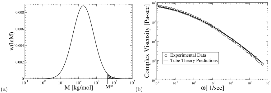
Figure 4: (a) Molecular weight distribution used to model iPP T30G calculated from eqn (2). The shaded area is the region of the molecular weight distribution defined as the high molecular weight tail in our modelling. (b) Linear rheological measurements on iPP T30G Coccorullo et al. (2008) along with the predictions of polydisperse tube model using the molecular weight distribution discussed above and with $G_{e}=1.1\times 10^{6}$Pa).

As discussed above, because there is no suitable polydisperse tube model for non-linear flow, we approximate iPP T30G as a bimodal blend when modelling its non-linear response. Fig 4(a) shows that there is no clear molecular weight at which to define the division between the two blend species. We choose the high molecular weight fraction to be all material with a molecular weight above $M^{*}=4200$kg/mol, giving a HMW volume fraction of $1\%$. Taking a lower value of $M^{*}$ produces a Rouse time that is too short to account for the flow nucleation measurements, but we note that larger values of $M^{*}$ may be equally valid choices. We note also that this fraction contains discernible contributions from both of the monomodal terms in eqn (2). We compute the expectation value of the Rouse time of the high molecular weight tail via,

$$\left<\tau_{R}\right>=\frac{\int_{M^{*}}^{\infty}\tau_{e}(m/M_{e})^{2}w_{Blend}(m)\mathrm{d}m}{\int_{M^{*}}^{\infty}w_{Blend}(m)\mathrm{d}m},$$ (3)

which gives $\tau_{R}=66$sec. All material below $M^{*}$ is defined as matrix material, and a similar calculation gives the average Rouse time of this matrix as $2.1$ms. Thus, the matrix relaxes too quickly to be stretched by the flow rates in the study of Coccorullo et al.. Hence, we model the non-linear flow dynamics of this polydisperse material by approximating it as a bimodal blend with the two fractions having the Rouse times discussed above.

A.3 Crystallization parameters

To model iPP T30G we require its quiescent critical nucleus size and barrier height, at the experimental temperature. An estimate for the number of Kuhn steps in a critical nucleus can be found from literature data. The critical nucleus diameter has been shown to be of the order of the lamella thickness by transmission electron microscopy Bassett and Olley (1984); Olley and Bassett (1989) for iPP and confirmed for a different polymer by atomic force microscopy Li et al. (1999). For iPP the lamella thickness is $\sim 10$nm at $140^{\circ}$C. Using the iPP crystal density of $0.9$g/cm³ Ran et al. (2001) and the Kuhn step mass for iPP Langston et al. (2007) and assuming a spherical critical nucleus gives the number of Kuhn steps in a critical nucleus as $\sim 1000$.

The barrier height can be estimated from the nucleation data of Coccorullo et. al Coccorullo et al. (2008) (see fig 6). Projecting these data to zero shear rate gives a quiescent homogeneous nucleation rate of $3.4\times 10^{-11}/\mu$m³/sec. This can be converted to a rate per Kuhn step using the melt density of iPP ($0.85$g/cm³) and the iPP Kuhn step mass. Thus the density of Kuhn steps is $\rho_{K}=2.7\times 10^{9}/\mu$m³ so the quiescent nucleation rate is $\dot{N}_{0}=1.2\times 10^{-20}$/sec per Kuhn step. Taking the crystallization timescale of a Kuhn step $\tau_{0}$ to be of the order of the Kuhn step relaxation time $\tau_{K}=\tau_{e}/N_{e}^{2}=0.144$ns, means that $\dot{N}_{0}\tau_{0}\sim 10^{-30}$. Clearly nucleation in this system is extremely rare and such a separation of timescales cannot feasibly be simulated even by our highly efficient kMC algorithm. Instead we systematically project our results to larger energy barriers to allow a comparison with these data.

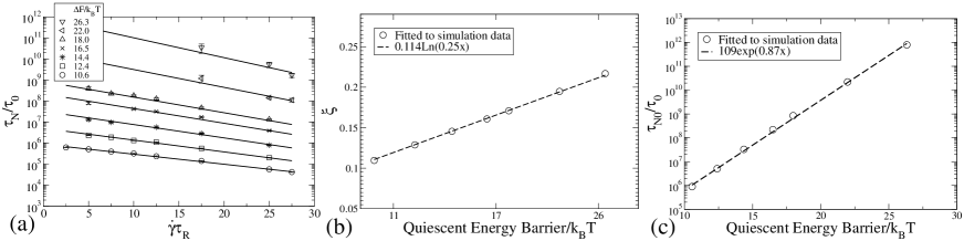
Figure 5: Projection of the simulated nucleation data to large energy barriers: (a) Simulation data for the average steady shear nucleation time against shear rate for a HMW volume fraction of $1\%$ fitted with eqn (4) [shapes are simulation data and lines are fits]; (b) Variation of the sensitivity of the nucleation time to shear rate with quiescent barrier height; (c) Variation of $\tau_{0}$ with quiescent barrier height.

A.4 Projection to large nucleation barriers

To perform this projection we simulated the average nucleation time over a range of quiescent nucleation barrier heights, varying from $10.6$ to $26.3\mathrm{k_{B}T}$, with the critical nucleus size held fixed at $1081$ Kuhn steps. Nucleus alignment was neglected for all of these simulations ($\alpha=0$, throughout). The steady-state configuration for both blend components for various shear rates was calculated using a recent generalisation of the GLaMM model to bimodal blends Graham et al. (2009). The dimensionless steady-state nucleation time $\tilde{\tau}_{N}=\tau_{N}/\tau_{0}$ against shear rate $\dot{\gamma}$ was simulated using the GLaMM model predictions, in steady state, for a range of shear rates and molecular weights. The results are independent of molecular weight when the shear rate is expressed as a Rouse Weissenberg number $\dot{\gamma}\tau_{R}$, but do depend on the height of the quiescent nucleation barrier, $\Delta f^{*}$, as shown in figure 5(a). The simulated nucleation times vary exponentially with shear rate and can be described by the expression

$$\tilde{\tau}_{N}(\dot{\gamma})=\tilde{\tau}_{N0}\exp(-\xi\dot{\gamma}\tau_{R}),$$ (4)

where $\tilde{\tau}_{N0}$ and $\xi$ are fitting parameters characterizing the decay of the nucleation time with shear rate, both of which depend on the barrier height $\Delta f^{*}$. The lines in fig 5(a) are the result of fitting eqn (4) to the simulation data. Both of the fitting parameters have a simple dependence on $\Delta f^{*}$, as shown in figs 5(b) and (c). Data for to the two largest quiescent barriers was used only to confirm the projection and was not involved in the fitting. This procedure allows the simulation results to be projected to nucleation barriers that are too high to be simulated.

A.5 Data comparison

We can use our projected results to model the data of Coccorullo et. al Coccorullo et al. (2008). The value of the projected zero shear nucleation rate from these data, combined with the projection formula in fig 5(c) and the requirement that $\tau_{0}\sim\tau_{K}$, gives a quiescent nucleation barrier of $\Delta f^{*}\sim 70\mathrm{k_{B}T}$. The final value of $f^{*}$ is chosen to reproduce the slope of the experimental data in figure 6. Thus, using the Rouse time computed above and taking a value of $\Delta f^{*}=72\mathrm{k_{B}T}$ gives $\xi=0.33$ from the projection formula in figure 5(b). This quiescent barrier specifies $\tilde{\tau}_{N0}=1.74\times 10^{29}$ by the projection formula in figure 5(c). Thus taking $\tau_{0}=0.46$ns produces agreement with the experimental data in fig 6 extrapolated to zero shear rate. We can also confirm that this value for $\tau_{0}$ is $\sim\tau_{K}$. With these parameters and using $\dot{N}(\dot{\gamma})=1/\tau_{N}(\dot{\gamma})$, which is valid because all of the simulated nucleation processes are Poissonian, eqn (4) can be written as

$$\dot{N}(\dot{\gamma})=\frac{\rho_{K}}{\tilde{\tau}_{N0}\tau_{0}}\exp(\xi\dot{\gamma}\tau_{R})=3.4\times 10^{-11}\exp(21.8\mathrm{sec}\dot{\gamma})/\mathrm{sec}/\mu\mathrm{m}^{3}.$$ (5)

Eqn (5) produces the projected simulation data in fig 6.

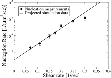
Figure 6: Comparison of measured steady shear nucleation rate against shear rate for an iPP resin Coccorullo et al. (2008) with our projected simulation results.

In summary, our model correctly predicts the exponential dependence of nucleation rate on shear rate as observed by Coccorullo et al. Coccorullo et al. (2008). Furthermore, with a characterization of the full molecular weight distribution and extrapolation of our simulation results to high nucleation barriers, we can make a direct quantitative comparison with these data. We use crystallization parameters that are estimated from the literature but whose final values are determined in response to the nucleation data. This results in very good agreement with directly measured nucleation rates under flow using parameters that are consistent with literature estimates.

Several consequences arise from this data comparison. It demonstrates that changes in chain free energy upon stretching under flow are sufficient to quantitatively account for the degree of enhanced nucleation measured in flowing semi-crystalline polymers. It also indicates the strong need for comprehensive material characterization to accompany FIC measurements. In particular, an accurate characterization of the sample’s high molecular weight tail, along with linear rheological modeling, will clearly define the full spectrum of molecular relaxation times. The issues of polydispersity could be solved either through FIC experiments on model polymers or through the emergence of a reliable non-linear flow model for polydisperse polymers. In principle, our model can predict the effect of varying molecular weight distribution, temperature and flow history, including transient flows, and a more comprehensive test of the model’s predictions could be produced by systematic comparison to such a data set. The close agreement between theory and experimental data and our comparison provides a foundation on which further quantitative comparisons can be built.

References

- Keller and Kolnaar (1997) A. Keller and H. W. Kolnaar, in Processing of Polymers, edited by H. Meijer (Wiley, Weinheim, 1997).
- Binsbergen (1966) F. L. Binsbergen, Nature 211, 516 (1966).
- Kimata et al. (2007) S. Kimata et al., Science 316, 1014 (2007).
- Hsiao et al. (2005) B. S. Hsiao et al., Phys. Rev. Lett. 94, 117802 (2005).
- Balzano et al. (2008) L. Balzano et al., Phys. Rev. Lett. 100, 048302 (2008).
- Seki et al. (2002) M. Seki et al., Macromolecules 35, 2583 (2002).
- Heeley et al. (2006) E. L. Heeley et al., Macromolecules 39, 5058 (2006).
- Mykhaylyk et al. (2008) O. O. Mykhaylyk et al., Macromolecules 41, 1901 (2008).
- Waheed et al. (2005) N. Waheed, M. J. Ko, and G. C. Rutledge, Polymer 46, 8689 (2005).
- Hu et al. (2002) W. Hu, D. Frenkel, and V. Mathot, Macromolecules 35, 7172 (2002).
- Zhang and Muthukumar (2007) J. Zhang and M. Muthukumar, J. Chem. Phys. 126, 234904 (2007).
- Eder and Janeschitz-Kriegl (1997) G. Eder and H. Janeschitz-Kriegl, in Processing of Polymers, edited by H. E. H. Meijer (Wiley, Weinheim, 1997).
- Zuidema et al. (2001) H. Zuidema, G. W. M. Peters, and H. E. H. Meijer, Macromol. Theor. Simul. 10, 447 (2001).
- Steenbakkers et al. (2008) R. J. A. Steenbakkers, G. W. M. Peters, and H. E. H. Meijer, in The XV International Congress On Rheology: The Society of Rheology 80th Annual Meeting (2008), vol. 1027 of AIP Conference Proceedings, pp. 493–495.
- Coppola et al. (2001) S. Coppola, N. Grizzuti, and P. L. Maffettone, Macromolecules 34, 5030 (2001).
- Kulkarni and Beris (1999) J. Kulkarni and A. Beris, Journal of Non-Newtonian Fluid Mechanics 82, 331 (1999).
- Gillespie (1977) D. T. Gillespie, J Phys Chem 81, 2340 (1977).
- Graham et al. (2003) R. S. Graham et al., J. Rheol. 47, 1171 (2003).
- Bent et al. (2003) J. Bent et al., Science 301, 1691 (2003).
- Blanchard et al. (2005) A. Blanchard et al., Phys. Rev. Lett. 95, 166001 (2005).
- Doye and Frenkel (1998) J. Doye and D. Frenkel, Phys Rev Lett 81, 2160 (1998).
- Cohen (1991) A. Cohen, Rheologica Acta 30, 270 (1991).
- Olmsted and Milner (1994) P. D. Olmsted and S. T. Milner, Macromolecules 27, 6648 (1994).
- Jarecki (2007) L. Jarecki, in Progress in Understanding of Polymer Crystallization, edited by G. Reiter and G. R. Strobl (Springer, Berlin, 2007), vol. 714, p. 65.
- Coccorullo et al. (2008) I. Coccorullo, R. Pantani, and G. Titomanlio, Macromolecules 41, 9214 (2008).
- Leal and Hinch (1971) L. G. Leal and E. J. Hinch, J Fluid Mech 46, 685 (1971).
- Coppola et al. (2004) S. Coppola et al., Polymer 45, 3249 (2004).
- Graham et al. (2009) R. S. Graham et al., Soft Matter 5, 2383 (2009).
- Balzano (2008) L. Balzano, Ph.D. thesis, TU/e (Eindhoven) (2008).
- van Meerveld (2004) J. van Meerveld, Rheol Acta 43, 615 (2004).
- Coccorullo et al. (2003) I. Coccorullo, R. Pantani, and G. Titomanlio, Polymer 44, 307 (2003).
- Langston et al. (2007) J. A. Langston, R. H. Colby, T. C. M. Chung, F. Shimizu, T. Suzuki, and M. Aoki, Macromolecules 40, 2712 (2007).
- Doi and Edwards (1986) M. Doi and S. F. Edwards, The Theory of Polymer Dynamics (Oxford University Press, Oxford, 1986).
- Ruymbeke et al. (2002) E. V. Ruymbeke, R. Keunings, and C. Bailly, Journal of Non-Newtonian Fluid Mechanics 105, 153 (2002).
- Likhtman and McLeish (2002) A. E. Likhtman and T. C. B. McLeish, Macromolecules 35, 6332 (2002).
- Rubinstein and Colby (1988) M. Rubinstein and R. H. Colby, J. Chem. Phys. 89, 5291 (1988).
- Bassett and Olley (1984) D. C. Bassett and R. H. Olley, Polymer 25, 935 (1984).
- Olley and Bassett (1989) R. Olley and D. Bassett, Polymer 30, 399 (1989).
- Li et al. (1999) L. Li, C. M. Chan, J. X. Li, K. Ng, K. L. Yeung, and L. T. Weng, Macromolecules 32, 8240 (1999).
- Ran et al. (2001) S. Ran, X. Zong, D. Fang, B. S. Hsiao, B. Chu, and R. A. Phillips, Macromolecules 34, 2569 (2001).