Riemann solvers and undercompressive shocks
of convex FPU chains

Abstract

We consider FPU-type atomic chains with general convex potentials. The naive continuum limit in the hyperbolic space-time scaling is the p-system of mass and momentum conservation. We systematically compare Riemann solutions to the p-system with numerical solutions to discrete Riemann problems in FPU chains, and argue that the latter can be described by modified p-system Riemann solvers. We allow the flux to have a turning point, and observe a third type of elementary wave (conservative shocks) in the atomistic simulations. These waves are heteroclinic travelling waves and correspond to non-classical, undercompressive shocks of the p-system. We analyse such shocks for fluxes with one or more turning points.

Depending on the convexity properties of the flux we propose FPU-Riemann solvers. Our numerical simulations confirm that Lax-shocks are replaced by so called dispersive shocks. For convex-concave flux we provide numerical evidence that convex FPU chains follow the p-system in generating conservative shocks that are supersonic. For concave-convex flux, however, the conservative shocks of the p-system are subsonic and do not appear in FPU-Riemann solutions.

1 Introduction

The derivation of effective continuum descriptions for high-dimensional discrete systems is a fundamental tool for model reduction in the sciences. Hamiltonian lattices, such as atomic chains, naturally lead to nonlinear systems of conservation laws which describe the leading order dynamics on the hyperbolic space–time scale. It is customary to neglect the higher order terms and to study the leading order system by itself. The rigorous mathematical validity of this reduction is a notoriously difficult task and there are surprisingly few successes reported in the literature.

This paper concerns the macroscopic description of monoatomic chains with nearest neighbour interactions, see Figure 1.1. In their seminal paper [FPU55] Fermi, Pasta and Ulam chains studied such chains for interaction potential $\Phi$ whose non-harmonic part involves only cubic or quartic terms. We allow for general convex interaction potentials, but still refer to the systems as FPU chains.

Figure 1.1: The atomic chain with nearest neighbour interaction.

An important building block for the macroscopic descriptions of FPU chains are the solutions to Riemann initial data in the hyperbolic continuum limit. In this limit space and time are scaled in the same way, and the amplitude of solutions is unconstrained. Since the numerical study of Holian and Straub [HS78] and from rigorous results for the integrable Toda chain it is known that the solutions to atomistic Riemann problems with either convex or concave flux $\Phi^{\prime}$ obey a self-similar structure on the hyperbolic scale: each solution consists of at most two elementary waves that are separated by constant states. Each of these elementary wave is either a rarefaction wave, in which the atomic data vary smoothly on the macroscopic scale, or a dispersive shocks, in which strong microscopic oscillations spread out in space and time.

The starting point for our investigation was the observation that for certain $\Phi$ a third kind of elementary waves can be observed in FPU-Riemann problems. These waves, which we refer to as conservative shocks, involve no oscillations and look like ‘shocks’ (jump discontinuities) on the macroscopic scale. Of course, these waves are not exact shocks as they exhibit a transition layer on the atomistic scale, but this layer is very small and disappears in the hyperbolic scaling. To our knowledge the appearance of conservative shocks in FPU-Riemann problems was never reported before.

An illustrative example of an FPU-Riemann problem is plotted in Figure 1.2 and involves all types of elementary waves (from left to right): a rarefaction wave, a dispersive shock, and conservative shock.

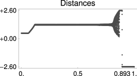
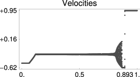
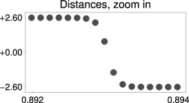
Figure 1.2: Riemann problems in convex FPU chains can involve three kinds of elementary waves: rarefaction waves, dispersive shocks, and conservative shocks. The first two pictures show snapshots of the atomic distances and velocities against the scaled particle index $\alpha/N$ for a chain with $N=8000$ particles and flux $\Phi^{\prime}{\left({r}\right)}=\tfrac{1}{16}{\left({r+\arctan{r}}\right)}$; the third pictures magnifies the region around the conservative shock.

The naive approach to describe the FPU dynamics on the hyperbolic scale assumes long-wave-length motion without microscopic oscillations. Under this assumption one readily derives the ‘p-system’, which consists of the conservation laws for mass and momentum in Lagrangian coordinates.

It is well known, that the naive continuum limits of nonlinear dispersive lattices provide a reasonable macroscopic model as long as the macroscopic fields are smooth, see, e.g., [Lax86, GL88, HL91, HLM94, LL96]. The nonlinearity, however, usually causes shock phenomena, and the naive continuum limit fails in this case. Instead, lattice systems like FPU typically produce dispersive shocks, in which the atoms self-organize into strong microscopic oscillations. On the macroscopic scale such dispersive shocks can be regarded as measure-valued solutions to the naive continuum limit, see (2) in §2.

The formation of dispersive shocks is a characteristic property of Hamiltonian ‘zero dispersion’ limits and a direct consequence of the conservation of energy, see §2. Moreover, it is known from numerical studies and rigorous results for integrable systems, see [GP73, LL83, Ven85, Lax86, Lax91, LLV93, Kam00], that the oscillations in a dispersive shocks are modulated wave trains (period travelling waves). Figure 1.3 presents a typical example of a dispersive shock in FPU chains. At the shock front, where the amplitudes of the oscillations become maximal, the wave trains converge to a supersonic soliton, that is a homoclinic travelling wave.

By combining non-classical hyperbolic theory of the p-system with macroscopic theory, travelling waves and numerical observations of FPU chains we characterise FPU-Riemann solvers for oscillation-free initial data and fluxes with one turning point.

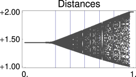
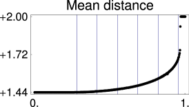
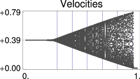
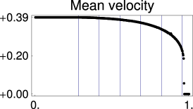
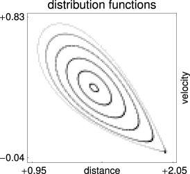
(a)	(b)	(c)

Figure 1.3: Dispersive shocks arise naturally in FPU-Riemann problems as a consequence of energy conservation. Each dispersive shock is build of a one-parameter family of wave trains with a single soliton at the leading front. (a,b) Snapshots of atomic distances and velocities, and their local mean values. (c) Superposition of several local distribution functions within the shock; positions of the mesoscopic space-time windows are marked by vertical lines in (a,b).

Conservative shocks in FPU chains and the p-system.

As shown in Figure 1.2, the solution to FPU-Riemann problems with convex $\Phi$ can involve conservative shocks. Below in §2 we explain that these waves correspond to certain shocks in the p-system, namely those that conserve the energy exactly. Among all p-system shocks, the set of conservative shocks is quite small and if $\Phi^{\prime}$ has no turning point conservative shocks cannot occur at all. The conservative shocks in the p-system are non-classical shocks as they violate the Lax-condition: for convex-concave $\Phi^{\prime}$ there are fast undercompressive, and hence supersonic with respect to both the left and right state; for concave-convex $\Phi^{\prime}$ the conservative shocks are slow undercompressive and hence subsonic.

We numerically discovered that conservative shocks occur naturally in FPU-Riemann problems chains if they are supersonic. However, numerical simulations with concave-convex $\Phi^{\prime}$ never generated anything close to a jump discontinuity. Instead, we typically observe solutions as plotted in Figure 1.4: the solution appears to be a composite wave of a dispersive shock with attached rarefaction wave.

Conservative shocks in FPU chains are naturally related to atomistic fronts which are ‘heteroclinic’ travelling waves. A bifurcation result of Iooss [Ioo00] shows the existence of small amplitude atomistic fronts for convex-concave flux (in which case the conservative shocks are supersonic). The authors have improved this result in [HR09] by showing that each front must correspond to a conservative shock in the p-system and that supersonic shocks with arbitrary large jump height can be realised by an atomistic front.

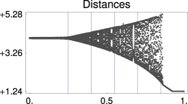
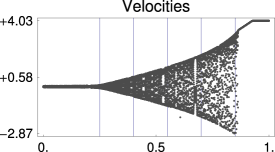
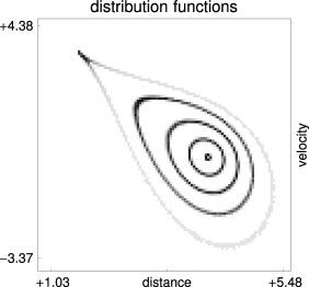
(a)	(b)	(c)

Figure 1.4: FPU-Riemann problem with initial data corresponding to a subsonic conservative shock in the p-system: Instead of a conservative shock the atoms self-organize into a dispersive shock with attached rarefaction wave. The leading soliton in the dispersive shock is hence sonic. (a) atomic distances; (b) atomic velocities; (c) five local distributions functions corresponding to the vertical lines in the snapshots.

FPU-Riemann solvers.

A main goal of this paper is the derivation of FPU-Riemann solvers which predict the number and the type of the elementary waves that result from arbitrary Riemann initial data. To this end we systematically compare numerical simulation for various FPU chains with certain Riemann solvers for the p-system. The FPU-Riemann solver for the Toda chain is well understood, see for instance [Kam93, DM98], but there is no complete picture for non-integrable chains as the available numerical studies only concern special types of Riemann initial data, such as the ‘piston problem’ in [HS78]. Moreover, we are not aware of any previous analytical or numerical investigation of any FPU-Riemann problem which allows for conservative shocks.

In the classical case with either convex or concave flux $\Phi^{\prime}$, the numerical simulations indicate that the solution to each FPU-Riemann problem can be described by an adapted classical solver, in which Lax-shocks are replaced by dispersive shocks. More precisely, from each given left state there emanate four curves (wave sets) in the state space. Two of them correspond to rarefaction waves and appear also in each solver for the p-system. Instead of Lax-shock curves, however, we find two dispersive shock curves. The solution to each FPU-Riemann problem is then completely determined by these wave sets. In particular, in the classical case each Riemann solution consists (generically) of a left moving $1$-wave and a right moving $2$-wave, where each wave is either a rarefaction wave or a dispersive shock.

In presence of turning points of $\Phi^{\prime}$ the Riemann solvers for both FPU chains and the p-system are more complicated because now the solutions to general Riemann problems involve composite waves, which consist of two elementary waves from the same family, and may also involve undercompressive shocks. The Riemann solvers in these cases can be described in terms of modified wave sets, but for the p-system they are not unique. Consequently, different p-system Riemann solvers are possible, such as the ‘conservative’ and the ‘dissipative’ solver described in §4. For FPU chains, however, the underlying atomistic dynamics determines the solver uniquely for each $\Phi$.

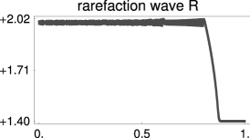
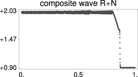
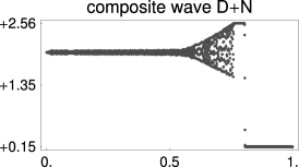
Figure 1.5: Sketch of the modified rarefaction curve ($r_{\mathrm{R}}\leq{r_{\mathrm{L}}}$) for convex-concave $\Phi^{\prime}$ and given $r_{\mathrm{L}}$, and corresponding FPU-Riemann solutions: For $r_{\mathrm{R}}\lesssim{r}_{\mathrm{L}}$ one still finds a rarefaction wave (R), but if $r_{\mathrm{L}}$ crosses the turning point $r_{*}$ of $\Phi^{\prime}$ a non-classical, a conservative shock (N) nucleates. If $r_{\mathrm{R}}$ decreases further the rarefaction wave is replaced by a dispersive shock (D).

In §4 we investigate systematically numerical solutions to FPU-Riemann problems with convex-concave and concave-convex $\Phi^{\prime}$ and argue that the solutions can be described by adapted p-system solvers. More precisely, in the convex-concave we propose to adapt the conservative solver, which predicts composite waves with supersonic conservative shocks. The modified rarefaction curve of such a solver is illustrated in Figure 1.5. In the concave-convex case, however, the simulations indicate that FPU-Riemann solutions can be described by an adapted dissipative solver, whose modified wave sets do not involve conservative shocks. In both non-classical FPU solvers the Lax shocks are replaced by dispersive shocks, and in the nucleation criterion for composite waves the dispersive shock front velocity plays the role of the Rankine-Hugeniot condition. These adaption rules lead to an adequate description of the numerical solution to FPU-Riemann problems. Moreover, the difference between Rankine-Hugeniot and dispersive shock front velocity provides an explanation for the absence of conservation shock in the concave-convex case: the nucleation criterion for conservative shocks cannot be satisfied. However, it is not known how to predict the shock front velocity from the initial data.

We believe that these results give new structural insight into the hyperbolic nature of the continuum limit and the role of the p-system in it. Moreover, they open up new avenues for analytical investigation, some of which we phrase in the form of conjectures.

We emphasize that the situation dramatically changes for fluxes with more than one turning point. On the p-system level, non-classical Riemann solvers can still be constructed, but these no longer provide a basis for the continuum limit of the FPU chain. The reason is that we numerically find energy conserving shocks between wave trains. This is a new phenomenon but its study is beyond the scope of this article. Another problem left for future investigation concerns Riemann problems where oscillations in form of wave trains are already imposed in the initial data. One of the expected new phenomena in this case is the onset of two-phase oscillations. Finally, it would be interesting to study cold initial data with more than one jump discontinuity, because then two-phase oscillations can be created by the interaction of two dispersive shocks.

Organisation of the paper.

In §2 we collect some facts about FPU chains and the p-system; we especially discuss how oscillatory FPU data give rise to measure-valued solutions to the p-systems and briefly outline the concept of modulated wave trains. §3 concerns the numerical simulation of FPU-Riemann problems and contains our observations about self-similarity on the macroscopic scale; we also investigate the fine-structure of dispersive and conservative shocks. §4 is devoted to FPU-Riemann problems. We start with numerical results for the classical case with either convex or concave $\Phi^{\prime}$. Afterwards we discuss the conservative and dissipative solvers for the p-system, and proceed with FPU-Riemann problems in the non-classical cases. Finally, in §5 we prove some analytical results about conservative shocks in the p-system.

2 Preliminaries of FPU chains and the p-system

Convex FPU chains consist of $N$ identical particles which are nearest neighbour coupled in a convex potential $\Phi:\mathbb{R}\to\mathbb{R}$ by Newton’s equations

$$\ddot{x}_{\alpha}=\Phi^{\prime}(x_{\alpha+1}-x_{\alpha})-\Phi^{\prime}(x_{\alpha}-x_{\alpha-1}),$$ (2.1)

where $\dot{~{}}=\frac{\mathrm{d}}{\mathrm{d}t}$ is the time derivative, $x_{\alpha}(t)$ the atomic position, $\alpha=1,\ldots,N$ the particle index. We consider nonlinear force $\Phi^{\prime}$, referred to as the flux. A prominent example for nonlinear $\Phi^{\prime}$ (without turning points) is the completely integrable Toda chain, see [Tod70, Fla74, Hén74], with

$$\Phi_{\mathrm{Toda}}(r)=\exp{\left({1-r}\right)}-(1-r).$$ (2.2)

For our purposes it is convenient to use the atomic distances $r_{\alpha}=\frac{x_{\alpha+1}-x_{\alpha}}{(\alpha+1)-\alpha}$ and velocities $v_{\alpha}=\dot{x}_{\alpha}$ as the basic variables, changing (2.1) to the system

$$\dot{r}_{\alpha}=v_{\alpha+1}-v_{\alpha}\;,\quad\dot{v}_{\alpha}=\Phi^{\prime}{\left({r_{\alpha}}\right)}-\Phi^{\prime}{\left({r_{\alpha-1}}\right)}.$$ (2.3)

Note that while the Toda potential, and also the potentials used below, allows for negative distances, this is essentially a matter of suitably shifting the minimum by $\Phi\to\Phi(\cdot+r_{0})$.

We are interested in the thermodynamic limit $\varepsilon=1/N\to 0$ in the hyperbolic scaling of the microscopic coordinates $t$ and $\alpha$. This scaling is defined by the macroscopic time $\overline{t}=\varepsilon t$ and particle index $\overline{\alpha}=\varepsilon\alpha$. It is natural to scale the atomic positions in the same way, i.e. $\overline{x}=\varepsilon x$, which leaves atomic distances and velocities scale invariant. In the limit $\varepsilon=0$ the spatial variable $\overline{\alpha}$ becomes continuous and the high dimensional ODE (2.1) should be replaced by a continuum limit, i.e., by a system of a few macroscopic PDEs. Microscopic oscillations can be naturally interpreted as a form of temperature in the chain, see [DHR06], and accordingly we refer to oscillation-free limits as cold.

Evolution of cold data and the p-system

To derive the p-system as the simplest model for the macroscopic evolution of FPU chains we assume macroscopic fields $r(\overline{t},\overline{\alpha})$ and $v(\overline{t},\overline{\alpha})$ such that $r_{\alpha}{\left({t}\right)}=r{\left({\varepsilon t},\,{\varepsilon\alpha}\right)}$, $v_{\alpha}{\left({t}\right)}=v{\left({\varepsilon t},\,{\varepsilon\alpha}\right)}$. This ansatz corresponds to cold motion as it assumes that there are no microscopic oscillations in the chain. Substitution into (2.3) and taking the limit $\varepsilon\rightarrow 0$ yields the macroscopic conservation laws for mass and momentum

$$\partial_{\,\overline{t}\,}{r}-\partial_{\,\overline{\alpha}\,}{v}=0,\quad\partial_{\,\overline{t}\,}{v}-\partial_{\,\overline{\alpha}\,}{\Phi^{\prime}{\left({r}\right)}} =0.$$ (2.4)

It is well known that the p-system is hyperbolic for convex $\Phi$ and that for smooth solutions the energy is conserved via

$$\partial_{\,\overline{t}\,}{}{\left({\textstyle{\frac{1}{2}v^{2}}+\Phi{\left({r}\right)}}\right)}-\partial_{\,\overline{\alpha}\,}{}{\left({v\,\Phi^{\prime}{\left({r}\right)}}\right)}=0.$$

In the p-system a shock propagates with a constant shock speed $c_{\mathrm{rh}}$ so that $r$ and $v$ satisfy the Rankine-Hugeniot jump conditions for mass and momentum

$$c_{\mathrm{rh}}{|\![r]\!|}+{|\![v]\!|}=0,\quad c_{\mathrm{rh}}{|\![v]\!|}+{|\![\Phi^{\prime}{\left({r}\right)}]\!|}=0,$$ (2.5)

where ${|\![x]\!|}=x_{\mathrm{L}}-x_{\mathrm{R}}$ denotes the jump. The main observation is that for either convex or concave flux $\Phi^{\prime}$ the jump conditions (2.5) imply that the jump condition for the energy must be violated, i.e.,

$$c_{\mathrm{rh}}{|\![\tfrac{1}{2}v^{2}+\Phi{\left({r}\right)}]\!|}+{|\![v\,\Phi^{\prime}{\left({r}\right)}]\!|}\neq 0,$$ (2.6)

see Theorem 5.1 below. Here the Lax criterion selects the shocks with negative production.

Onset of dispersive shocks in FPU chains

It is known that the p-system provides a reasonable thermodynamic limit for FPU chains in the following sense: Preparing cold FPU initial data with smooth profile functions $r$ and $v$, the atomistic dynamics reproduces a solution to the p-system provided that the latter has a smooth solution. This can be understood as a manifestation of Strang’s Theorem [Str64]; we refer to [DH08] for numerical simulations and to [GL88, HL91] for a similar discussion in the context of other lattice systems.

At some critical time, however, the p-system forms a shock; this shock still conserves mass and momentum according to (2.5), but in most cases it has a negative energy production. In contrast, Newton’s equations always conserve mass, momentum and energy, so the continuum limit of FPU chains beyond a shock cannot be described in terms of the p-system. Instead, the FPU chain produces a dispersive shock with strong microscopic oscillations that take the form of modulated wave trains, compare Observations 3.2 and 3.3 below.

Heuristically, the onset of dispersive shocks is a consequence of energy conservation and can be interpreted as Hamiltonian self-thermalisation: When the shock is formed the p-system predicts some macroscopic excess energy which no longer can be stored in cold motion. On the atomistic scale this excess energy is transferred into modulated wave trains and appears as internal or thermal energy on the macroscopic scale. More precisely, although wave trains do not provide a thermalization in the usual ‘chaotic’ sense, their macroscopic dynamics is governed by thermodynamically consistent field equations, see [DHM06, DHR06].

Riemann solvers for the p-system

The p-system is hyperbolic if $\Phi$ is convex and genuinely nonlinear for $\Phi^{\prime\prime\prime}\neq 0$, thus turning points of $\Phi^{\prime}$ correspond to states in which the system is linearly degenerate. The Riemann problem for strictly convex or concave flux $\Phi^{\prime}$ can therefore be described by the classical solver, which is based on the classical Lax theory from [Lax57] and involves only rarefaction wave and Lax shocks.

This classical Riemann solver is built from the following curves, where $-$ corresponds to left moving $1$-waves and $+$ to right moving $2$-waves. The rarefaction wave sets $\mathcal{R}_{\pm}[u_{{\mathrm{L}}}]$ contain all right states $u_{{\mathrm{R}}}={\left({r_{{\mathrm{R}}}},\,{v_{{\mathrm{R}}}}\right)}$ that can be reached from a given left state $u_{{\mathrm{L}}}={\left({r_{{\mathrm{L}}}},\,{v_{{\mathrm{L}}}}\right)}$ with a single $1$- or $2$-rarefaction wave. The shock wave sets $\mathcal{S}_{\pm}[u_{{\mathrm{L}}}]$ consist of all possible right states $u_{\mathrm{R}}$ that can be reached by a single Lax $1$- or $2$-shock. The sets $\mathcal{W}_{\pm}[u_{{\mathrm{L}}}]=\mathcal{R}_{\pm}[u_{{\mathrm{L}}}]\cup\mathcal{S}_{\pm}[u_{{\mathrm{L}}}]$ form $C^{2}$-smooth curves through $u_{{\mathrm{L}}}$, and we denote $\mathcal{W}[u_{{\mathrm{L}}}]=\mathcal{W}_{-}[u_{{\mathrm{L}}}]\cup\mathcal{W}_{+}[u_{{\mathrm{L}}}]$. The solution to the Riemann problem with given left and right states $u_{\mathrm{L}}$ and $u_{\mathrm{R}}$ consists of the two elementary waves that connect $u_{\mathrm{L}}$ to $u_{\mathrm{M}}$, and $u_{\mathrm{M}}$ to $u_{\mathrm{R}}$ (one of these may be trivial), where the intermediate state is uniquely determined by $u_{\mathrm{M}}\in\mathcal{W}_{-}[u_{\mathrm{L}}]$ and $u_{\mathrm{R}}\in\mathcal{W}_{+}[u_{\mathrm{M}}]$.

In Appendix A we give more details about the classical-solver for the p-system. If $\Phi^{\prime}$ has turning points the wave sets of the classical solver must be modified, and this gives rise to non-classical solvers which involve various types of composite waves, see §4.2.

Conservative shocks in the p-system

In contrast to Lax shocks, conservative shocks in the p-system balance mass, momentum (2.5) and energy (2.6). This gives rise to the system of nonlinear equations

$$\begin{split}c_{\mathrm{rh}}{|\![r]\!|}+{|\![v]\!|}=0,\qquad c_{\mathrm{rh}}{|\![v]\!|}+{|\![\Phi^{\prime}(r)]\!|}=0,\qquad c_{\mathrm{rh}}{|\![\tfrac{1}{2}v^{2}+\Phi{\left({r}\right)}]\!|}+{|\![v\Phi^{\prime}(r)]\!|}=0,\end{split}$$ (2.7)

for the five parameters $r_{\mathrm{L}}$, $v_{\mathrm{L}}$, $r_{\mathrm{R}}$, $v_{\mathrm{R}}$, $c_{\mathrm{rh}}$. According to Appendix A a conservative shock is called supersonic if $|c_{\mathrm{rh}}|>\max\{|\lambda_{\pm}(r_{\mathrm{L}})|,|\lambda_{\pm}(r_{\mathrm{R}})|\}$ and subsonic if $|c_{\mathrm{rh}}|<\min\{|\lambda_{\pm}(r_{\mathrm{L}})|,|\lambda_{\pm}(r_{\mathrm{R}})|\}$. It can be easily shown that each conservative shock satisfies

$$\mathcal{J}(r_{\mathrm{L}},r_{\mathrm{R}}):={|\![\Phi(r)]\!|}-{|\![r]\!|}\langle{\Phi^{\prime}(r)}\rangle=0,\qquad\langle{\Phi^{\prime}(r)}\rangle:=\frac{1}{2}(\Phi^{\prime}(r_{\mathrm{L}})+\Phi^{\prime}(r_{\mathrm{R}})).$$ (2.8)

Conversely, for each solution to (2.8) there exist both a corresponding conservative $1$-shock and $2$-shock. These shocks are unique up to Galilean transformations, and differ only in $\mathrm{sgn}{|\![v]\!|}=\mathrm{sgn}\,{c_{\mathrm{rh}}}$. We analyse the set of conservative shocks in the p-system in more detail in §5.

Macroscopic limit and Young measures

About the hyperbolic continuum limit of FPU chains in the presence of strong microscopic oscillations little is known rigorously. This is the reason why, for a large part, we have to rely on numerical observations. The main difficulty lies in the control of oscillations that lead to measure-valued solutions on the macroscopic scale. Heuristically, such measure-valued solutions are governed by extended p-systems, but a rigorous derivation of such extensions could be treated in a satisfactory manner only for integrable systems so far; notably the harmonic chain [DHM06, Mie06, Mac02, Mac04], the hard sphere model [Her05], and the Toda chain [DKKZ96, DM98].

Nevertheless, some insight into the macroscopic evolution of microscopic oscillations can be gained from the theory of Young measures. Here it is supposed that the atomic data generate a family of probability distributions $\mu{\left({\overline{t}},\,{\overline{\alpha}},\,{\,\mathrm{d}Q}\right)}$, where ${\left({\overline{t}},\,{\overline{\alpha}}\right)}$ is a point in the macroscopic space-time and $Q={\left({r},\,{v}\right)}$ denotes a point in the microscopic phase space of distances and velocities. Note that the atomic data are oscillation free in the vicinity of a point ${\left({\overline{t}},\,{\overline{\alpha}}\right)}$ if and only if the measure $\mu{\left({\overline{t}},\,{\overline{\alpha}},\,{\,\mathrm{d}Q}\right)}$ is a delta distribution with respect to the $Q$ variable.

On the one hand, Young measures provide an elegant framework to investigate oscillatory numerical data that we used to interpret our simulations. For given ${\left({\overline{t}},\,{\overline{\alpha}}\right)}$ the measure $\mu{\left({\overline{t}},\,{\overline{\alpha}},\,{\,\mathrm{d}Q}\right)}$ can be approximated by means of mesoscopic space-time windows and provides local mean values of atomic observables as well as statistical information about the microscopic oscillations, see [DHM06, DH08].

On the other hand, Young measures are useful for analytical considerations because the solutions to (2.1) with $N\to\infty$ are compact in the sense of Young-measures provided that the initial data are of order $1$. Extracting convergent subsequences, one can then prove as in [Her05] that every limit measure must be a weak solution to the following macroscopic conservation laws of mass, momentum and energy

$$\partial_{\,\overline{t}\,}{}{\left\langle r\right\rangle}-\partial_{\,\overline{\alpha}\,}{}{\left\langle v\right\rangle} =0,$$

$$\partial_{\,\overline{t}\,}{}{\left\langle v\right\rangle}-\partial_{\,\overline{\alpha}\,}{}{\left\langle\Phi^{\prime}{\left({r}\right)}\right\rangle} =0,$$ (2.9)

$$\partial_{\,\overline{t}\,}{}{\left\langle\textstyle{\frac{1}{2}}v^{2}+\Phi{\left({r}\right)}\right\rangle}-\partial_{\,\overline{\alpha}\,}{}{\left\langle v\,\Phi^{\prime}{\left({r}\right)}\right\rangle} =0.$$

Here ${\left\langle\Psi\right\rangle}{\left({\overline{t}},\,{\overline{\alpha}}\right)}$ is the local mean value of the observable $\Psi=\Psi{\left({r},\,{v}\right)}$, that is

$${\left\langle\Psi\right\rangle}{\left({\overline{t}},\,{\overline{\alpha}}\right)} =\int_{\mathbb{R}^{2}}\psi{\left({Q}\right)}\,\mu{\left({\overline{t}},\,{\overline{\alpha}},\,{\mathrm{d}Q}\right)}.$$

System (2) provides non-trivial information about the macroscopic dynamics of FPU chains. For arbitrary oscillations, however, we can not express the fluxes in terms of the densities, and hence (2) does not determine the macroscopic evolution completely.

As an important consequence of (2) we can characterise conservative shocks in FPU chains. To this end suppose that for all points ${\left({\overline{t}},\,{\overline{\alpha}}\right)}$ in a sufficiently small region the measure $\mu{\left({\overline{t}},\,{\overline{\alpha}},\,{\,\mathrm{d}Q}\right)}$ depends only on $c=\overline{\alpha}/\overline{t}$ and is a delta-distribution $\delta_{u_{\mathrm{L}}}{\left({\,\mathrm{d}Q}\right)}$ for $c\leq{c}_{\mathrm{rh}}$ and $\delta_{u_{\mathrm{R}}}{\left({\,\mathrm{d}Q}\right)}$ for $c\geq{c}_{\mathrm{rh}}$, for some $c_{\mathrm{rh}}$. This is exactly what we observe in the numerical FPU simulations for a conservative shock connecting $u_{\mathrm{L}}$ to $u_{\mathrm{R}}$, see Figure 1.2. In this case (2) reduces to the three independent jump conditions that determine a conservative shock in the p-system, compare (2.7). In other words, FPU chains allow for waves that are close to a jump discontinuity only if there exists a corresponding conservative shock in the p-system.

Travelling waves and modulation theory

Careful investigations of numerical experiments as described in [DH08] reveal that also for non-integrable cases the oscillations in a dispersive shock of FPU chains can be described by modulated travelling waves. That means for each ${\left({\overline{t}},\,{\overline{\alpha}}\right)}$ in the oscillatory region the measure $\mu{\left({\overline{t}},\,{\overline{\alpha}},\,{\,\mathrm{d}Q}\right)}$ is generated by a travelling wave, whose parameters are slowly varying as they depend only on the macroscopic coordinates $\overline{t}$ and $\overline{\alpha}$. This observation is in accordance with the fact that the support of $\mu{\left({\overline{t}},\,{\overline{\alpha}},\,{\,\mathrm{d}Q}\right)}$ is contained in a closed curve, compare the density plots in Figures 1.4 and 1.5, which show the superposition of several of these curves.

Travelling waves with constant speed $c$ are exact solutions to the infinite chain (2.1) that depend on a single phase variable $\phi=k\alpha+\omega{t}$ via $x_{\alpha}(t)=x(\phi)$. Here $k$ and $\omega$ are generalized wave number and frequency, respectively, and $c=-\omega/k$ is the phase velocity. In terms of atomic distances and velocities travelling waves can be written as $r_{\alpha}{\left({t}\right)}=R{\left({\phi}\right)}$ and $v_{\alpha}{\left({t}\right)}=V{\left({\phi}\right)}$, where the profile functions $R$ and $V$ solve the advance-delay differential equations

$$c\partial_{\phi}R(\phi)=V(\phi+1)-V(\phi)\,\qquad c\partial_{\phi}V(\phi)=\Phi^{\prime}{\left({R{\left({\phi}\right)}}\right)}-\Phi^{\prime}{\left({R{\left({\phi-1}\right)}}\right)}.$$

In our context relevant travelling waves are wave trains, for which both $R$ and $V$ are periodic functions, solitons (solitary waves), which limit to the same background state as $\phi\to\pm\infty$, and fronts, which connect to different constant background states for $\phi\to-\infty$ and $\phi\to\infty$.

Wave trains exist for all convex potentials $\Phi$, see [FV99, DHM06, Her08]. They depend on four parameters and provide the building blocks for modulation theory, which describes the macroscopic evolution of a modulated travelling wave. This evolution is governed by a system of four nonlinear conservation laws, which one usually refers to as Whitham’s modulation equations, and a dispersive shock is just a rarefaction wave of this system. The Whitham equations can be regarded as an extension of (2), where modulation theory also provides a complete set of constitutive relations which depend on $\Phi$ via the four parameter-family of wave trains. We refer to [Whi74] for the general background, and [FV99, DHM06] for the application to FPU chains.

The existence of solitons for super-quadratic potentials is proven in broad generality in [FW94, SW97], and [PP00, Her08] show that wave trains limit to solitons as the wave number tends to zero, see also [Pan05]. Solitons are important in our context as they appear at the shock front of a dispersive shock where the amplitude of the oscillations is maximal. Generically solitons travel faster than the sound speed, and converge exponentially to the background state along distinct directions as curves in the distance-velocity plane, compare Figure 1.3(c) and [Ioo00]. Near a turning point of the flux, solitons can travel with the sound speed $\sqrt{\Phi^{\prime\prime}}$ evaluated at the background state. Such solitons converge algebraically to the background state as $\phi\to\pm\infty$ and along the same line in the distance-velocity plane forming a cusp, see Figure 1.4(c).

Concerning fronts it has been proven in [Ioo00] that fronts bifurcate from turning points $r_{*}$ of $\Phi^{\prime}$ with $\Phi^{(4)}(r_{*})\neq 0$ if and only if $\Phi^{(4)}(r_{*})<0$, i.e., convex-concave flux. These fronts travel faster than the sound speeds of left and right states, have monotone profiles and converge to the endstates exponentially, compare also [HR09]. In our context fronts appear as conservative shocks.

3 Numerical simulations of FPU-Riemann problems

All simulations in this paper describe Riemann problems with cold initial data. That means for given left state $u_{\mathrm{L}}={\left({r_{\mathrm{L}}},\,{v_{\mathrm{L}}}\right)}$ and right state $u_{\mathrm{R}}={\left({r_{\mathrm{R}}},\,{v_{\mathrm{R}}}\right)}$ we initialise the atomic distances and velocities by

$${\left({r_{\alpha}{\left({0}\right)}},\,{v_{\alpha}{\left({0}\right)}}\right)} =\left\{\begin{array}[]{lcl}{\left({r_{\mathrm{L}}},\,{v_{\mathrm{L}}}\right)}&&\text{for }{\varepsilon}\alpha\leq{\overline{\alpha}}_{*},\\ {\left({r_{\mathrm{R}}},\,{v_{\mathrm{R}}}\right)}&&\text{for }{\varepsilon}\alpha>{\overline{\alpha}}_{*},\end{array}\right.$$

where ${\varepsilon}=1/N$ is the scaling parameter and ${\overline{\alpha}}_{*}$ denotes the macroscopic position of the initial jump. We impose the boundary conditions

$$v_{N+1}{\left({t}\right)}=v_{N}{\left({t}\right)},\quad{r_{0}}{\left({t}\right)}={r_{1}}{\left({t}\right)},$$

so (2.3) becomes a closed system for the $2N$ unknowns $r_{1}{...}{r_{N}}$ and $v_{1}{...}{v_{N}}$. These conditions are appropriate since we start with piecewise constant initial data, and stop the simulation before any macroscopic wave has reached the boundary. For the numerical integration of (2.1) we use the Verlet-scheme, which is a symplectic and explicit integrator of second order [SYS97, HLW02]. The microscopic time step size $\triangle t$ is independent of $N$ and small compared with the smallest inverse frequency of the linearised chain.

3.1 Self-similar structure of solutions

Typical examples for the numerical outcome of an atomistic Riemann problem are given in Figures 3.2 and 3.2, where we plot snapshots of the atomic distances and velocities against the scaled particle index $\overline{\alpha}=\alpha/N$. The used potential

$$\Phi(r)=\exp{\left({1-r}\right)}-(1-r)+\tfrac{1}{40}{\left({r-1}\right)}^{4}$$ (3.1)

is a modified Toda-potential with strictly convex flux $\Phi^{\prime}$ and the initial data are given by

$${\overline{\alpha}}_{*}=0.6,\quad{\left({r_{\mathrm{L}}},\,{v_{\mathrm{L}}}\right)}={\left({0},\,{0}\right)},\quad{\left({r_{\mathrm{R}}},\,{v_{\mathrm{R}}}\right)}={\left({0},\,{1}\right)}$$ . (3.2)

In Figure 3.2 we fix $N$ and plot the solution for $\overline{t}=0$, and $\overline{t}=0.15$, and $\overline{t}=0.3$, whereas Figure 3.2 shows the numerical results for increasing $N$ at the same macroscopic time $\overline{t}=0.3$. Recall that according to the hyperbolic scaling the microscopic time is always proportional to $N$.

The simulation indicate that the atomistic solutions indeed converge on the macroscopic scale to some limiting Young measure which is self-similar in $\overline{t}$ and $\overline{\alpha}-\overline{\alpha}_{*}$. In the limit $N\to\infty$ we predict that the solution consist of a cold rarefaction wave and a dispersive shock which are separated by a cold intermediate state. In the cold regions the atomic data can be expected to converge to a macroscopic function, so in each point ${\left({\overline{t}},\,{\overline{\alpha}}\right)}$ the Young measure is a delta distribution. In the dispersive shock, however, this measure is nontrivial but the envelopes (and likewise the local mean values) still converge to functions.

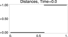
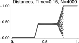
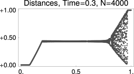
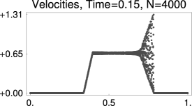
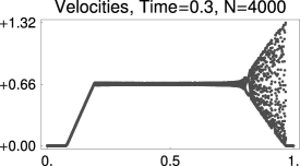
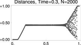
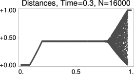
Figure 3.1: Numerical results for potential (3.1) and Riemann initial data (3.2): Snapshots of atomic distances and velocity against the macroscopic particle index $\overline{\alpha}$ for several macroscopic times and $N=4000$. On the macroscopic scale the solutions becomes self-similar: a left moving rarefaction wave and a right moving dispersive shock are separated by a cold intermediate state.

 

Figure 3.2: Atomic distances from Figure 3.2 for different values of $N$.

Figures 3.2 and 3.2 provide of course a merely qualitative confirmation of our interpretation of the numerical data. A refined quantitative measurement with different $N$ would be possible but requires much more numerical effort for the following two reasons.

$(1)$ Since information propagates with infinite speed in the lattice system (2.1) cold states manifest only in the limit $N\to\infty$. For finite $N$ we find small fluctuations everywhere due to the discreteness of $\alpha$. Heuristically, we expect the amplitude of the fluctuations to decay exponentially with $N$ outside the space-time cone spanned by the fastest macroscopic speeds, but only algebraically with $N$ inside this cone. This expectation is supported by rigorous results for the Toda chain and the harmonic chain, see [Kam93, MP09], and implies that the cold intermediate state has superimposed fluctuations with amplitude $1/\sqrt{N}$. An accurate measurement of intermediate states and wave speeds inside the above cone therefore requires simulations with very large $N$.

$(2)$ Due to the oscillatory nature it is notoriously difficult to compare quantitatively the dispersive shocks for different values of $N$ or $\overline{t}$: Accurate values for the evolution of the envelopes are very hard to measure numerically, and the precise values of averaged quantities such as local mean values or numerical distribution functions depend for finite $N$ on the details of the implemented averaging algorithm.

In this paper we focus on the qualitative properties of FPU Riemann solutions. We aim to understand the macroscopic selection and composition rules for elementary waves and how turning points of $\Phi$ effect the qualitative structure of Riemann solutions. In particular, we do not intend to measure numerical convergence rates or to predict the wave parameters quantitatively.

3.2 Elementary waves

The following key observation about solutions to FPU-Riemann problems reflects the hyperbolic and modulation nature of the limit $\varepsilon\to 0$, but has not yet been proven rigorously.

Observation 3.1.

For strictly monotone and nonlinear flux $\Phi^{\prime}$ where $\Phi^{\prime\prime\prime}$ has at most one root in the range of the solution we observe the following.

• The macroscopic dynamics for cold Riemann data is self-similar and hence reducible to the macroscopic velocity variable $c={\left({{\overline{\alpha}}-{\overline{\alpha}}_{*}}\right)}/{\overline{t}}$.

• The arising measure at each $({\overline{\alpha}},{\overline{t}})$ is either a point measure or supported on a closed curve that is generated by the distances and velocities of a wave train profile. Therefore, we can describe the macroscopic limit by a family of modulated wave trains parameterized by $c$.

• The macroscopic solution to each cold Riemann problem consist of a finite number of self-similar waves. These elementary waves are

  1. cold rarefaction waves,

  2. dispersive shock fans connecting two cold states,

  3. energy conserving jumps between two cold states (only for flux with turning point),

  4. dispersive shock fans connecting a cold state and a constant wave train; these shocks always come as a counter-propagating pair.

Structure of dispersive shocks

Our basic numerical observations concerning dispersive shocks are as follows, see also Figure 1.3. As mentioned in §1, dispersive shocks have been studied for certain potentials and in other contexts, but we have not found the following explicitly mentioned for FPU.

Observation 3.2.

In the numerical simulation of cold Riemann problems dispersive shocks appear with oscillatory atomic data between two constant states, see Figure 1.3. Within a dispersive shock the self-similarity variable $c={\left({\overline{\alpha}-\overline{\alpha}_{*}}\right)}/\overline{t}$ ranges between the shock back velocity $c_{\mathrm{b}}$ and the shock front velocity $c_{\mathrm{f}}$. The atomic oscillations have monotone envelopes with maximal amplitude at the front and vanishing at the back. There exist dispersive $1$-shocks with $c_{\mathrm{f}}<0$ and $c_{\mathrm{f}}<c_{\mathrm{b}}$ as well as dispersive $2$-shocks with $c_{\mathrm{f}}>0$ and $c_{\mathrm{f}}>c_{\mathrm{b}}$.

Moreover, our numerical results suggest the following fine-structure of the oscillations within a dispersive shock.

Observation 3.3.

A dispersive shock consists of a one-parameter family of wave trains parameterised by $c={\left({\overline{\alpha}-\overline{\alpha}_{*}}\right)}/\overline{t}$. Within the dispersive shock the parameter modulation is smooth (and hence follows a rarefaction wave of Whitham’s modulation equations). Dispersive $2$-shocks have the following properties (1-shocks accordingly due to symmetry).

• The measure $\mu{\left({c_{\mathrm{b}}}\right)}$ at the back of the shock reduces to the point measure generated by the constant left state $u_{{\mathrm{L}}}$, and the local mean values of atomic distances and velocities smoothly connect to $u_{{\mathrm{L}}}$.

• The measure $\mu{\left({c_{\mathrm{f}}}\right)}$ at the front of the shock converges to a soliton with background state $u_{{\mathrm{R}}}$, and the local mean values are continuous but not differentiable at $c_{\mathrm{f}}$.

• The family of curves $\mathrm{supp}(\mu(c))$ with $c_{\mathrm{b}}<c<c_{\mathrm{f}}$ is nested.

• The dispersive shock is compressive in the sense that both positive characteristic speeds $\lambda_{\pm}$ of the p-system point into the fan, i.e. $\lambda_{+}{\left({u_{{\mathrm{L}}}}\right)}>c_{\mathrm{b}}$ and $\lambda_{+}{\left({u_{{\mathrm{R}}}}\right)}<c_{\mathrm{f}}$.

• The Rankine-Hugeniot velocity of the jump lies strictly between $c_{\mathrm{b}}$ and $c_{\mathrm{f}}$.

For sufficiently small jump heights ${\left|{r_{\mathrm{R}}-r_{\mathrm{L}}}\right|}+{\left|{v_{\mathrm{R}}-v_{\mathrm{L}}}\right|}$ the shock back and front move in the same direction, this means we have either $c_{\mathrm{f}}<c_{\mathrm{b}}<0$ or $c_{\mathrm{f}}>c_{\mathrm{b}}>0$. The classical ‘piston problem’, however, shows that the situation is more subtle for large jump heights. The initial data in this problem describe an evenly spaced chain with positive left velocities and negative right velocities. It has been observed in [HS78] that sufficiently large (‘supercritical’) jumps in the velocity generate a transition from a pair of counter-propagating dispersive shocks with cold intermediate state to incomplete dispersive shocks whose ‘backs’ are constant binary oscillations which replace the cold intermediate state. This phenomenon is related to dispersive shock fans with counter-propagating back and front, see Figure 3.3(c). More precisely, passing the critical jump height from below the shock back velocities change their sign and the oscillatory intermediate state for supercritical data results from the interaction of two dispersive shocks. Analysing the back velocity of a dispersive shock might be a fruitful approach to determine the critical jump height in the piston problem.

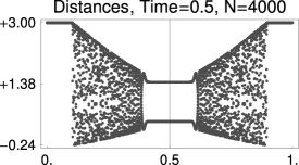
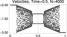
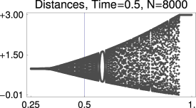
(a)	(b)	(c)

Figure 3.3: Snapshots for the Toda chain with initial jump at $\overline{\alpha}_{\ast}=0.5$ (see vertical lines). (a), (b) Distances and velocities for the classical ‘supercritical shock problem’ generating a permanent thermalization via binary oscillations; (c) Single dispersive shock where front and back counter-propagate; the asymptotic state at $\overline{\alpha}_{\ast}$ is a wave train with wave number $\sim 0.47$.

Conservative shocks in FPU chains

As discussed in §1, numerical simulations indicate that conservative shocks appear in FPU Riemann problems only if they are supersonic. For illustration we consider the two quintic potentials

$$\Phi(r+2) = r^{2}-\frac{r^{3}}{6}-\frac{r^{4}}{24}+\frac{r^{5}}{120}$$ (3.3)

$$\Phi(r+2) = r^{2}-\frac{r^{3}}{6}+\frac{r^{4}}{24}+\frac{r^{5}}{120}.$$ (3.4)

We plot the set of conservative shocks for these potentials in Figure 4.6. Note that due to Theorem 5.1(5) each of these sets consists of the diagonal and a closed curve crossing the diagonal at the turning points.

The flux $\Phi^{\prime}$ for (3.3) has a turning point $r_{*}\approx 1.3$ with $\Phi^{(4)}(r_{*})<0$ (convex-concave), while the flux for (3.4) has a turning point $r_{*}\approx 2.7$ with $\Phi^{(4)}(r_{*})>0$ (concave-convex). Both potentials are convex in a neighborhood of $r^{*}$, and the other turning points are outside the range of simulation.

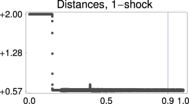
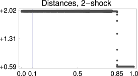
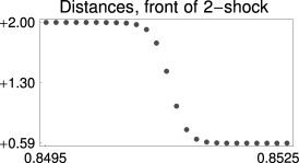
Figure 3.4: Supersonic conservative $1$- and $2$-shock for potential (3.3) with $N=8000$, $\overline{t}=0.5$ and ${\overline{\alpha}}_{\ast}$ indicated by the vertical lines.

Potential (3.3) allows for instance for the two supersonic conservative shocks

$$r_{\mathrm{L}}=2,\quad r_{\mathrm{R}}\approx 0.59,\quad c_{\mathrm{rh}}=\pm 1.50,\quad v_{\mathrm{R}}-v_{\mathrm{L}}\approx\pm 2.11,\quad\lambda_{\pm}(r_{\mathrm{L}})\approx\pm 1.41,\quad\lambda_{\pm}(r_{\mathrm{R}})\approx\pm 0.89.$$

In Figure 3.4 we plot the solution to the corresponding FPU-Riemann problem (with $v_{\mathrm{L}}=0$) and conclude that both the supersonic $1$-shock and the supersonic $2$-shock are captured by the atomic chain.

The conservative shocks for potential (3.4) that range over $r_{*}=2.7$, however, are subsonic. The FPU solution to

$$r_{\mathrm{L}}=4,\quad{}r_{\mathrm{R}}\approx 1.24,\quad c_{\mathrm{rh}}\approx\pm 1.46,\quad v_{\mathrm{R}}-v_{\mathrm{L}}\approx\pm 4.03,\quad\lambda_{\pm}(r_{\mathrm{L}})\approx\pm 1.83,\quad\lambda_{\pm}(r_{\mathrm{R}})\approx\pm 1.73,$$ (3.5)

is plotted in Figure 1.4, and is far from a conservative shock. Recall that this is accordance with the non-bifurcation result for subsonic fronts in [Ioo00]. The solution in Figure 1.4 consists of a dispersive shock with attached rarefaction wave, that means both waves are not separated by a constant state. Consequently, the soliton at the front of the dispersive shock is no longer supersonic but sonic, i.e., its speed equals the sound speed of the background state. This is confirmed by the numerical data in Figure 1.4(c): the distribution function near the soliton has the predicted cusp shape. Compare with the non-degenerate exponentially decaying soliton in Figure 1.3(c).

4 Riemann solvers

4.1 Towards an FPU-Riemann solver for the classical case

In this section we describe an adaption of the classical p-system solver that accounts for dispersive shocks in the macroscopic solutions to FPU-Riemann problems. Based on Observations 3.2 and 3.3 we arrive at the following conjecture, which is illustrated Figure 4.1.

Conjecture 4.1.

From each state $u_{{\mathrm{L}}}$ there emanate two dispersive shock curves $\mathcal{D}_{-}[u_{{\mathrm{L}}}]$ and $\mathcal{D}_{+}[u_{{\mathrm{L}}}]$ with the following properties.

• Each state $u_{{\mathrm{R}}}\in\mathcal{D}_{\pm}[u_{{\mathrm{L}}}]$ can be connected with $u_{{\mathrm{L}}}$ by a single dispersive shock with $\mathrm{sgn}(c_{\mathrm{f}})=\pm 1$.

• The curves fit smoothly to the corresponding rarefaction curves $\mathcal{R}_{\pm}[u_{{\mathrm{L}}}]$ (so that for small jump heights the dispersive and Lax-shock curves almost coincide).

The macroscopic solution to FPU-Riemann problems with cold data and sufficiently small jump heights can be described by the wave sets

$$\mathcal{W}^{\rm\,FPU}_{\pm}[u_{{\mathrm{L}}}]=\mathcal{R}_{\pm}[u_{{\mathrm{L}}}]\cup\mathcal{D}_{\pm}[u_{{\mathrm{L}}}].$$

In particular, a FPU-Riemann solution consists of a unique $1$-wave from $\mathcal{W}^{\rm\,FPU}_{-}[u_{{\mathrm{L}}}]$, an intermediate state $u_{{\mathrm{M}}}$, and a unique $2$-wave $\mathcal{W}^{\rm\,FPU}_{+}[u_{{\mathrm{M}}}]$. The intermediate state is cold if either a rarefaction wave occurs or if adjacent shock backs move away from each other; otherwise it is a wave train.

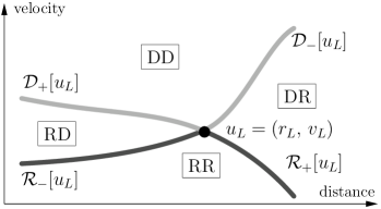
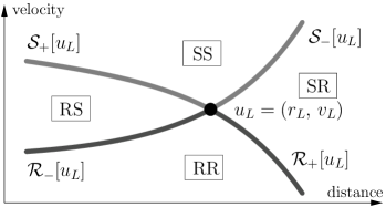
Figure 4.1: Left: Sketch of the FPU Riemann-solver for strictly convex $\Phi^{\prime}$. The wave sets $\mathcal{W}^{\rm\,FPU}[u_{\mathrm{L}}]$ consist of rarefaction curves and dispersive shock curves, and decompose the plane into 4 regions DD, RD, RR, and RD. Right: The corresponding classical solver for the p-system with Lax shocks instead of dispersive shocks.

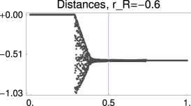
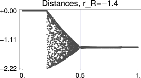
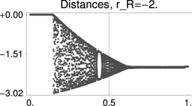
Figure 4.2: Three points from the dispersive shock curve $\mathcal{D}_{-}[{\left({0},\,{0}\right)}]$ for potential (3.1).

To illustrate the first part of this conjecture we present simulations for the modified Toda potential (3.1). For given left state $u_{{\mathrm{L}}}={\left({0},\,{0}\right)}$ and different values of $r_{\mathrm{R}}<0$ we choose $v_{\mathrm{R}}$ such that $u_{{\mathrm{R}}}={\left({r_{\mathrm{R}}},\,{v_{\mathrm{R}}}\right)}\in{}\mathcal{S}_{-}[u_{{\mathrm{L}}}]$, and study the macroscopic behaviour for the corresponding solutions to Newton’s equations. The results for ${\overline{\alpha}}_{*}=0.5$, $\overline{t}=0.1$, and $N=4000$ are depicted in Figure 4.2. For all values of $r_{\mathrm{R}}$ we find a dispersive $1$-shock whose front moves to the left, and an essentially cold intermediate state $u_{{\mathrm{M}}}$ which gives a point in $\mathcal{D}_{-}[u_{{\mathrm{L}}}]$. In all simulations there exists a right moving $2$-wave, but this wave has much smaller amplitudes than the $1$-wave. Hence, $\mathcal{D}_{-}[u_{{\mathrm{L}}}]$ and $\mathcal{S}_{-}[u_{{\mathrm{L}}}]$ are different but close to each other. Moreover, the simulations indicate the following behaviour for increasing jump height $r_{{\mathrm{L}}}-r_{\mathrm{R}}$. The shock front velocity $c_{\mathrm{f}}$ decreases, whereas $c_{\mathrm{b}}$ increases and changes its sign at a critical value of $r_{\mathrm{R}}$. As mentioned, this critical value can be viewed as the analogue to the critical parameter in the piston problem, see Figure 3.3.

Figure 4.3: Illustration of the FPU-Riemann solver for potential (3.1) and initial data (4.2). The examples IVP1–3 correspond to the regions RR, DR, and DD, respectively, in Figure 4.1.

The resulting FPU-Riemann solver is illustrated in Figure 4.3, which shows the solutions to the following initial value problems with $u_{\mathrm{L}}={\left({0},\,{0}\right)}$ and

$$\begin{array}[]{lclclclclcl}1:&u_{\mathrm{R}}={\left({0},\,{+1}\right)},&&2:&u_{\mathrm{R}}={\left({-1},\,{0}\right)},&&3:&u_{\mathrm{R}}={\left({0},\,{-1}\right)}.\end{array}$$ (4.2)

It is important to note that the Lax shock wave sets $\mathcal{S}_{\pm}[u_{{\mathrm{L}}}]$ generally differ from the dispersive shock wave sets $\mathcal{D}_{\pm}[u_{{\mathrm{L}}}]$. Therefore, replacing $\mathcal{S}_{\pm}[u_{{\mathrm{L}}}]$ by $\mathcal{D}_{\pm}[u_{{\mathrm{L}}}]$ changes the Riemann solution, i.e., the precise values for the intermediate state and possibly the waves themselves.

The difference between FPU chain and p-system can be quantified for the Toda potential (2.2). For the shock piston with $u_{{\mathrm{L}}}={\left({1},\,{+2a}\right)}$, $u_{{\mathrm{R}}}={\left({1},\,{-2a}\right)}$, and $0<a<1$ (subcritical case) the classical solver for the p-system provides the intermediate state $u_{{\mathrm{M}}}={\left({r_{M}},\,{0}\right)}$ with

$$4a^{2}={\left({r_{M}-1}\right)}{\Big{(}1-\exp{\left({1-r_{M}}\right)}\Big{)}}={\left({r_{M}-1}\right)}^{2}+\mathcal{O}{\big{(}{\left({r_{M}-1}\right)}^{3}\big{)}}$$

whereas the results in [Kam93] imply

$$r_{M}-1=2\ln{\left({a+1}\right)}{\left({a+1}\right)}^{2}=2a+\mathcal{O}{\big{(}a^{2}\big{)}}$$

for the FPU-Riemann solver. Both results are different but agree to leading order in $a$.

4.2 Riemann solvers for the p-system in the non-classical cases

In this section we consider forces $\Phi^{\prime}$ with a single turning point or where the solution ranges over at most one turning point. For the p-system, the classical Riemann solver cannot be used and also the above FPU-Riemann solver fails. To prepare the discussion of FPU-Riemann solvers in these cases, we first describe the relevant solvers of the p-system.

The building blocks for each non-classical solver are modified wave sets which replace $\mathcal{W}[u_{\mathrm{L}}]$ from the classical solver. Specifically, wave curves need to be adapted when intersecting the line $r=r_{\ast}$, though these start out near $u_{\mathrm{R}}=u_{\mathrm{L}}$ as classical wave sets (rarefaction waves and Lax shocks). The reason is the change in the sign of $\Phi^{\prime\prime\prime}$ at $r_{*}$, which implies that the Lax condition (A.2) or the compatibility condition $\lambda{\left({r_{\mathrm{R}}}\right)}>\lambda{\left({r_{\mathrm{L}}}\right)}$ is violated. Note that the wave curves directed away from the turning point $r_{\ast}$ remain unchanged. For a single turning point of the flux the classical wave sets interact with the turning point as follows.

Remark 4.2.

Let $u_{\mathrm{L}}$ with $r_{\mathrm{L}}\neq{r_{\ast}}$ be given and suppose convex-concave $\Phi^{\prime}$ with $\Phi^{(4)}{\left({r_{\ast}}\right)}<0$. Then the curves $\mathcal{R}_{+}[u_{\mathrm{L}}]$ and $\mathcal{S}_{-}[u_{\mathrm{L}}]$ intersect the line $r=r_{\ast}$ in the $(r,v)$-plane, whereas $\Phi^{\prime\prime\prime}$ does not change its sign along $\mathcal{R}_{-}[u_{\mathrm{L}}]$ and $\mathcal{S}_{+}[u_{\mathrm{L}}]$. The same holds for concave-convex $\Phi^{\prime}$ with $\Phi^{(4)}{\left({r_{\ast}}\right)}>0$ if we replace + by $-$.

• Proof. We start with convex-concave $\Phi$. For $r_{\mathrm{L}}<r_{\ast}$ we have $\Phi^{\prime\prime\prime}{\left({r_{\mathrm{L}}}\right)}>0$ and the formulas of Appendix A imply that both $\mathcal{R}_{+}[u_{\mathrm{L}}]$, $\mathcal{S}_{-}[u_{\mathrm{L}}]$ point into direction of increasing $r$, whereas $r$ decreases along $\mathcal{R}_{-}[u_{\mathrm{L}}]$ and $\mathcal{S}_{+}[u_{\mathrm{L}}]$; compare Figure 4.1 for an illustration of the wave sets of $u_{\mathrm{L}}$. The same is true for $r_{\mathrm{L}}>r_{\ast}$ as $\Phi^{\prime\prime\prime}{\left({r_{\mathrm{L}}}\right)}<0$ implies that now $r$ decreases along $\mathcal{R}_{+}[u_{\mathrm{L}}]$, $\mathcal{S}_{-}[u_{\mathrm{L}}]$. Finally, the proof for concave-convex $\Phi^{\prime}$ is analogous.  

The conservative solver

(a)	(b)

Figure 4.4: Modified wave sets of the conservative p-system solver: (a) modified shock curve, (b) modified rarefaction curve; C$=$compressive Lax shock, N$=$non-classical conservative shock, R$=$rarefaction wave; $\widetilde{\Phi}^{\prime}(r)$ as in the main text. In the insets we sketch an example for the different composite waves in each segment of the $r_{\mathrm{R}}$-axis.

The modified shock curve $\mathcal{S}_{-}^{\rm\,cons}[u_{\mathrm{L}}]$ of the conservative p-system solver is illustrated in Figure 4.4(a) for convex-concave $\Phi^{\prime}$ and $r_{\mathrm{L}}>r_{\ast}$. This is done by parameterizing $\mathcal{S}_{-}^{\rm\,cons}[u_{\mathrm{L}}]$ by $r_{\mathrm{R}}$ and plotting $\widetilde{\Phi}^{\prime}(r)=\Phi^{\prime}(r)+\rho_{1}r+\rho_{2}$ to give an illustrative graph. In accordance with Remark 4.2 the curve $\mathcal{S}_{-}^{\rm\,cons}[u_{\mathrm{L}}]$ starts out as $\mathcal{S}_{-}[u_{\mathrm{L}}]$ for $r_{\mathrm{R}}\lessapprox{}r_{\mathrm{L}}$. The wave set modification for large $r_{\mathrm{L}}-r_{\mathrm{R}}$ goes via conservative shocks and works as follows. Along $\mathcal{S}^{\rm\,cons}_{-}[u_{\mathrm{L}}]$ there exist a unique state $u_{0}={\left({r_{0}},\,{v_{0}}\right)}\in\mathcal{H}_{-}[u_{\mathrm{L}}]$ that can be reached from $u_{\mathrm{L}}$ with a single conservative $1$-shock. This state $u_{0}$ determines another state $u_{2}={\left({r_{2}},\,{v_{2}}\right)}$ corresponding to a Lax shock in $\mathcal{S}_{-}[u_{\mathrm{L}}]$ such that at $r_{2}$ the secant slope from $r_{\mathrm{L}}$ to $r_{2}$ coincides with the slope of the secant from $r_{\mathrm{L}}$ to $r_{0}$. This reads

$$r_{0}<r_{2}<r_{\mathrm{L}}\quad\text{and}\quad\frac{\Phi^{\prime}{\left({r_{\mathrm{L}}}\right)}-\Phi^{\prime}{\left({r_{2}}\right)}}{r_{\mathrm{L}}-r_{2}}=\frac{\Phi^{\prime}{\left({r_{0}}\right)}-\Phi^{\prime}{\left({r_{2}}\right)}}{r_{0}-r_{2}},$$

and implies that the Lax shock connecting $u_{\mathrm{L}}$ to $u_{2}$ and the conservative shock connecting $u_{\mathrm{L}}$ to $u_{0}$ have the same Rankine-Hugeniot velocity. Note that this relation and in fact all conservative shock distance data are the same for $\Phi^{\prime}$ and $\widetilde{\Phi}^{\prime}$.

The modified rarefaction curve $\mathcal{R}_{+}^{\rm\,cons}[r_{\mathrm{L}}]$ is illustrated in Figure 4.4(b) in the same way. The following lemma, which follows directly from results in [Smo94, LeF02], precisely describes the modified shock and rarefaction curves (for both convex-concave and concave-convex $\Phi^{\prime})$.

Lemma 4.3.

• If $\Phi^{\prime\prime\prime}(r)\neq 0$ for all $r\in I_{0}:=(r_{\mathrm{R}},r_{\mathrm{L}})$, then the solution coincides with the classical solution and consists of at most two uniquely chosen rarefaction fans or compressive shocks.

• Suppose $\Phi^{\prime\prime\prime}(r_{*})=0$ for a unique $r_{*}$ and let $u_{\mathrm{L}}=(r_{\mathrm{L}},v_{\mathrm{L}})$ with $r_{\mathrm{L}}>r_{*}$ be given. Then the following are uniquely defined for $r_{\mathrm{R}}<r_{\mathrm{L}}$. The solution $r_{0}$ of $\mathcal{J}(r_{\mathrm{L}},r_{0})=0$, the solution $r_{m}$ of $\mathcal{J}(r_{\mathrm{R}},r_{m})=0$, and the solutions $r_{1}$ of $|c_{\mathrm{rh}}(r_{\mathrm{L}},r_{1})|=|c_{\mathrm{rh}}(r_{\mathrm{L}},r_{m})|$ and $r_{2}$ of $|c_{\mathrm{rh}}(r_{\mathrm{L}},r_{2})|=|c_{\mathrm{rh}}(r_{\mathrm{L}},r_{0})|$. It holds that $r_{1}<r_{0}<r_{2}<r_{*}<r_{\mathrm{L}}$. Note that $r_{0},r_{2}$ depend only on $r_{\mathrm{L}}$ whereas $r_{m},r_{1}$ are functions of $r_{\mathrm{R}}$.

  1. Let $v_{0}$ be such that $u_{0}:=(r_{0},v_{0})\in\mathcal{H}_{\pm}[u_{\mathrm{L}}]$. A right state $u_{\mathrm{R}}$ with $r_{\mathrm{R}}<r_{\mathrm{L}}$ lies in the modified shock wave set $\mathcal{S}^{\rm\,cons}_{\pm}[u_{\mathrm{L}}]$ if $u_{\mathrm{R}}\in\mathcal{S}_{\pm}[u_{\mathrm{L}}]$ for $r_{2}<r_{\mathrm{R}}$, $u_{\mathrm{R}}\in\mathcal{S}_{\pm}[u_{0}]$ for $r_{0}<r_{\mathrm{R}}<r_{2}$, and $u_{\mathrm{R}}\in\mathcal{R}_{\pm}[u_{0}]$ for $r_{\mathrm{R}}<r_{0}$. By definition of $r_{0}$, the shock from $u_{\mathrm{L}}$ to $u_{0}$ is conservative, and the solution amplitude is discontinuous at $r_{2}$. There always is an intermediate state between rarefaction fan or compressive shock and conservative shock.

  2. Let $v_{m}$ be such that $u_{m}:=(r_{m},v_{m})\in\mathcal{H}_{\pm}[u_{\mathrm{R}}]$. A right state $u_{\mathrm{R}}$ with $r_{\mathrm{R}}<r_{\mathrm{L}}$ lies in the modified rarefaction wave set $\mathcal{R}^{\rm\,cons}_{\pm}[u_{\mathrm{L}}]$ if $u_{\mathrm{R}}\in\mathcal{R}_{\pm}[u_{\mathrm{L}}]$ for $r_{\mathrm{R}}>r_{*}$, $u_{m}\in\mathcal{R}_{\pm}[u_{\mathrm{L}}]$ for $r_{0}<r_{\mathrm{R}}<r_{*}$, $u_{m}\in\mathcal{S}_{\pm}[u_{\mathrm{L}}]$ for $r_{1}<r_{\mathrm{R}}<r_{0}$, and $u_{\mathrm{R}}\in\mathcal{H}_{\mp}[u_{\mathrm{L}}]$ for $r_{\mathrm{R}}<r_{1}$.

     By definition of $r_{m}$, for $r_{1}<r_{\mathrm{R}}<r_{*}$ the shock from $u_{m}$ to $u_{\mathrm{R}}$ is conservative, and the solution amplitude is discontinuous at $r_{1}$. For $r_{0}<r_{\mathrm{R}}<r_{*}$ the rarefaction fan is attached to the conservative shock, while for $r_{1}<r_{\mathrm{R}}<r_{0}$ the compressive shock is not.

• If the flux $\Phi^{\prime}$ has several turning points, then the modified wave sets are unchanged as long as $u_{\mathrm{L}}$, $u_{\mathrm{R}}$ are such that only one turning point lies in $[r_{1},r_{m}]$ and $[r_{0},r_{\mathrm{L}}]$.

• Proof. $(1.)$ Lemma 5.3(2.) shows that $\mathcal{J}\neq 0$ in this case. Hence, the conservative Riemann solver coincides with the classical solver [LeF02]. For this solver, the p-system is solved uniquely in terms of at most two rarefaction or shock waves [Smo94]. $(2.)$ The proof for the shock case is an immediate consequence of Theorem IV.4.3 (see also Theorem II.4.3) of [LeF02]. The rarefaction case is not explicitly proven in [LeF02], but follows from the exposition, cf. [LeF02] p.163 (see also Theorem II.5.4). $(3.)$ This follows from the independence of the solution on $\Phi$ outside this range.  

Due to this construction, the Riemann solution generically contains conservative shocks despite the fact that these are of higher codimension in the space of left and right states: A solution will consist of three elementary waves instead of two whenever a conservative shock is possible. Also note that the solution is non-monotone whenever a compressive and a conservative shock are connected in a solution.

The dissipative solver

We refer to the ‘maximum entropy dissipation’ solver in [LeF02] as the dissipative solver. This solver is much simpler than the conservative solver, and we do not explain it in as much detail. We plot the modified wave sets which determine the solver in Figure 4.5 for concave-convex $\Phi^{\prime}$ and $r_{\mathrm{L}}>r_{*}$. Compared with the conservative solver, the regions with conservative shocks have shrunk to points. The distance values where wave sets need to be modified are the turning point $r_{*}$ and the value $r_{0}^{*}$ where the compressive shock has extremal velocity, i.e., where it coincides with a characteristic velocity.

(a)	(b)

Figure 4.5: Modified wave sets of the dissipative p-system solver: (a) modified shock curve, (b) modified rarefaction curve; symbols as in Figure 4.4.

4.3 Towards an FPU-Riemann solver for the non-classical supersonic case

We numerically tested the predictions of the conservative solver about the modified wave sets by simulations with initial data on the p-system shock and rarefaction curves. From the classical case we expect that compressive shocks are replaced by dispersive shocks in the FPU chain. Indeed, up to this modification, for convex-concave potentials the conservative solver qualitatively makes the correct predictions for FPU chains.

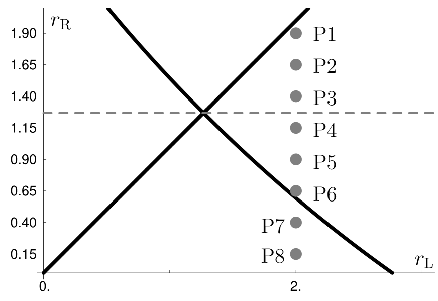
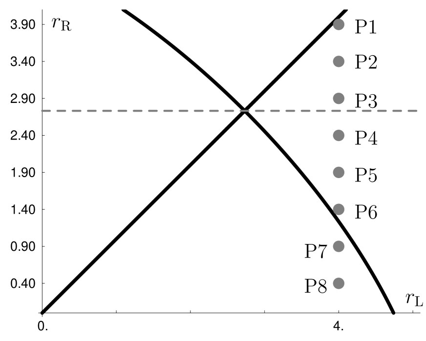
(a)	(b)

Figure 4.6: Part of conservative shock data for the potentials (3.3) in (a) and (3.4) in (b). The horizontal lines mark the turning point. Bullets mark the locations of $(r_{\mathrm{L}},r_{\mathrm{R}})$ for the simulations the simulations plotted in Figures 4.8 and 4.8 for (a), as well as Figures 4.10 and 4.10 for (b).

Figure 4.7: Simulations for data on the supersonic $1$-shock curve for potential (3.3) and $u_{\mathrm{L}}=(2,0)$, $\overline{\alpha}_{\ast}=0.9$, $\overline{t}=0.5$, $N=2000$. The values for $r_{\mathrm{R}}$ are those in Figure 4.6(a), so ‘IVP Sx’ crosses the turning point for increasing $x$.

Figure 4.8: Simulations for data on the $2$-rarefaction curve for potential (3.3) analogous to Figure 4.8.

In order to illustrate the structure of the modified wave sets for (3.3) we proceed as follows. We fix the left state $u_{\mathrm{L}}={\left({2},\,{0}\right)}$, and for the points $Px$ marked in Figure 4.6(a) we solve two Riemann problems denoted by $Sx$ and $Rx$. The value for ${r_{\mathrm{R}}}$ is determined by $Px$, whereas ${v_{\mathrm{R}}}$ is chosen such that, for the p-system, $Sx$ and $Rx$ correspond to a single $1$-shock and $2$-rarefaction wave, respectively. The numerical results for the atomic chain are plotted in Figures 4.8 and 4.8.

Neglecting small waves and fluctuations (caused by the computational boundary and the positivity of ${\varepsilon}$) the simulations provide numerical evidence that the macroscopic limit can indeed be described by a modified conservative solver. The solutions for $S1$ to $S8$ correspond to those in Figure 4.4(a) when replacing compressive by dispersive shocks, and we use the inset titles C, N+C, N+R in the following. For small jump, i.e. $r_{\mathrm{R}}\lessapprox{}r_{\mathrm{L}}$, the chain produces dispersive $1$-shocks with amplitudes proportional to the jump height ($S2,S3\cong$ C), and there exists a critical point $r_{\mathrm{R}}=\hat{r}_{2}$ at which the unique supersonic conservative shock nucleates. For $r_{\mathrm{R}}<\hat{r}_{2}$ the conservative shock persists whereas the dispersive shock shrinks ($S4,S5,S6\cong$ N+C) and transforms into a rarefaction wave ($S7\cong$ N+R). Note that, in contrast to the conservative p-system solver, the nucleation of the conservative shock is a continuous transition in the envelope since the dispersive shock extends to the nucleating intermediate state. In the same way the solutions of $R1$ to $R8$ transform to those of Figure 4.4(b), again using inset titles: $R1,R3\cong$ R, $R5,R6\cong$ R+N (with $R6$ near N only), $R7,R8\cong$ C+N.

We summarize these modifications for the non-classical supersonic case in the following conjecture.

Conjecture 4.4.

For convex-concave flux Lemma 4.3 holds under the following modifications and thereby defines the modified shock wave sets $\mathcal{S}_{\pm}^{\mathrm{FPU}}[u_{\mathrm{L}}]$ and the modified rarefaction wave sets $\mathcal{R}_{\pm}^{\mathrm{FPU}}[u_{\mathrm{L}}]$ for the macroscopic FPU chain: (1) Replace Lax-shocks by dispersive shocks in the definition of $\mathcal{S}_{\pm}^{\rm\,cons}[u_{\mathrm{L}}]$, i.e., use $\mathcal{D}_{\pm}[u_{\mathrm{L}}]$ from §4.1. (2) Replace $r_{2}$ by the solution $\hat{r}_{2}$ of $|c_{\mathrm{f}}(r_{\mathrm{L}},\hat{r}_{2})|=|c_{\mathrm{rh}}(r_{\mathrm{L}},r_{0})|$, and $r_{1}$ by the solution $\hat{r}_{1}$ of $|c_{\mathrm{f}}(r_{m},r_{\mathrm{L}})|=|c_{\mathrm{rh}}(\hat{r}_{1},r_{m})|$.

4.4 Towards an FPU-Riemann solver for the non-classical subsonic case

For subsonic conservative shock data, the situation is entirely different. Recall that in Figure 1.4 subsonic conservative shock initial data did not produce a conservative shock. From §2 recall that fronts of the infinite chain do not bifurcate in the subsonic case. Indeed, simulations analogous to those in the supersonic case yield the drastically different results plotted in Figures 4.10 and 4.10. Since conservative shocks are absent and composite wave of rarefaction and dispersive shocks occur, we compare these with the solutions of the dissipative p-system solver. It is the only solver in the (natural) family of solvers studied in [LeF02] that does not use non-classical shocks, compare Figure 4.5.

We investigate the modified wave sets for potential (3.4) as before. For given left state $u_{\mathrm{L}}={\left({4},\,{0}\right)}$ we choose several values of $r_{\mathrm{R}}$, see Figure 4.6, and determine $v_{\mathrm{R}}$ such that $u_{\mathrm{R}}={\left({r_{\mathrm{R}}},\,{v_{\mathrm{R}}}\right)}$ belongs to $\mathcal{R}_{-}[u_{\mathrm{L}}]$ and $\mathcal{S}_{+}[u_{\mathrm{L}}]$. The numerical results are plotted in Figures 4.10 and 4.10; for comparison with the dissipative p-system solver we use the inset titles from Figure 4.5. For the shock initial data $S1$–$S5$ the chain produces single dispersive shocks ($S1$–$S5\cong$ C) with increasing amplitudes, decreasing back speeds $c_{\mathrm{b}}$ and increasing front speeds $c_{\mathrm{f}}$. Here $c_{\mathrm{f}}$ is always larger than the corresponding Rankine-Hugeniot speed $c_{\mathrm{rh}}$ and the speed of the conservative shock. For $S6$–$S8\cong$ C+R we find a qualitatively different solution with increasing rarefaction waves that are attached to the same dispersive shock.

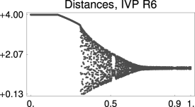
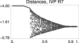
Figure 4.9: Simulations for data on the $2$-shock curve for potential (3.4) and $u_{\mathrm{L}}=(4,0)$, and $\overline{\alpha}_{\ast}=0.1$, $N=3000$, $\overline{t}=0.4$. The values for $r_{\mathrm{R}}$ are those in Figure 4.6(b), so ‘IVP $Sx$’ crosses the turning point for increasing $x$. The vertical lines indicate the locations of the $2$-shocks of the p-system corresponding to ${\left({r_{\mathrm{L}}},\,{r_{\mathrm{R}}}\right)}$, and the conservative shock corresponding to $u_{\mathrm{L}}$.

Figure 4.10: Simulations for data on the $1$-rarefaction curve for potential (3.4) analogous to Figure 4.10.

On the other hand, in the sequence $R1$–$R8$ the solutions are single rarefaction waves ($R2\cong$ R), from which a dispersive shock nucleates between $R3$ and $R4\cong$ R+N, when crossing the turning point $r_{*}$, see Figure 4.6(b). The rarefaction fan shrinks from $R5$ to $R7$, and eventually the solution consists of a single dispersive shock (not shown) corresponding to inset C in Figure 4.5(b). We conjecture that the solutions from both Figures 4.10 and 4.10 can be understood by modifying the dissipative solver as explained below. However, since there are no non-classical shocks to test against, and since we cannot compute $c_{\mathrm{f}}$ from the left and right states, our evidence is weaker than in the supersonic case.

(a)	(b)

Figure 4.11: (a) Sketch of the explanation for non-nucleation in the subsonic case. Here the front velocity $c_{\mathrm{f}}$ is larger than the nucleation velocity so that conservative shocks cannot be selected. (b) In the supersonic case, the nucleation cannot be missed in this way and occurs here at $r_{2}^{*}$.

We numerically observed the absence of subsonic conservative shocks for various potentials. An explanation on the level of the Riemann solver is the following. Along the conservative shock-curve $\mathcal{S}_{+}^{\rm\,cons}[u_{\mathrm{L}}]$ of the p-system, the nucleation of the conservative shock connecting to $u_{\mathrm{L}}$ occurs when it is as slow as the compressive shock, i.e., $c_{\mathrm{rh}}(r_{\mathrm{L}},r_{0})=c_{\mathrm{rh}}(r_{\mathrm{L}},r_{\mathrm{R}})$. However, in the FPU case, the criterion is naturally modified to equality of conservative shock velocity and front velocity of the dispersive shock, i.e., $c_{\mathrm{rh}}(r_{\mathrm{L}},r_{0})=c_{\mathrm{f}}(r_{\mathrm{L}},r_{\mathrm{R}})$. Recall that we have $c_{\mathrm{f}}(r_{\mathrm{L}},r_{\mathrm{R}})>c_{\mathrm{rh}}(r_{\mathrm{L}},r_{\mathrm{R}})$ for $r_{\mathrm{R}}\neq r_{\mathrm{L}}$ due to Observation 3.2, and note that both velocities converge to the characteristic velocity as $r_{\mathrm{R}}\to r_{\mathrm{L}}$. It is therefore plausible that $c_{\mathrm{f}}(r_{\mathrm{L}},r_{\mathrm{R}})>c_{\mathrm{rh}}(r_{\mathrm{L}},r_{0})$ for all $r_{\mathrm{R}}$ so that the nucleation criterion always fails. We sketch this situation in Figure 4.11(a). Note that the relative locations of the $2$-shock and the dispersive shock front in Figure 4.10 support that this ordering indeed occurs for the potential (3.4).

In contrast, in the supersonic case $\Phi^{(4)}(r_{*})<0$ the velocity curve is unimodal with a maximum, so that nucleation cannot be missed in this way, see Figure 4.11(b). We thus arrive at the following conjecture.

Conjecture 4.5.

Let $r_{*}$ be the unique turning point of $\Phi^{\prime}$. If $\Phi^{(4)}(r_{*})<0$, then non-classical shocks are absent and the solution is qualitatively according to the dissipative solver. More precisely, the wave sets depicted in Figure 4.5 need to be modified as follows: (1) Replace Lax-shocks by dispersive shocks in the definition of $\mathcal{S}_{\pm}^{\rm\,cons}[u_{\mathrm{L}}]$, i.e., use $\mathcal{D}_{\pm}[u_{\mathrm{L}}]$ from §4.1. (2) Replace $r_{0}^{*}$ by the solution $\hat{r}_{0}^{*}$ to $c_{\mathrm{f}}(\hat{r}_{0}^{*},r_{\mathrm{L}})^{2}=\Phi^{\prime\prime}(\hat{r}_{0}^{*})$ and $r_{1}^{*}$ by the solution $\hat{r}_{1}^{*}$ to $c_{\mathrm{f}}(\hat{r}_{0}^{*},r_{\mathrm{L}})^{2}=\Phi^{\prime\prime}(r_{\mathrm{L}})$.

5 Properties of conservative shocks

In this section we study conservative shocks, that means solutions to the three independent jump conditions (2.7). Eliminating the velocities $v_{\mathrm{L}}$, $v_{\mathrm{R}}$, an $c_{\mathrm{rh}}$ one finds that each conservative shock is an element of

$$D=\left\{{\left({r_{\mathrm{L}}},\,{r_{\mathrm{R}}}\right)}\;:\;\mathcal{J}{\left({r_{\mathrm{L}}},\,{r_{\mathrm{R}}}\right)}=0\right\},$$ (5.1)

with $\mathcal{J}$ as in (2.8). Conversely, each point in $D$ defines both a conservative $1$-shock and a $2$-shock, which are unique up to Galilean transformation and differ only in $\mathrm{sgn}{|\![v]\!|}=\mathrm{sgn}\,{c_{\mathrm{rh}}}$. The geometric interpretation of $\mathcal{J}=0$ is that the signed area between the graphs of $\Phi^{\prime}$ and the secant line through $\Phi^{\prime}(r_{\mathrm{L}})$ and $\Phi^{\prime}(r_{\mathrm{R}})$ is zero over $[r_{\mathrm{L}},r_{\mathrm{R}}]$, compare Figure 5.1.

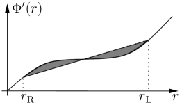
(a)	(b)	(c)

Figure 5.1: Sample sketches for $\mathcal{J}(r_{\mathrm{L}},r_{\mathrm{R}})=0$. Between $r_{\mathrm{L}}$ and $r_{\mathrm{R}}$ the areas above and below the secant line up to the graph of $\Phi^{\prime}$ (shaded) are equal. (a) The secant transversely intersects the graph on left and right so that the set $D$ is locally a monotone curve in the $(r_{\mathrm{L}},r_{\mathrm{R}})$-plane. (b) Secant and graph are tangent at $r_{\mathrm{L}}$ so that $D$ has a local extremum in the $(r_{\mathrm{L}},r_{\mathrm{R}})$-plane. $\Phi^{\prime}$ has (at least) two turning points in $[r_{\mathrm{R}},r_{\mathrm{L}}]$. (c) The secant is tangent at both intersection points, and both tangencies point in the same direction, hence it is a local extremum of $\mathcal{J}$ and the point $(r_{\mathrm{L}},r_{\mathrm{R}})$ is isolated in $D$. $\Phi^{\prime}$ has (at least) four turning points in $[r_{\mathrm{R}},r_{\mathrm{L}}]$

To characterise the structure of $D$ in presence of several turning points of $\Phi^{\prime}$ we use the notation $c_{\mathrm{L}}:=|\lambda_{\pm}(r_{\mathrm{L}})|$ and $c_{\mathrm{R}}:=|\lambda_{\pm}(r_{\mathrm{R}})|$.

Theorem 5.1.

For $\Phi\in C^{4}(\mathbb{R})$ the set $D$ has the following properties.

• Off-diagonal data $(r_{\mathrm{L}},r_{\mathrm{R}})\in D$ with $r_{\mathrm{L}}\neq r_{\mathrm{R}}$ exists if and only if $\Phi^{\prime}$ has at least one turning point in the interval $(r_{\mathrm{L}},r_{\mathrm{R}})$.

• Let $I\subset\mathbb{R}$ be any interval containing a single turning point of $\Phi^{\prime}$. Then $D\cap I\times{I}$ is the graph of a strictly decreasing function which crosses the diagonal $\{r_{\mathrm{L}}=r_{\mathrm{R}}\}$ at the turning point.

• The conservative shocks corresponding to $D\cap{I}\times{I}$ are undercompressive. If $\Phi^{(4)}(r_{*})<0$, they are supersonic, and if $\Phi^{(4)}(r_{*})>0$ subsonic.

• Compression changes precisely at local extrema in the coordinate directions of $D$ in the $(r_{\mathrm{L}},r_{\mathrm{R}})$-plane. At extrema in the $r_{\mathrm{L}}$-direction $c_{\mathrm{R}}^{2}$ crosses $c_{\mathrm{rh}}(r_{\mathrm{L}},r_{\mathrm{R}})^{2}$, and at extrema in the $r_{\mathrm{R}}$-direction $c_{\mathrm{L}}^{2}$ crosses $c_{\mathrm{rh}}(r_{\mathrm{L}},r_{\mathrm{R}})^{2}$.

• If $\Phi^{\prime}$ has precisely two turning points, then $D$ is the union of the diagonal $\{r_{\mathrm{L}}=r_{\mathrm{R}}\}$ and a closed curve crossing the diagonal at the turning points.

• The set $D$ does not have bounded connected components if $\Phi^{\prime}$ has three or fewer turning points, and $D\setminus\{r_{\mathrm{L}}=r_{\mathrm{R}}\}$ is bounded if the number of turning points is even.

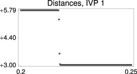
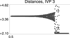
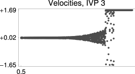
(a)	(b)	(c)

Figure 5.2: (a) The set $D$ for the potential (5.2), i.e., on solid curves holds $\mathcal{J}=0$; off-diagonal segments of $D$ are labelled according to the ordering of $c_{\mathrm{rh}}^{2}$ and $\lambda_{\pm}^{2}$. (b) Solution for a conservative shock with initial data at point (1) in (a). (c) Solution for the initial data from point (3) in (a); the solutions appears to contain a jump from wave train to wave train. In (b) & (c) the initial data ranges over two turning points of $\Phi^{\prime}$; $N=4000$ initial jump ${\overline{\alpha}}_{*}=0.5$.

In Figure 5.2(a) part of the set $D$ is plotted for the potential

$$\Phi(r+1)=r+\frac{1}{2}r^{2}+\frac{1}{20}r^{3}-\frac{1}{4}\cos(2r)+\frac{1}{10}\sin(3r).$$ (5.2)

Changes in shock type occur for instance at point 2, which is an extremum in the $r_{\mathrm{R}}$-direction so that $c_{\mathrm{L}}^{2}$ becomes larger than $c_{\mathrm{rh}}^{2}$ in the direction towards the nearest extremum in $r_{\mathrm{L}}$-direction at point 4. The conservative shocks on this curve start out supersonic, hence in the segment between points 2 and 4 the 1-shocks are compressive and the 2-shocks are rarefaction shocks. At point 4 the term $c_{\mathrm{R}}^{2}$ becomes larger than $c_{\mathrm{rh}}^{2}$ when crossing it away from point 3, and so conservative shocks beyond point 4 are subsonic.

Remark 5.2.

• Conservative shocks do not have a preferred direction of propagation, and are isolated points on the shock curves $\mathcal{S}_{\pm}[u_{\mathrm{L}}]$. In contrast, classical shocks have a selected direction of propagation in order to be compressive and generate continuous segments of $\mathcal{S}_{\pm}[u_{\mathrm{L}}]$.

• In lack of turning points, conservative shock data does not exist for the Toda potential and any cubic potential. For harmonic potentials, however, all shocks are conservative, and in fact contact discontinuities.

• For even potentials off-diagonal conservative jumps occur for $r_{\mathrm{L}}=-r_{\mathrm{R}}$, because $\mathcal{J}(r,-r)\equiv 0$ by symmetry. More generally, the symmetry $\Phi(r_{*}+r)=\Phi(r_{*}-r)$ with $\Phi^{\prime\prime\prime}(r_{*})=0$ provides $\tilde{D}\subset{D}$ with $\tilde{D}=\left\{(r_{\mathrm{L}},r_{\mathrm{R}})=(r_{*}+r,r_{*}-r):r\in\mathbb{R}\right\}.$ Note that each conservative shock from $\tilde{D}$ is degenerate as the characteristic velocities for left and right states equal.

• For quartic potentials (i.e., the classical FPU chains) all off-diagonal conservative data are given by $\tilde{D}$, so that non-degenerate conservative shocks occur only for potentials of polynomial degree five or higher.

• Proof of Theorem 5.1

  • This immediately follows from the geometric interpretation of $\mathcal{J}=0$, see Figure 5.1.

  • Again, the geometric interpretation shows that for fixed $r_{\mathrm{L}}\subset I$ there is at most one solution $r\in I$ to $\mathcal{J}(r_{\mathrm{L}},r)=0$; similar for $r_{\mathrm{R}}$. Hence, the solution set is a monotone curve; that it decays follows similarly. Note that tangents of $\Phi$ and the secant slope cannot coincide within $I$.

  • & 4. These follow from Lemma 5.3 below.

  • Consider $(r_{\mathrm{L}},r_{\mathrm{R}})$ as in Figure 5.1(b), where $\mathcal{J}(r_{\mathrm{L}},r_{\mathrm{R}})=0$ and the secant slope coincides with the tangent slope of $\Phi^{\prime}$ at one end. Note that, since there are only two turning points, the graph of $\Phi^{\prime}$ must lie on one side of the secant line near the tangency. Moving monotonically through the point where these slopes coincide, the area between the graphs can only vanish when the other point reverses its direction. Hence, the curve in the $(r_{\mathrm{L}},r_{\mathrm{R}})$-plane has an extremum, and this can only occur when both turning points lie in the interval $(r_{\mathrm{R}},r_{\mathrm{L}})$. When continuing the curves from item 2, the tangency points of the graph intersections must be reached. Since there are no further changes in monotonicity, and curves are unique in suitable intervals $I$, the two curves emanating from the turning points must connect.

    It remains to show that there can be no bounded components of $D$ that are isolated from the diagonal.

    Note that a stationary point ${\left({r_{\mathrm{L}}^{*}},\,{r_{\mathrm{R}}^{*}}\right)}$ of $\mathcal{J}$ requires tangency of the graph of $\Phi^{\prime}$ with the secant segment at both $r_{\mathrm{L}}^{*}$ and $r_{\mathrm{R}}^{*}$. Such a stationary point is a local extremum if the graph of $\Phi^{\prime}$ is either above or below the common tangency at both $r_{\mathrm{L}}^{*}$ and $r_{\mathrm{R}}^{*}$, i.e., $\Phi^{\prime\prime\prime}{\left({r_{\mathrm{L}}^{*}}\right)}$ and $\Phi^{\prime\prime\prime}{\left({r_{\mathrm{R}}^{*}}\right)}$ have the same sign. For $\Phi$ with two turning points there exist a unique stationary point which is moreover a local extremum $(r^{*}_{\mathrm{L}},r^{*}_{\mathrm{R}})$ with $\mathcal{J}(r^{*}_{\mathrm{L}},r^{*}_{\mathrm{R}})\neq 0$, because the geometry implies that the enclosed area is only on one side of the secant. Hence, each zero of $\mathcal{J}$ is a regular point and cannot be an isolated point of $D$. Now suppose for contradiction that a connected and bounded component of $D$ existed. Then it must be a closed curve containing the local extremum ${\left({r_{\mathrm{L}}^{*}},\,{r_{\mathrm{R}}^{*}}\right)}$ in its interior. However, fixing $r^{*}_{\mathrm{L}}$ and moving from $r^{*}_{\mathrm{R}}$ towards $r^{*}_{\mathrm{L}}$ the secant segment stays above or below the graph of $\Phi^{\prime}$ so that $\mathcal{J}\neq 0$ until $r_{\mathrm{L}}=r_{\mathrm{R}}$ on the diagonal, which is the contradiction.

  • We continue the discussion of bounded isolated components from the previous item with a local extremum ${\left({r_{\mathrm{L}}^{*}},\,{r_{\mathrm{R}}^{*}}\right)}$ in the interior. Our arguments from above imply that the interval $[r_{\mathrm{R}}^{*},r_{\mathrm{L}}^{*}]$ contains at least three turning points, and the tangency criterion for local extrema shows that the number of turning points in the interval must be even.

    Concerning boundedness of $D\setminus\{r_{\mathrm{L}}=r_{\mathrm{R}}\}$, note that for an even number of turning points, the convexity of $\Phi^{\prime}$ outside a sufficiently large interval is the same. Hence, the secant line for sufficiently far distant $r_{\mathrm{L}}$ and $r_{\mathrm{R}}$ lies on one side of the graph of $\Phi^{\prime}$ so that $\mathcal{J}\neq 0$.

   

Using the proof of the last item, it is not difficult to construct $\Phi$ for which the set $D$ consists of several bounded components that are disconnected from each other. The following lemma gives some more specific information.

Lemma 5.3.

• Whenever $\Phi^{\prime\prime\prime}(r_{*})=0$ and $\Phi^{(4)}(r_{*})\neq 0$ for some $r_{*}\in\mathbb{R}$ there exist a smooth locally unique curve $r_{\mathrm{L}}\mapsto{R}{\left({r_{\mathrm{L}}}\right)}$ of solutions to $\mathcal{J}=0$ in $\{r_{\mathrm{L}}\neq r_{\mathrm{R}}\}\cup\{(r_{*},r_{*})\}$ and it has tangent $(-1,1)$ at $(r_{*},r_{*})$.

• Whenever $c_{\mathrm{rh}}^{2}(r_{\mathrm{L}},r_{\mathrm{R}})\neq c_{\mathrm{R}}^{2}$ and $\mathcal{J}(r_{\mathrm{L}},r_{\mathrm{R}})=0$ then the set $D$ from Theorem 5.1 is locally given by a function $r_{\mathrm{R}}=R(r_{\mathrm{L}})$, which has a local extremum if $c_{\mathrm{rh}}^{2}(r_{\mathrm{L}},r_{\mathrm{R}})=c_{\mathrm{L}}^{2}$. Similarly, whenever $c_{\mathrm{rh}}^{2}(r_{\mathrm{L}},r_{\mathrm{R}})\neq c_{\mathrm{L}}^{2}$ and $\mathcal{J}(r_{\mathrm{L}},r_{\mathrm{R}})=0$ then $D$ is locally given by a function $r_{\mathrm{L}}=R(r_{\mathrm{R}})$, which has a local extremum if $c_{\mathrm{rh}}^{2}(r_{\mathrm{L}},r_{\mathrm{R}})=c_{\mathrm{R}}^{2}$.

• On a curve $(r,R(r))$ as in (1.) it holds that

  $$\mathrm{sgn}(c_{\mathrm{rh}}^{2}-c_{\pm}^{2})=-\mathrm{sgn}{({\Phi^{(4)}(r_{*})})}\text{ for }r\approx r_{*},\qquad\mathrm{sgn}(c_{\mathrm{L}}^{2}-c_{\mathrm{R}}^{2})=+\mathrm{sgn}{({\Phi^{(5)}(r_{*})})}\text{ for }r\approx r_{*}.$$

• Proof.

  • We readily compute that all first and second order partial derivatives of $\mathcal{J}$ vanish on the diagonal $\{r_{\mathrm{L}}=r_{\mathrm{R}}\}$ and that all third order derivatives contain the factor $\Phi^{\prime\prime\prime}(r_{{\mathrm{L}}/{\mathrm{R}}})$. Implicit differentiation of $\mathcal{J}(r,R(r))$ with respect to $r$ then shows that bifurcations of solutions to $\mathcal{J}=0$ from the diagonal can only occur for $\Phi^{\prime\prime\prime}(r)=0$. The resulting bifurcation equation at $r_{*}$, using $x=R^{\prime}(r_{*})$, reads

    $$\Phi^{(4)}(r_{*})(2x^{4}-3x^{3}+3x-2)=0$$

    and has the solution $x=1$, corresponding to the trivial solution curve along the diagonal, and $x=-1$, corresponding to the new bifurcating branch, as well as two complex conjugate roots that do not contribute to real solutions.

  • Labelling variables as $\mathcal{J}(r_{1},r_{2})=\mathcal{J}(r_{\mathrm{L}},r_{\mathrm{R}})$ we compute

    $$\partial_{r_{j}}\mathcal{J}(r_{1},r_{2})=\frac{\Phi^{\prime}(r_{1})-\Phi^{\prime}(r_{2})}{2}-\frac{r_{1}-r_{2}}{2}\Phi^{\prime\prime}(r_{j}).$$

    Using this and the definitions of the velocities, implicit differentiation of $\mathcal{J}(r,R(r))=0$ gives

    $$R^{\prime}(r)=-\frac{\partial_{r_{1}}\mathcal{J}(r,R(r))}{\partial_{r_{2}}\mathcal{J}(r,R(r))}=-\frac{c_{\mathrm{rh}}(r_{\mathrm{L}},r_{\mathrm{R}})^{2}-c_{\mathrm{L}}^{2}}{c_{\mathrm{rh}}(r_{\mathrm{L}},r_{\mathrm{R}})^{2}-c_{\mathrm{R}}^{2}}.$$

    The statement immediately follows from this formula.

  • It follows from (1.) that $R(r_{*}+s)=r_{*}-s$ to leading order, so that we can expand $G_{\pm}(s):=c_{\mathrm{rh}}^{2}(s_{*}+s,r_{*}-s)-c_{\pm}^{2}(r_{*}\mp s)$ and to leading order we obtain

    $$G_{\pm}(s) = \frac{\Phi^{\prime}(r_{*}+s)-\Phi^{\prime}(r_{*}-s)}{r_{*}+s-(r_{*}-s)}-\Phi^{\prime\prime}(r_{*}\mp s)$$

    $$= \frac{2\Phi^{\prime\prime}(r_{*})s+2\Phi^{(4)}(r_{*})\frac{s^{3}}{6}}{2s}-\Phi^{\prime\prime}(r_{*})-\Phi^{(4)}(r_{*})\frac{s^{2}}{2}=-\frac{1}{3}s^{2}\Phi^{(4)}(r_{*})$$

    Therefore $\mathrm{sgn}(c_{\mathrm{rh}}^{2}-c_{\pm}^{2})=-\mathrm{sgn}(\Phi^{(4)}(r_{*}))$ for $s\approx 0$. The proof for $c_{\mathrm{L}}^{2}-c_{\mathrm{R}}^{2}$ is completely analogous.

   

The results of this section can be readily generalised to degenerate situations where $\Phi^{(4)}=0$ at the turning point: Theorem 5.1 is unchanged, but the bifurcation equations and local set of solutions in Lemma 5.3 does according to the degree of degeneracy.

Finally, concerning FPU solutions for more than one turning point, consider the results for initial conservative 2-shock data that ranges over two turning points in Figure 5.2(b),(c). The solution in (b) is the expected conservative shock, but the one in (c) is not. In fact, the solution in (c) appears to contain a (conservative) shock between wave trains which cannot be predicted from the p-system at all.

Thus, the predictive power of the p-system investigated in this paper ends even qualitatively for more complicated fluxes. Extended systems such as the Whitham modulation equations are required to understand the solution structures, but as even the hyperbolic nature of these is unknown, it is left for the future.

Appendix A Classical Riemann solver for the p-system

Formal substitution into (2.4) of a self-similar ansatz in the variable $c={\left({{\overline{\alpha}}-{\overline{\alpha}}_{*}}\right)}/{\overline{t}}$ gives

$$-c\dot{r}=\dot{v}\;,\quad-c\dot{v}=\Phi^{\prime\prime}(r)\dot{r},$$ (A.1)

where $\dot{~}{}=\mathrm{d}/\mathrm{d}c$, and this implies $c^{2}=\Phi^{\prime\prime}(r)$. The eigenvalues, i.e., characteristic velocities, and associated right eigenvectors of the p-system are given by $\lambda_{\pm}(r)=\pm\sqrt{\Phi^{\prime\prime}(r)}$ and $e_{\pm}(r)=(1,\lambda_{\mp})$, respectively. Strict convexity of $\Phi$ implies $\lambda_{-}(r)<0<\lambda_{+}(r)$ for all $r$, and the p-system is therefore (globally) strictly hyperbolic. Eigenvalues are genuinely nonlinear as long as $\Phi^{\prime\prime\prime}$ does not change sign.

Concerning symmetries, the p-system respects Galilean transformations, and so the set of self-similar solutions is invariant under ${\left({r(c)},\,{v(c)}\right)}\mapsto{\left({r(c)},\,{v(c)+v_{0}}\right)}$ where $v_{0}$ is constant. Moreover, the p-system exhibits the reflection symmetry that under $c\mapsto{-c}$ each self-similar solution transforms according to ${\big{(}{r(c)},\,{v(c)}\big{)}}\mapsto{\big{(}{r(-c)},\,{-v(-c)}\big{)}}.$

The Lax theory for strictly hyperbolic systems with genuinely nonlinear eigenvalues is built up from the following two types of elementary waves. Rarefaction fans are smooth solutions, and (A.1) implies the existence of two families, called $1$-waves and $2$-waves with $c=\lambda_{-}{\left({r{\left({c}\right)}}\right)}$ and $c=\lambda_{+}{\left({r{\left({c}\right)}}\right)}$, respectively. Shocks are discontinuous solutions, and satisfy (A.1) only in the sense of distributions. This gives rise to the Rankine-Hugeniot conditions (2.5) with shock speed $c_{\mathrm{rh}}$. The convexity of $\Phi$ and the identity $c_{\mathrm{rh}}^{2}{|\![r]\!|}={|\![\Phi^{\prime}(r)]\!|}$ imply the existence of $1$-shocks with $c_{\mathrm{rh}}<0$ and $2$-shocks with $c_{\mathrm{rh}}>0$. Lax theory considers only compressive shocks that satisfy the Lax condition (with $-$ and $+$ for $1$- and $2$-shocks, respectively)

$$\lambda_{\pm}(u_{{\mathrm{L}}})>c_{\mathrm{rh}}>\lambda_{\pm}(u_{{\mathrm{R}}}),$$ (A.2)

To describe the wave set $\mathcal{W}[u_{\mathrm{L}}]$ for given left state $u_{{\mathrm{L}}}={\left({r_{{\mathrm{L}}}},\,{v_{{\mathrm{L}}}}\right)}$, we define the integral curves $\mathcal{O}_{-}[u_{{\mathrm{L}}}]$ and $\mathcal{O}_{+}[u_{{\mathrm{L}}}]$ by

$${\left({r},\,{v}\right)}\in\mathcal{O}_{\pm}[u_{{\mathrm{L}}}]\quad\Leftrightarrow\quad v=v_{{\mathrm{L}}}\mp\int_{r_{{\mathrm{L}}}}^{r}\sqrt{\Phi^{\prime\prime}(s)}\mathrm{d}s,$$

and the Hugeniot curves $\mathcal{H}_{-}[u_{{\mathrm{L}}}]$ and $\mathcal{H}_{+}[u_{{\mathrm{L}}}]$ given by

$${\left({r},\,{v}\right)}\in\mathcal{H}_{\pm}[u_{{\mathrm{L}}}]\quad\Leftrightarrow\quad v=v_{{\mathrm{L}}}\mp\sqrt{{\left({\Phi^{\prime}{\left({r}\right)}-\Phi^{\prime}{\left({r_{{\mathrm{L}}}}\right)}}\right)}{\left({r-r_{{\mathrm{L}}}}\right)}}.$$

All these curves contain the point $u_{{\mathrm{L}}}$ and can be globally parameterized by $r$. Due to (A.1) we find $\tfrac{\,\mathrm{d}v}{\,\mathrm{d}r}=-c$ which implies

$${\left({r_{{\mathrm{R}}}},\,{v_{{\mathrm{R}}}}\right)}\in\mathcal{R}_{\pm}[u_{{\mathrm{L}}}]\quad\Leftrightarrow\quad{\left({r_{{\mathrm{R}}}},\,{v_{{\mathrm{R}}}}\right)}\in\mathcal{O}_{\pm}[u_{{\mathrm{L}}}]\quad\text{and}\quad{\lambda_{\pm}{\left({r_{{\mathrm{R}}}}\right)}>\lambda_{\pm}{\left({r_{{\mathrm{L}}}}\right)}}.$$

The shock wave set $\mathcal{S}[u_{{\mathrm{L}}}]=\mathcal{S}_{-}[u_{{\mathrm{L}}}]\cup\mathcal{S}_{+}[u_{{\mathrm{L}}}]$ consists of all possible right states $u_{\mathrm{R}}$ that can be connected with $u_{{\mathrm{L}}}$ by a single Lax shock. By construction, any $u_{\mathrm{R}}$ must be an element of one of the Hugeniot curves of $u_{\mathrm{L}}$, but the Lax-condition (A.2) selects one branch for each Hugeniot curve.

Exchanging the role of left and right states provides sets $\widetilde{\mathcal{R}}[u_{{\mathrm{R}}}]=\widetilde{\mathcal{R}}_{-}[u_{{\mathrm{R}}}]\cup\widetilde{\mathcal{R}}_{+}[u_{{\mathrm{R}}}]$ and $\widetilde{\mathcal{S}}[u_{{\mathrm{R}}}]=\widetilde{\mathcal{S}}_{-}[u_{{\mathrm{R}}}]\cup\widetilde{\mathcal{S}}_{+}[u_{{\mathrm{R}}}]$, which contain all possible left states that can be connected to a prescribed right state $u_{{\mathrm{R}}}$ by a single rarefaction wave or Lax shock, respectively. The standard Riemann solver is defined by these left and right wave sets as follows, see Figure 4.1. For given ${\left({u_{{\mathrm{L}}}},\,{u_{{\mathrm{R}}}}\right)}$ there exists a unique (see, e.g., [Smo94]) intermediate state $u_{{\mathrm{M}}}\in\mathcal{W}[u_{{\mathrm{L}}}]\cap\widetilde{W}[u_{{\mathrm{R}}}]$ such that $u_{{\mathrm{M}}}\in{\mathcal{W}_{-}[u_{{\mathrm{L}}}]}$ and $u_{{\mathrm{R}}}\in{\mathcal{W}_{+}[u_{{\mathrm{M}}}]}$. The solution of the Riemann problem consists of the two elementary waves that connect $u_{\mathrm{L}}$ to $u_{\mathrm{M}}$, and $u_{\mathrm{M}}$ to $u_{\mathrm{R}}$ (one of these may be trivial).

Shocks are classified as follows. A shock connecting $u_{\mathrm{L}}$ to $u_{\mathrm{R}}$ with speed $c_{\mathrm{rh}}$ is called

1. compressive, or Lax shock, if $\lambda{\left({u_{{\mathrm{L}}}}\right)}>c_{\mathrm{rh}}>\lambda{\left({u_{{\mathrm{R}}}}\right)}$,

2. rarefaction shock, if $\lambda{\left({u_{{\mathrm{L}}}}\right)}<c_{\mathrm{rh}}<\lambda{\left({u_{{\mathrm{R}}}}\right)}$,

3. supersonic, or fast undercompressive, if ${\left|{c_{\mathrm{rh}}}\right|}>{\left|{\lambda{\left({u_{{\mathrm{L}}}}\right)}}\right|}$ and ${\left|{c_{\mathrm{rh}}}\right|}>{\left|{\lambda{\left({u_{{\mathrm{R}}}}\right)}}\right|}$,

4. subsonic, or slow undercompressive, if ${\left|{c_{\mathrm{rh}}}\right|}<{\left|{\lambda{\left({u_{{\mathrm{L}}}}\right)}}\right|}$ and ${\left|{c_{\mathrm{rh}}}\right|}<{\left|{\lambda{\left({u_{{\mathrm{R}}}}\right)}}\right|}$,

5. sonic, if ${\left|{c_{\mathrm{rh}}}\right|}={\left|{\lambda{\left({u_{{\mathrm{L}}}}\right)}}\right|}$ or ${\left|{c_{\mathrm{rh}}}\right|}={\left|{\lambda{\left({u_{{\mathrm{R}}}}\right)}}\right|}$,

with $\mathrm{sgn}\,{c}_{\mathrm{rh}}=\mathrm{sgn}\,{\lambda}<0$ and $\mathrm{sgn}\,{c}_{\mathrm{rh}}=\mathrm{sgn}\,{\lambda}>0$ for $1$- and $2$- shocks, respectively. All these definitions are invariant under reflections $c_{\mathrm{rh}}\leftrightsquigarrow-c_{\mathrm{rh}}$, $\lambda{\left({u_{\mathrm{R}}}\right)}\leftrightsquigarrow-\lambda{\left({u_{\mathrm{L}}}\right)}$.

Acknowlegdements

This work has been supported in part by the DFG Priority Program 1095 “Analysis, Modeling and Simulation of Multiscale Problems” (M.H., J.R.), and the NDNS+ cluster of the NWO (J.R.). We thank Wolfgang Dreyer for motivating and supporting part of this research, and Alexander Mielke as well as Thomas Kriecherbauer for fruitful discussions. Finally, we are grateful to the editor for handling the paper professionally and the anonymous reviewers for helping us to improve the exposition of the material.

References

- [DH08] W. Dreyer and M. Herrmann, Numerical experiments on the modulation theory for the nonlinear atomic chain, Physica D 237 (2008), 255–282.
- [DHM06] W. Dreyer, M. Herrmann, and A. Mielke, Micro-macro transition for the atomic chain via Whitham’s modulation equation, Nonlinearity 19 (2006), no. 2, 471–500.
- [DHR06] W. Dreyer, M. Herrmann, and J. Rademacher, Pulses, traveling waves and modulational theory in oscillator chains, Analysis, Modeling and Simulation of Multiscale Problems (A. Mielke, ed.), Springer, 2006.
- [DKKZ96] P. Deift, S. Kamvissis, T. Kriecherbauer, and X. Zhou, The Toda rarefaction problem, Comm. Pure Appl. Math 49 (1996), no. 1, 35–83.
- [DM98] P. Deift and T.-R. McLaughlin, A continuum limit of the Toda lattice, Mem. Americ. Math. Soc., vol. 131/624, American Mathematical Society, 1998.
- [Fla74] H. Flaschka, The Toda lattice ii. existence of integrals, Phys. Rev. B 9 (1974), no. 4, 1924–1925.
- [FPU55] E. Fermi, J. Pasta, and S. Ulam, Studies on nonlinear problems, Los Alamos Scientific Laboraty Report LA–1940, 1955, reprinted in: D.C. Mattis (editor), The many body problem. World Scientific, 1993.
- [FV99] A.-M. Filip and S. Venakides, Existence and modulation of traveling waves in particle chains, Comm. Pure Appl. Math. 52 (1999), no. 6, 693–735.
- [FW94] G. Friesecke and J.A.D. Wattis, Existence theorem for solitary waves on lattices, Comm. Math. Phys. 161 (1994), no. 2, 391–418.
- [GL88] J. Goodman and P. Lax, On dispersive difference schemes, Comm. Pure. Appl. Math. 41 (1988), 591–613.
- [GP73] A.V. Gurevich and L.P. Pitaevskii, Nonstationary structure of as collisionless shock wave, Soviet Physics JETP 38 (1973), 291.
- [Hén74] M. Hénon, Integrals of the Toda lattice, Phys. Rev. B 9 (1974), no. 4, 1921–1923.
- [Her05] M. Herrmann, Ein Mikro-Makro-Übergang für die nichtlineare atomare Kette mit Temperatur, Phd thesis, Humboldt-Universität zu Berlin, 2005.
- [Her08] , Unimodal wave trains and solitons in convex FPU chains, arXiv:0901.3736, 2008.
- [HL91] T.Y. Hou and P. Lax, Dispersive approximations in fluid dynamics, Comm. Pure Appl. Math. 44 (1991), 1–40.
- [HLM94] M.H. Hays, C.D. Levermore, and P.D. Miller, Macroscopic lattice dynamics, Physica D 79 (1994), no. 1, 1–15.
- [HLW02] E. Hairer, Ch. Lubich, and G. Wanner, Geometric Numerical Integration, Springer Series in Comp. Mathem., vol. 31, Springer, Berlin, 2002.
- [HR09] M. Herrmann and J.D.M. Rademacher, Heteroclinic travelling waves in convex FPU-type chains, Preprint, ArXiv:0812.1712, 2009.
- [HS78] B.L. Holian and G.K. Straub, Molecular dynamics of shock waves in one–dimensional chains, Phys. Rev. B 18 (1978), 1593–1608.
- [Ioo00] G. Iooss, Travelling waves in the Fermi-Pasta-Ulam lattice, Nonlinearity 13 (2000), 849–866.
- [Kam93] S. Kamvissis, On the long time behavior of the double infinite Toda chain under shock initial data, Comm. Math. Phys 153 (1993), no. 3, 479–519.
- [Kam00] A.M. Kamchatnov, Nonlinear periodic waves and their modulations, World Scientific, Singapore, 2000.
- [Lax57] P.D. Lax, Hyperbolic systems of conservation laws II, Comm. Pure Appl. Math. 10 (1957), 537–566.
- [Lax86] , On dispersive difference schemes, Physica D 18 (1986), 250–254.
- [Lax91] , The zero dispersion limit, a deterministic analogue of turbulence, Comm. Pure Appl. Math. 44 (1991), 1047–1056.
- [LeF02] P.G. LeFloch, Hyperbolic Conservation Laws, Lectures in Mathematics: ETH Zürich, Birkhäser, Basel, 2002.
- [LL83] P.D. Lax and C.D. Levermore, The small dispersion limit of the Korteweg-de Vries equation, I, II, III, Comm. Pure Appl. Math. 36 (1983), no.3, 253–290; no.5, 571–593; no.6, 809–830.
- [LL96] C.D. Levermore and J.G. Liu, Large oscillations arising in a dispersive numerical scheme, Physica D 99 (1996), 191–216.
- [LLV93] P.D. Lax, C.D. Levermore, and S. Venakides, The generation and propagation of oscillations in dispersive initial value problems and their limiting behavior, Important developments in soliton theory (A.S. Fokas and V.E. Zakharov, eds.), Springer, 1993, pp. 205–241.
- [Mac02] F. Maciá, Propagación y control de vibraciones en medios discretos y continous, Ph.D. thesis, Universidad Complutense de Madrid, 2002.
- [Mac04] , Wigner measures in the discrete setting: high-frequency analysis of sampling and reconstruction operators, SIMA 36 (2004), no. 2, 347–383.
- [Mie06] A. Mielke, Macroscopic behavior of microscopic oscillations in harmonic lattices via Wigner–Husimi transforms, Arch. Ration. Mech. Anal. 181 (2006), no. 3, 401–448.
- [MP09] A. Mielke and C. Patz, Dispersive stability of hamiltonian systems on infinite lattices, in preparation, 2009.
- [Pan05] A. Pankov, Traveling waves and periodic oscillations in Fermi-Pasta-Ulam lattices, Imperial College Press, London, 2005.
- [PP00] A. Pankov and K. Pflüger, Traveling waves in lattice dynamical systems, Math. Meth. Appl. Sci. 23 (2000), 1223–1235.
- [Smo94] J. Smoller, Shock waves and reaction-diffusion equations, 2. ed., Grundlehren d. mathem. Wissenschaften, vol. 258, Springer, 1994.
- [Str64] G. Strang, Accurate partial difference methods, II. Nonlinear problems, Num. Math. 6 (1964), 37–46.
- [SW97] D. Smets and M. Willem, Solitary waves with prescribed speed on infinite lattices, J. Funct. Anal. 149 (1997), 266–275.
- [SYS97] R.D. Skeel, G. Yang, and T. Schlick, A family of symplectic integrators: Stability, accuracy, and molecular dynamics Applications, SIAM J. Sci. Comput. 18 (1997), 203–222.
- [Tod70] M. Toda, Waves in nonlinear lattices, Prog. Theor. Phys. 45 (1970), 174–200.
- [Ven85] S. Venakides, The generation of modulated wavetrains in the solution of the Korteweg-de Vries equation, Comm. Pure Appl. Math. 38 (1985), 883–909.
- [Whi74] G.B. Whitham, Linear and Nonlinear Waves, Pure And Applied Mathematics, vol. 1237, Wiley Interscience, New York, 1974.