Nature of electron Zitterbewegung in crystalline solids

Abstract

We demonstrate both classically and quantum mechanically that the Zitterbewegung (ZB, the trembling motion) of electrons in crystalline solids is nothing else, but oscillations of velocity assuring the energy conservation when the electron moves in a periodic potential. This means that the nature of electron ZB in a solid is completely different from that of relativistic electrons in a vacuum, as proposed by Schrodinger. Still, we show that the two-band k.p model of electronic band structure, formally similar to the Dirac equation for electrons in a vacuum, gives a very good description of ZB in solids. Our results indicate unambiguously that the trembling motion of electrons in solids should be observable.

The phenomenon of electron Zitterbewegung (ZB, the trembling motion) was predicted by Schrodinger in 1930 as a consequence of the Dirac equation for a free relativistic electron Schroedinger30 . Schrodinger observed that the electron velocity components, given in the Dirac formalism by $4\times 4$ number operators, do not commute with the Dirac Hamiltonian, so the electron velocity in a vacuum is not a constant of the motion also in absence of external fields. The observability of ZB for electrons in a vacuum was debated ever since (see e.g. Huang52 ; Krekora2004 ). Experimental difficulties to observe the ZB in a vacuum are great because the predicted frequency of the trembling is very high: $\hbar\omega_{Z}\simeq 2m_{0}c^{2}\simeq$ 1MeV, and its amplitude is very small: $\lambda_{c}=\hbar/m_{0}c=3.86\times 10^{-3}$Å. It was later suggested that a phenomenon analogous to ZB should exist for electrons in semiconductors if they can be described by a two-band model of band structure Cannata90 ; Vonsovsky93 . In particular, an analogy between the behavior of free relativistic electrons in a vacuum and that of non-relativistic electrons in narrow gap semiconductors (NGS) was used to predict that the ZB of electrons in NGS should have the frequency $\hbar\omega_{Z}\simeq E_{g}$ (where $E_{g}$ is the energy gap), and the amplitude $\lambda_{Z}=\hbar/m^{*}u$, where $m^{*}$ is the effective mass and $u=(E_{g}/2m^{*})^{1/2}\simeq 10^{8}$cm/s is a maximum electron velocity according to the two-band k.p model ZawadzkiHMF . This results in much more advantageous characteristics of ZB as compared to a vacuum; in particular $\lambda_{Z}\simeq 64$Å for InSb, $37$Å for InAs, and $13$Å for GaAs. After the papers of Zawadzki Zawadzki05KP and Schliemann et al. Schliemann05 the ZB of electrons in crystalline solids and other systems became a subject of intensive theoretical studies, see Rusin09 . A classical phenomenon analogous to the ZB was recently observed in macroscopic sonic crystals Zhang08b .

The physical origin of ZB remained mysterious. As to electrons in a vacuum, it was recognized that, being of the quantum nature, the phenomenon goes beyond Newton’s First Law. Also, it was remarked that the ZB is due to an interference of states corresponding to positive and negative electron energies BjorkenBook . Since the ZB in solids was treated by a two-band Hamiltonian similar to the Dirac equation, its interpretation was also similar. This did not explain its origin, it only provided a way to describe it. However, it was clear that, since the energy bands result from electron motion in a crystalline periodic potential, in the final count it is this potential that is responsible for the ZB. Our paper treats the fundamentals of electron propagation in a periodic potential and elucidates the nature of Zitterbewegung in solids. The physical origin of ZB is of great importance because it resolves the essential question of its observability. The second purpose of our work is to decide whether the two-band k.p model of the band structure, used until now to describe the ZB in solids, is adequate.

It is often stated that an electron moving in a periodic potential behaves like a free particle characterized by an effective mass $m^{*}$. The above picture suggests that, if there are no external forces, the electron moves in a crystal with a constant velocity. This, however, is clearly untrue because the electron velocity operator $\hat{v}_{i}=\hat{p}_{i}/m_{0}$ does not commute with the Hamiltonian $\hat{H}=\hat{\bm{p}}^{2}/2m_{0}+V(\bm{r})$, so that $\hat{v}_{i}$ is not a constant of the motion. In reality, as the electron moves in a periodic potential, it accelerates or slows down keeping its total energy constant. This situation is analogous to that of a roller-coaster: as it goes down losing its potential energy, its velocity (i.e. its kinetic energy) increases, and when it goes up its velocity decreases. We demonstrate below that the electron velocity oscillations due to its motion in a periodic potential of a solid are in fact the Zitterbewegung. Thus the electron Zitterbewegung in solids is not an exotic obscure phenomenon $-$ in reality it describes the basic electron propagation in periodic potentials.

The first argument relates to the trembling frequency $\omega_{Z}$. The latter is easy to determine if we assume, in the first approximation, that the electron moves with a constant average velocity $\bar{v}$ and the period of the potential is $a$, so $\omega_{Z}=2\pi\bar{v}/a$. Putting typical values for GaAs: $a=6.4$Å, $\bar{v}=2.5\times 10^{7}$cm/s, one obtains $\hbar\omega_{Z}=1.62$eV, i.e. the interband frequency corresponding to the energy gap $E_{g}\simeq 1.5$eV. The interband frequency is in fact typical for the ZB in solids. Next we describe the velocity oscillations classically, assuming for simplicity a one-dimensional periodic potential of the form $V(z)=V_{0}\sin(2\pi z/a)$. The first integral of the motion expressing the total energy is: $E=m_{0}v_{z}^{2}/2+V(z)$. Thus the velocity is

$$\frac{dz}{dt}=\sqrt{\frac{2E}{m_{0}}}\left[1-\frac{V(z)}{E}\right]^{1/2}.$$ (1)

One can now separate the variables and integrate each side in the standard way. However, trying to obtain an analytical result we assume $V(z)\simeq E/2$, expand the square root retaining first two terms and solve the remaining equation by iteration taking in the first step a constant velocity $v_{z0}=(2E/m_{0})^{1/2}$. This gives $z=v_{z0}t$ and

$$v_{z}(t)=v_{z0}-\frac{v_{z0}V_{0}}{2E}\sin\left(\frac{2\pi v_{z0}t}{a}\right).$$ (2)

Thus, as a result of the motion in a periodic potential the electron velocity oscillates with the expected frequency $\omega_{z}=2\pi v_{z0}/a$ around the average value $v_{z0}$. Integrating with respect to time to get an amplitude of ZB we obtain $\Delta z=V_{0}a/(4\pi E)$. Taking again $V_{0}\simeq E/2$, and estimating the lattice constant to be $a\simeq\hbar p_{cv}/(m_{0}E_{g})$ (see Luttinger and Kohn Luttinger55 ), we have finally $\Delta z\simeq\hbar p_{cv}/(8\pi m_{0}E_{g})$, where $p_{cv}$ is the interband matrix element of momentum. This should be compared with an estimation obtained previously from the two-band k.p model Zawadzki05KP : $\Delta z\simeq\lambda_{Z}=\hbar/m^{*}u=\hbar(2/m^{*}E_{g})^{1/2}\simeq 2\hbar p_{cv}/m_{0}E_{g}$. Thus the classical and quantum results depend the same way on the fundamental parameters, although the classical approach makes no use of the energy band structure. We conclude that the Zitterbewegung in solids is simply due to the electron velocity oscillations assuring the energy conservation during motion in a periodic potential.

Now we describe the electron velocity oscillations using a quantum approach. We begin with the periodic Hamiltonian $\hat{H}=\hat{p}^{2}/2m_{0}+V(z)$. The velocity operator is $\hat{v}_{z}=\hat{p}_{z}/m_{0}$. Using the above Hamiltonian one obtains

$$m_{0}\frac{d\hat{v}_{z}}{dt}=\frac{1}{i\hbar}[\hat{p}_{z},\hat{H}]=-\frac{\partial V(z)}{\partial z},$$ (3)

which is a quantum analogue of the Newton law of motion in an operator form. In order to integrate Eq. (3) we assume a particularly simple periodic saw-like potential. It is described by $V(z)=-gz$ for $0\leq z<a/2$, $a\leq z<3a/2$, etc., and $V(z)=-V_{0}+gz$ for $a/2\leq z<a$, $(3a/2)\leq z\leq 2a$, etc., where $g$ is a constant force, see Fig 1a. In each half-period $z$ is counted from zero. The derivatives are $-\partial V/\partial z=g$ for $0\leq z<a/2$, $a\leq z<3a/2$, etc., and $-\partial V/\partial z=-g$ for $a/2\leq z<a$, $(3a/2)\leq z\leq 2a$, etc., as illustrated in Fig. 1b. Thus the electron moves initially with a constant acceleration $g/m_{0}$ from $z=0$ to $z=a/2$, reaches the maximum velocity $\hat{v}_{m}=(ag/m_{0})^{1/2}$ at a time $t_{m}=(m_{0}a/g)^{1/2}$, and then slows down reaching $\hat{v}=0$ at a time $2t_{m}$. Then the cycle is periodically repeated. We calculate $\hat{v}(t)=(g/m_{0})t$ and $\hat{z}(t)=(g/2m_{0})t^{2}$ in the first, third, fifth time (or distance) intervals, and $\hat{v}(t)=v_{m}-(g/m_{0})t$ and $\hat{z}(t)=v_{m}t-(g/2m_{0})t^{2}$ in the second, fourth, sixth time (or distance) intervals, as illustrated in Figs. 1c and 1d. We assumed for simplicity $\hat{v}(0)=\hat{z}(0)=0$.

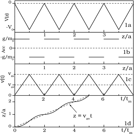
Figure 1: Plot of (a) potential, (b) acceleration, (c) velocity, and d) position for the electron motion in a saw-like potential (schematically).

It is seen from Fig. 1c that the velocity oscillates in time around the average value $v_{av}=v_{m}/2$. This is reflected in the oscillations of position $\Delta z(t)$ around the straight line $z=v_{av}t$, as seen in Fig. 1d. The latter are easily shown to be $\Delta z=\pm a/8$, which compares well with the classical results. Using the above estimation for $a$ we identify again the motion due to periodicity of the potential with the Zitterbewegung calculated previously with the use of two-band k.p model.

Strictly speaking, the physical sense of the above operator reasoning is reached when one calculates average values. Our procedure follows the original approach of Schrodinger Schroedinger30 , who integrated operator equations for $\hat{v}(t)$ and $\hat{z}(t)$. Similar approach is commonly used for $\hat{z}(t)$ and $\hat{p}(t)$ operators in the harmonic oscillator problem MessiahBook . Equation of motion (3) does not contain the total electron energy but it is clear from Fig. 1a that, in a quantum treatment, the electron can move either in allowed energy bands below the potential tops at $E\leq 0$ or above the tops at $E>0$.

Now we describe the ZB using a rigorous quantum approach. We employ the Kronig-Penney delta-like potential since it allows us to calculate explicitly the eigenenergies and eigenfunctions Kronig31 ; SmithBook . In the extended zone scheme the Bloch function is $\psi_{k}(z)=e^{ikz}A_{k}(z)$, where

$$A_{k}(z)=e^{-ikz}C_{k}\left\{e^{ika}\sin[\beta_{k}z]+\sin[\beta_{k}(a-z)]\right\},$$ (4)

in which $k$ is the wave vector, $C_{k}$ is a normalizing constant and $\beta_{k}=\sqrt{2m_{0}E}/\hbar$ is a solution of the equation

$$Z\frac{\sin(\beta_{k}a)}{\beta_{k}a}+\cos(\beta_{k}a)=\cos(ka),$$ (5)

with $Z>0$ being an effective strength of the potential. In the extended zone scheme, the energies $E(k)$ are discontinuous functions for $k=n\pi/a$, where $n=\ldots-1,0,1\ldots$. In this convention, if $n\pi/a\leq k\leq(n+1)\pi/a$, the energies $E(k)$ belong to the $n$-th band and the Bloch states are characterized by one quantum number $k$. Because $A_{k}(z)$ is a periodic function, one may expand it in the Fourier series $A_{k}(z)=\sum_{n}A_{n}\exp(ik_{n}z)$, where $k_{n}=2\pi n/a$.

In the Heisenberg picture the time-dependent velocity averaged over a wave packet $f(z)$ is

$$\langle\hat{v}(t)\rangle=\frac{\hbar}{m_{0}}\int\int\!\!dkdk^{\prime}\langle f|k\rangle\langle k|\frac{\partial}{i\partial z}|k^{\prime}\rangle\langle k^{\prime}|f\rangle e^{i(E_{k}-E_{k^{\prime}})t/\hbar},$$ (6)

where $|k\rangle$ is the Bloch state. The matrix elements of momentum are $\langle k|\hat{p}|k^{\prime}\rangle=\hbar\delta_{k^{\prime},k+k_{n}}K(k,k^{\prime})$, where

$$K(k,k^{\prime})=\int_{0}^{a}\psi_{k}(z)^{*}\frac{\partial\psi_{k^{\prime}}(z)}{i\partial z}dz,$$ (7)

The wave packet $f(z)$ is taken in a Gaussian form of the width $d$ and centered at $k_{0}$, and its matrix elements are $\langle f|k\rangle=\sum_{n}A_{n}F(k,k_{n})$, where

$$F(k,k_{n})=\int_{-\infty}^{\infty}f^{*}(z)e^{iz(k+k_{n})}dz.$$ (8)

Inserting the above matrix elements to Eq. (6) we obtain

$$\langle\hat{v}(t)\rangle=\frac{\hbar}{m_{0}}\sum_{n,n^{\prime},l}\int\int\!\!dkdk^{\prime}A^{*}_{n}A_{n^{\prime}}F^{*}(k,k_{n})F(k^{\prime},k_{n^{\prime}})\times$$

$$K(k,k^{\prime})e^{i(E_{k}-E_{k^{\prime}})t/\hbar}\delta_{k^{\prime},k+k_{l}}.$$ (9)

Figure 2 shows results for the electron ZB, as computed for a superlattice. The electron velocity and position are indicated. As follows from the inset in Fig. 3, a relative narrowness of the wave packet in $k$ space cuts down contributions from $k$ values away from $k_{0}$, and one deals effectively with the vicinity of one energy gap. It is seen that for a superlattice with the period $a=200$Å the ZB displacement is about $\pm 50$Å, i.e. a fraction of the period, in agrement with the rough estimations given above. The period of oscillations is of the order of several picoseconds.

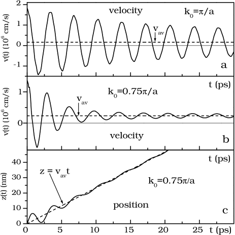
Figure 2: Calculated electron ZB velocities and position in a superlattice versus time. The packet width is $d=400$Å, Kronig-Penney parameter is $Z=1.5\pi$, superlattice period is $a=200$Å. (a) Packet centered at $k_{0}=\pi/a$; (b) and (c) packet centered at $k_{0}=0.75\pi/a$. The dashed lines indicate motions with average velocities.

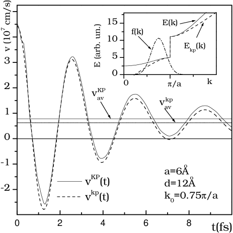
Figure 3: ZB of electron velocity in a periodic lattice versus time. Solid line: the complete Kronig-Penney model, dashed line: the two-band k.p model. Inset: Calculated bands for the Kronig-Penney (solid line) and the two-level k.p model (dashed line) in the vicinity of $k=\pi/a$. The wave packet $f(k)$ centered at $k_{0}=0.75\pi/a$ is also indicated (not normalized).

Finally, we want to demonstrate that the two-band k.p model, used until present to calculate the Zitterbewegung Rusin09 , is adequate for a description of this phenomenon. We calculate the packet velocity near the point $k_{0}=\pi/a$ for a one-dimensional Kronig-Penney periodic Hamiltonian using the Luttinger-Kohn (LK) representation Luttinger55 . The LK functions $\chi_{nk}(z)=e^{ikz}u_{nk_{0}}(z)$, where $u_{nk_{0}}(z)=u_{nk_{0}}(z+a)$, also form a complete set. We have

$$\langle\hat{v}(t)\rangle=\langle f|\hat{v}(t)|f\rangle=\sum_{kk^{\prime}nn^{\prime}}\langle f|nk\rangle\langle nk|\hat{v}(t)|n^{\prime}k^{\prime}\rangle\langle\ n^{\prime}k^{\prime}|f\rangle,$$ (10)

where the velocity in the Heisenberg picture is $\hat{v}(t)=(\hbar/m_{0})e^{i\hat{H}t/\hbar}(\partial/i\partial z)e^{-i\hat{H}t/\hbar}$. Restricting the above summation to the conduction and valence bands: $n,n^{\prime}=1,2$, we obtain in the matrix form

$$\langle\hat{v}(t)\rangle\approx\left(\begin{array}[]{c}f_{1}\\ f_{2}\end{array}\right)^{\dagger}\left(\begin{array}[]{cc}\hat{v}(t)_{11}&\hat{v}(t)_{12}\\ \hat{v}(t)_{21}&\hat{v}(t)_{22}\end{array}\right)\left(\begin{array}[]{c}f_{1}\\ f_{2}\end{array}\right),$$ (11)

where $f_{i}=\langle nk|f\rangle$, and $\hat{v}(t)_{nn^{\prime}}$ are the matrix elements of the time-dependent velocity operator between the LK functions. Equation (11) looks like the k.p approach to ZB used previously.

The k.p Hamiltonian is obtained from the initial periodic Hamiltonian in the standard way Luttinger55 ; Kane57 . In the two-band model the result is

$$\hat{H}_{kp}=\left(\begin{array}[]{cc}\hbar^{2}k^{2}/2m_{0}+E_{1}&\hbar kp_{21}/m_{0}\\ \hbar kp_{12}/m_{0}&\hbar^{2}k^{2}/2m_{0}+E_{2}\end{array}\right),$$ (12)

where $p_{12}=p_{21}^{*}$ are the interband elements of momentum, and $E_{1}$ and $E_{2}$ are the band-edge energies. The velocity matrix at $t=0$ is $\hat{v}_{kp}=\partial\hat{H}_{kp}/\hbar\partial k$. The calculation of velocity in the Heisenberg picture is described in Ref. Rusin07a .

In Fig. 3 we compare the ZB oscillations of velocity calculated using: (a) real $E(k)$ dispersions resulting from the Kronig-Penney model and the corresponding Bloch functions of Eq. (4); (b) two-band $E(k)$ dispersions obtained from Eq. (12) and the corresponding LK functions. It is seen that, although we take the packet not centered at $k=\pi/a$, the two-band k.p model gives an excellent description of ZB. For $k_{0}=\pi/a$ the two descriptions are almost identical. It is seen from Fig. 3 that for a wave packet of the width $d=2a$ the ZB is already well described by the k.p model. On the other hand, for a much wider packet in $k$ space the two descriptions differ more, especially when the $k$-width encompasses more than one energy gap.

A few remarks are in order. The transient character of ZB, illustrated in Figs. 2 and 3, is a result of describing the electron dynamics with the use of wave packets, see Lock79 . In particular, it is seen that wider packets (in real space) result in longer transient times. In the limiting cases of plane waves the electron oscillates indefinitely, similarly to the classical description Zawadzki05KP . Second, one should bear in mind that the standard conductivity theories use average electron velocities $\bar{v}=\hbar k/m^{*}$, as indicated in the above figures. Our work shows that at very short times the electron dynamics is completely different from its average behavior. Third, both periods and amplitudes of ZB, as shown in Fig. 2, are comparable to those appearing in the Bloch oscillation measurements Lyssenko96 , so the ZB should be also observable experimentally. Clearly, it is difficult to follow the behavior of a single electron and, in order to observe the trembling motion, one should produce many electrons moving in phase. This can be most readily done using laser pulses, see Rusin09 ; Lyssenko96 .

In summary, we considered fundamentals of electron motion in periodic structures and showed that the extensively studied phenomenon of electron Zitterbewegung in crystalline solids is caused by oscillations of velocity assuring the total energy conservation as an electron moves in a periodic potential. This means that, although the ZB in solids was often studied in literature using the two-band k.p model of band structure analogous to the Dirac equation for relativistic electrons in a vacuum, the origins of ZB in s solid and in a vacuum are completely different. We also performed a rigorous quantum calculation of ZB for an electron in the Kronig-Penney potential and showed that the two-band k.p model is adequate for its description.

We dedicate this work to the memory of Professor R. A. Smith, whose excellent book ”Wave Mechanics of Crystalline Solids” was very helpful in our endeavor. This work was supported in part by The Polish Ministry of Science and Higher Education through Laboratory of Physical Foundations of Information Processing.

References

- (1) E. Schrodinger, Sitzungsber. Preuss. Akad. Wiss. Phys. Math. Kl. 24, 418 (1930).
- (2) K. Huang, Am. J. Phys. 20, 479 (1952).
- (3) P. Krekora, Q. Su, and R. Grobe, Phys Rev. Lett. 93, 043004 (2004).
- (4) L. Ferrari and G. Russo, Phys. Rev. B 42, 7454 (1990).
- (5) S. W. Vonsovsky, M. S. Svirsky, and L. M. Svirskaya, Tieor. Matiem. Fizika. 94, 343 (1993) (in Russian).
- (6) W. Zawadzki, in High Magnetic Fields in the Physics of Semiconductors II, edited by G. Landwehr and W. Ossau (World Scientific, Singapore, 1997), p. 755.
- (7) W. Zawadzki, Phys. Rev. B 72, 085217 (2005).
- (8) J. Schliemann, D. Loss, and R. M. Westervelt, Phys. Rev. Lett. 94, 206801 (2005).
- (9) T. M. Rusin and W. Zawadzki, Phys. Rev. B 80, 045416 (2009) and references therein.
- (10) X. Zhang and Z. Liu, Phys. Rev. Lett. 101, 264303 (2008).
- (11) J. D. Bjorken and S. D. Drell, Relativistic Quantum Mechanics (McGraw-Hill, New York, 1964).
- (12) A. Messiah, Quantum Mechanics (North Holland, Amsterdam, 1961).
- (13) R. L. Kronig and W. Penney, Proc. Roy. Soc. London 130, 499 (1931).
- (14) R. A. Smith, Wave Mechanics of Crystalline Solids, (Chapman and Hall, London, 1961).
- (15) J. M. Luttinger and W. Kohn, Phys. Rev. 97, 869 (1955).
- (16) E. O. Kane, J. Phys. Chem. Solids 1, 249 (1957).
- (17) T. M. Rusin and W. Zawadzki, J. Phys. Cond. Matter 19, 136219 (2007).
- (18) J. A. Lock, Am. J. Phys. 47, 797 (1979).
- (19) V. G. Lyssenko et al., Phys. Rev. Lett. 79, 301 (1997).