Notes on disentangling of spectra

Abstract

Context. The determination of pulsation velocities from observed spectra of Cepheids is needed for the Baade-Wesselink calibration of these primary distance markers.

Aims. The applicability of the Fourier-disentangling technique for the determination of pulsation velocities of Cepheids and other pulsating stars is studied.

Methods. The KOREL-code was modified to enable fitting of free parameters of a prescribed line-profile broadening function corresponding to the radial pulsations of the stellar atmosphere. It was applied to spectra of $\delta$ Cep in the H-alpha region observed with the Ondřejov 2-m telescope.

Results. The telluric lines were removed using template-constrained disentangling, phase-locked variations of line-strengths were measured and the curves of pulsational velocities obtained for several spectral lines. It is shown that the amplitude and phase of the velocities and line-strength variations depend on the depth of line formation and the excitation potential.

Conclusions. The disentangling of pulsations in the Cepheid spectra may be used for distance determination.

1 Introduction

The method of Fourier disentangling of spectra was developed by Hadrava (1995) from the method of cross-correlation (cf., e.g., Hill 1993) to decompose, from a series of observed spectra of multiple stars, contributions of the individual components and to simultaneously find orbital parameters, or, more generally, to fit free parameters of the physics governing the Doppler shifts and line-profile variations. One of the advantages of disentangling compared to cross-correlation is that it does not require a template spectrum of a star with similar spectral type or a model atmosphere.

Zucker and Mazeh (2006) introduced their method of Template Independent RAdial-VELocity measurement (TIRAVEL) for single-lined spectroscopic binaries (SB1). Their method uses each exposure from a series of observations as a template for cross-correlation with all other exposures. Zucker and Mazeh mentioned that the KOREL-code (cf., e.g., Hadrava 2004b) for Fourier disentangling is also template-independent. Nevertheless, they advocated use of their TIRAVEL based on the alleged advantage that it assumes the individual radial velocities to be free variables not bounded by an orbital motion. However, KOREL enables the convergence of individual radial velocities of any component also. Moreover, KOREL can do this not only for SB1, which is an extremely simple case, but also for two or more components. The option of free velocities is rarely used, because in practice it is more advantageous to take the orbital motion of multiple stars into account and to solve directly for the orbital parameters. Zucker and Mazeh mentioned the case of a third component as an example of when free radial velocities are needed. However, just in this case the solving for orbital parameters of both the close and the wide orbit (taking into account also the light-time effect) simultaneously with the determination of radial velocities is advantageous, because it checks the consistency of the possibly small perturbation with the source spectra better than a two-step procedure of determination and subsequent solution of the radial-velocity curve.

One reason to solve in some cases for individual radial velocities independent of orbital motion is technical, e.g. in the case of an unreliable wavelength scale of the observed spectra, as it has been done in the study by Yan et al. (2008). However, a more important reason is seen in cases when the observed wavelength shifts of spectral lines are not due to overall orbital motion of the star but due to some other effects. One such case is the Doppler shift caused by pulsations of the stars. The use of Fourier disentangling in the spectroscopic studies of pulsating stars has been outlined by Hadrava (2004a,b). Here we shall demonstrate this method in practice in the case of the star $\delta$ Cep.

The study of either radially or non-radially pulsating stars is important as a clue to probe the inner structure of stars. In addition, the period-luminosity (PL) relation of Cepheids and some other radial pulsators is used as one of the few primary methods for distance determination. One needs to calibrate this PL-relation, and that can be done by the Baade-Wesselink method (Baade 1926, Wesselink 1946). In this method, the spectroscopically measured pulsation velocity is integrated over the course of the period to yield the changes of stellar radius, which, combined with photometric or interferometric variations, may reveal the distance to the star. However, the spectroscopic measurement is complicated by the line-profile variations caused not only by the radial motion of the stellar atmosphere (which must be integrated over the visible part of the stellar disc projected locally to the line of sight) but also due to changes of other physical conditions (e.g. the temperature and density) in line-forming regions of different lines. Consequently, the radial velocities $v_{r}$ measured by different methods reflect only indirectly the instantaneous pulsation velocity $v_{p}$ of the stellar surface. It is thus used to introduce the so called projection factor $p\equiv v_{p}/v_{r}$, which can be estimated either theoretically (e.g. Nardetto et al. 2004) or observationally (Nardetto et al. 2008 and citations therein). An alternative method directly matching the Doppler shifts and asymmetries of spectral lines with a proper model of line-profiles has been introduced by Gray and Stevenson (2007). Their approach is, in principle, equivalent to the above mentioned disentangling of pulsations (Hadrava 2004a,b).

We summarize the method of pulsation disentangling and its use in Sect. 2 and we test it on our observations of the $\delta$ Cep in Sect. 3. In Sect. 4 we discuss possibilities of further development of the method.

2 Disentangling of radial pulsations

The line-profile variations (LPVs) caused by motion of the stellar atmosphere are often modelled by integrating Doppler shifted spectra of unperturbed (mostly plane-parallel) model atmospheres over the stellar surface. This approximation is used for study of the rotational broadening as well as LPVs due to radial or non-radial pulsations even though it is obvious that the motion may change the structure of the atmosphere and hence also the radiative transfer and the line formation in them. In the case of Cepheids, it is observed that different lines formed in different layers of the atmosphere have slightly different phase-dependence of LPVs (cf. Breitfellner and Gillet 1993, Butler 1993 etc.), which reflects (besides other effects) the changes of velocity gradients within the atmosphere. The basic idea of the Baade-Wesselink method also assumes that the spectroscopic and photometric or interferometric variations are caused by pulsations of the same stellar surface. However, the dilution of the atmosphere and its temperature variations and the presence of stellar winds in these stars implies that the motion of layers with given optical depths may differ from the local velocity of the gas, which then influences the profiles and shifts of the spectral lines.

A safe way (outlined and followed, e.g., by A. Fokin, 1991, 2003 etc.) to treat all these effects properly would be to construct physically self-consistent models of atmospheres of pulsating stars, to calculate the observable quantities (spectra, light-curves, visibility functions) and to match the values of free parameters (including the distance) to the real data. However, the modelling itself is still computationally very demanding, not to speak of the inverse problem of solving for the free parameters. It is thus worth simultaneously following an alternative way of fitting the observations by simplified models, which take into account the most important effects and could be modified if a discrepancy with respect to self-consistent models or with respect to observations were found.

Let us assume now that the observed spectrum $I(x,t)$ (as a function of the logarithmic wavelength $x$ and time $t$) is given by the integral

$$I(x,t)=\int_{s}\mu I(x,s,\mu,t)\ast\delta(x-v(s,t))d^{2}s$$ (1)

over the visible part (i.e. where the directional cosine $\mu>0$) of the stellar surface $s$. If the specific intensity (in the rest frame of the moving atmosphere) is independent of $s$ and we expand it into a power series of $\mu$

$$I(x,s,\mu,t)=\sum_{k}I^{k}(x,t)\mu^{k}\;,$$ (2)

the spectrum is given by

$$I(x,t)=\sum_{k}I^{k}(x,t)\ast\Delta^{k}(x,t)\;,$$ (3)

where

$$\Delta^{k}(x,t)=\int_{s}\mu^{k+1}\delta(x-v(s,t))d^{2}s\;.$$ (4)

For purely radial pulsations synchronous on the whole stellar surface, the local radial velocity $v(s,t)=\mu v_{p}(t)$ is the projection of the instantaneous speed $v_{p}$ of the pulsation. The broadening functions for individual modes of the limb darkening then read

$$\Delta^{k}(x,t)=\frac{2\pi R^{2}}{v_{p}^{k+2}}\left[x^{k+1}\right]_{0}^{v_{p}}\;,$$ (5)

where $R=R(t)$ is the instantaneous radius of the star. The Doppler shift which can be measured by the first moment is given by the mean value of $x$ of the broadening and it reads

$$v_{r}\equiv\frac{\int x\Delta^{k}(x,t)dx}{\int\Delta^{k}dx}=\frac{k+2}{k+3}v_{p}\;.$$ (6)

In agreement with Getting (1934), the projection factor $p$ is thus $\frac{3}{2}$ for lines without limb darkening and $\frac{4}{3}$ with linear limb darkening equal to 1. For higher order terms of the series given by Eq. (2), the projection factor decreases toward the limiting value 1, which corresponds to the broadening function

$$\Delta^{\infty}(x,t)\sim\delta(x-v_{p}(t))\;,$$ (7)

i.e. to an absorption occurring in the centre of the stellar disc only. This calculation is valid exactly for radial-velocity measurement by the moment method only. For other methods, like the deepest point of the profile, bisectors, the fit by two semi-Gaussian curves or the cross-correlation method, the result of radial-velocity measurement of the asymmetric lines is less certain. It also depends on the instrumental broadening. Because the standard Fourier disentangling (which assumes the broadening function given by Eq. (7) only) is a handy method of radial-velocity measurement, it is worth investigating its properties (and its $p$-factor in particular) when applied to Cepheids, or modifying it by taking into account the proper broadening function so that it will avoid the $p$-factor completely and will directly provide the pulsational velocities.

It is generally understood that limb darkening is crucial for the asymmetry of the lines and thus also for setting the projection factor. However, determination of its proper value is still a problem (cf. Monta$\tilde{\rm n}$és Rodriguez and Jeffery 2001, Marengo et al. 2002). The limb-darkening corresponding to the radiation in continuum is sometimes accepted also in the lines, arguing that it “varies slowly with the wavelength and can be taken to be constant over the span of a spectral line” (Gray 2005, p. 436). However, the spectral flux in continuum also varies slowly with the wavelength, but it cannot be taken to be constant over any line because it is just its fast variation across the line-profile that is seen as the spectral lines. A simple model of radiative transfer in stellar atmospheres reveals that weak lines are usually dominated by the central part of the visible stellar disc and hence the differences between the radiation in the lines and in continuum has the limb darkening close to 1.0 (cf. Hadrava 1997). This is confirmed by the observed behaviour of the line strengths during eclipses and it is also consistent with the values $p\simeq 1.3$ of the projection factor in Cepheids. However, detailed non-LTE models of stellar atmospheres show that the limb darkening within strong lines (e.g. Balmer lines) is more complex (cf. Hadrava and Kubát 2003). It can be represented as a superposition of a part without limb darkening, a part with linear darkening, as well as of higher order terms, which also may include an emission (especially at the outer edges of the stellar disc if the spherical instead of the plane-parallel symmetry is taken into account). We shall thus investigate separately the cases of simulated pulsationally broadened lines without any limb darkening ($k=0$) and with linearly proportional broadening ($k=1$). We deconvolve these profiles (and in the next Section also real observed spectra) by disentangling with broadening functions for the same cases ($k=0,1$) and by the standard disentangling (i.e. $k=\infty$).

The generalization of disentangling for line-profile variability has been described by Hadrava (1997 and 1998 for the line-strength variability and the changes in shape of line-profile, respectively; unfortunately, the formulae were incorrectly processed in the print of the later paper). The explicit form of the pulsational broadening and its Fourier transform was given for the case of limb-darkening equal to 1 by Hadrava (2004a,b). The Fourier transform (from the space of functions of the variable $x$ to functions of $y$) of this profile (Eq. (5) for $k=1$) has the form

$$\tilde{\Delta}^{1}(y,t)=\frac{2\pi iR^{2}}{y^{3}v_{p}^{3}(t)}\left[\exp(iyv_{p})(2-2iyv_{p}-y^{2}v_{p}^{2})-2\right]\;.$$ (8)

Here we need also the case with zero limb-darkening ($k=0$), for which the Fourier transform reads

$$\tilde{\Delta}^{0}(y,t)=\frac{2\pi R^{2}}{y^{2}v_{p}^{2}(t)}\left[\exp(iyv_{p})(1-iyv_{p})-1\right]\;,$$ (9)

and also the standard disentangling, for which $\tilde{\Delta}^{\infty}(y,t)\simeq\exp(iyv_{p})$. The changes of $R(t)$ in these formulae influence the flux in the lines in absolute units proportionally also to the variations of the flux in continuum. Hence, they should not affect the line-strengths in the rectified spectrum (i.e. normalized to the continuum), unless there is also light from a binary companion or a background star present in the spectrum. However, because the changes of the effective temperature and other parameters of the stellar atmosphere in the course of the pulsational cycle generally affect the line-strengths, we substitute the term $2\pi R^{2}\equiv(k+2)s(t)$, where $s(t)$ is a multiplicative line-strength factor given by the integral of Eq. (5) over $x$ (which scales the broadening normalized to a unit integral).

We have calculated several sets of simulated data by direct integration in the $x$-space to always convolve one fixed Lorentzian line-profile ($\phi(x)\sim((x-x_{0})^{2}+\gamma^{2})^{-1}$) with broadening functions either $\Delta^{0}$ or $\Delta^{1}$ for instantaneous values of velocity $v_{p}(t)$ of a harmonic (i.e. sinusoidal) pulsation at 20 values of $t$ uniformly covering the period of the pulsation. The Lorentzian profile was chosen because it contains both a narrow core and wide wings. An example of such Lorentzian profiles with the intrinsic semi-halfwidth $\gamma$ corresponding to 30km/s broadened by $\Delta^{0}$ with a semi-amplitude of the pulsational velocity $K_{sim}$ equal to 100km/s is presented in Fig. 1. (The step of 100km/s is marked by the ticks on the $x$-axis.) It can be seen that the profiles (cf. the thick lines with offsets proportional to the phase) have the highest asymmetry at extremes of the pulsational velocity, the high-velocity wing always being steeper than the wider low-velocity wings reaching the rest wavelength of the line. Qualitatively the same feature also results if the pulsational broadening is applied to non-Lorentzian line profiles and is in agreement with the line-profile variations observed in Cepheids (cf., e.g., Breitfellner and Gillet 1993, Nardetto et al. 2006, Gray and Stevenson 2007). It is used to characterize such profiles quantitatively by bi-Gaussian fits (cf. Nardetto et al. 2006), which, however, are not physically substantiated.

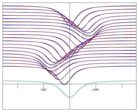
Figure 1: Standard disentangling (with $\Delta^{\infty}_{dis}$) of simulated Lorentzian profiles broadened by radial pulsations (with $\Delta^{0}_{sim}$, $q=0.3$). The simulated profiles are drawn by thick lines (blue in the electronic version), their fits using disentangling by thin (red) lines and the mean disentangled profile by the bottom (green) line.

Figure 1 also shows the disentangling of these simulated profiles by the standard KOREL disentangling (i.e. $\Delta^{\infty}$). For spectra containing lines of two or more component stars, the disentangling simultaneously decomposes them and fits the orbital parameters, while in the present case it leads to a simpler problem of fitting all the input spectra by a mean profile (which is drawn by the lowermost line) scaled in the line-strength and shifted in $x$. The best fits to the individual input profiles are overplotted in Fig. 1 by the thin lines. The disentangled mean profile is symmetric here (which need not be exactly the case if the pulsational velocity includes some higher overtones in addition to the basic sinusoidal mode, or if the spectra do not cover the period uniformly). Yet, it reproduces the input profiles relatively well, so that for real data the difference between the true profiles and the fit by a simplified model may be hidden in the noise. The coincidence is even better for input profiles broadened by $\Delta^{1}$ and disentangled by $\Delta^{\infty}$. In both cases the coincidence is worse if the amplitude of the pulsational velocity exceeds more the intrinsic width of the line. The disentangled profile is wider than the intrinsic profile (this is well seen e.g. in the uppermost input line, for which $v_{p}=0$), whenever the disentangling is performed using a smaller broadening (i.e. $\Delta^{k}$ with higher $k$) than the broadening used for the simulation of the data. If the input profiles are disentangled with the same broadening for which they were simulated, their fit as well as the reconstruction of the intrinsic profile is perfect within the numerical precision of the simulation. The disentangled line-strength factors are higher (up to nearly +0.08) for phases with low pulsational velocities and smaller (nearly $-0.08$) at extremes of the velocity.

The disentangling of this and other simulated datasets is performed here with velocities bound to a sinusoidal pulsation, which was also assumed in the creation of the data. This is done by formally assuming that the velocity obeys a circular motion. The ratio of the true amplitude $K_{sim}$ of the velocity chosen for the simulation and its disentangled value $K_{dis}$ gives a mean value of the projection factor $p$ for a particular combination of the broadening functions. The values of pulsational velocities which give the best fit of the mean disentangled profile with the individual input profiles are also calculated and they reveal that the projection factor is slightly phase-dependent. However, the differences are very small – in the particular case shown in Fig. 1 the free radial velocity is about 0.62km/s (i.e. nearly 1%) higher than the harmonic one at their extremes and about 0.47km/s lower at medium (non-zero) values of velocity. The profiles reconstructed with both velocities are drawn in Fig. 1 by the thin lines, but they are not distinguishable within the precision of the graphics. We thus neglect these differences which are of the order of the precision of the computation and we give the mean values of projection factors $p=K_{sim}/K_{dis}$ only for several combinations of broadening functions used for the simulation ($\Delta^{k}_{sim}$, $k=0,1$) and the disentangling ($\Delta^{k}_{dis}$, $k=0,1,\infty$) and the velocity-amplitude to line-width ratios $q=\gamma/K_{sim}$ in Table 1.

Table 1: Projection factors for simulated line-profiles

$$\begin{array}[]{rrrrrrrrr}\hline\cr\vskip 3.0pt plus 1.0pt minus 1.0pt\cr&&&\Delta^{0}_{sim}&&&&\Delta^{1}_{sim}&\\ \vskip 3.0pt plus 1.0pt minus 1.0pt\cr q&&\Delta^{0}_{dis}&\Delta^{1}_{dis}&\Delta^{\infty}_{dis}&&\Delta^{0}_{dis}&\Delta^{1}_{dis}&\Delta^{\infty}_{dis}\\ \vskip 3.0pt plus 1.0pt minus 1.0pt\cr\hline\cr\vskip 3.0pt plus 1.0pt minus 1.0pt\cr 0.1&&0.9999&1.0718&1.3942&&0.9426&0.9999&1.2556\\ 0.3&&0.9999&1.1074&1.4624&&0.9100&0.9999&1.3064\\ 1.0&&1.0001&1.1229&1.4945&&0.8918&1.0001&1.3297\\ 3.0&&1.0013&1.1262&1.5012&&0.8905&1.0015&1.3348\\ 10.&&1.0006&1.1253&1.5007&&0.8895&1.0003&1.3341\\ \vskip 3.0pt plus 1.0pt minus 1.0pt\cr\hline\cr\end{array}$$

It can be seen from these results that for lines broader than their Doppler shift ($q=\gamma/K_{sim}>1$) the standard disentangling (with $\Delta^{\infty}_{dis}$) yields $p$-factors agreeing within the numerical errors (which are of the order $10^{-3}$ here) with the moment method of the radial-velocity measurement, i.e. $\frac{4}{3}$ or $\frac{3}{2}$ for lines with unit ($\Delta^{1}_{sim}$) or zero ($\Delta^{0}_{sim}$) limb darkening. For lines with intrinsic widths $\gamma$ smaller than the pulsationally induced shifts and asymmetries, the standard disentangling is more sensitive to the position of the deeper parts of the profile and the $p$-factor decreases slightly closer to the value 1. The disentangling with the proper limb-darkening in the line (i.e. $\Delta^{1}_{dis}$ for $\Delta^{1}_{sim}$ and $\Delta^{0}_{dis}$ for $\Delta^{0}_{sim}$) has $p=1$, it means that it directly provides the pulsational velocities and it is desirable to use it for the Baade-Wesselink calibration. The use of improper broadening functions (i.e. $\Delta^{1}_{dis}$ for $\Delta^{0}_{sim}$ or vice versa), however, results in an error of about 10% in radial velocity. We thus need either to find the proper limb darkening across the line-profiles from detailed model atmospheres, or to distinguish which model fits the observed line-profiles better.

3 Disentangling of the observed spectra

To test the disentangling of pulsations on real data we started spectroscopic observations of $\delta$ Cep using the 700-mm camera of the spectrograph in the Coudé focus of the Ondřejov 2-m telescope equipped with LN2-cooled SITe CCD detector ST-005A (2030 $\times$ 800 15-$\mu$m pixels). Sixty nine medium-resolution spectra ($R\sim$ 13 000) with a linear dispersion of 17 Å/mm (0.25Å/pix) in H$\alpha$ region (6250–6770 Å) obtained between August 19, 2008 and April 16, 2009 (mostly by M. Šlechta) are used in this study. See on-line Table 3 or 4 for the journal of observations.

The spectra were reduced in IRAF using the standard packages ccdproc, doslit and rv (for more details of the processing see Škoda and Šlechta, 2002).

The spectral region around the H$\alpha$-line contains many atmospheric water-vapour lines which complicate the measurement of stellar spectra by standard methods (cf., e.g., Kiss and Vinkó 2000). However, Fourier disentangling with variable line strengths is not only suitable to remove the telluric lines (cf. Hadrava 1997, 2004a,b, 2006a), but at the same time it enables one to use them for an additional check or correction of the wavelength scale similarly to their use in classical methods (cf., e.g., Butler and Bell 1997). As the first step of the disentangling we chose the spectral region 6511–6521 Å sampled in 1024 bins (i.e. with a step in radial velocity of 0.45km/s per bin) to find the line-strength coefficients for the telluric lines. The Doppler shifts of the telluric lines with respect to the heliocentric wavelength-scale were calculated in the Keplerian approximation of the annual motion which is provided by the PREKOR-code from the coordinates of the target star (cf. Hadrava 2004b) and the telluric lines were disentangled by the standard disentangling using the broadening function $\Delta^{\infty}_{dis}$. The stellar lines in this region were disentangled as a superposition of two systems of lines using $\Delta^{1}_{dis}$ with free radial velocities and each one with its own free line-strength factors. To avoid uncertainties in low Fourier modes, which could cause anticorrelated distortions of the stellar and telluric component continua, we used disentangling constrained by a template (cf. Hadrava 2006b) for the telluric lines. The template had been calculated by disentangling spectra of the star 68u Her (i.e. spectroscopic binary HD 156633, also taken with the Ondřejov 2m-telescope), which gives a telluric spectrum with a satisfactorily flat continuum. The differences between the prescribed annual motion of the telluric lines and the radial velocities of these lines disentangled as the best fits of individual exposures were then used as corrections of the wavelength scale in the preparation of spectral regions for subsequent disentangling of the stellar lines. Owing to application of a method of enhanced precision (Hadrava 2009), these corrections were found with sub-pixel resolution. These wavelength corrections can be applied to exposures with sufficiently strong telluric lines only. In our case, the depth of telluric lines in exposures where they are weakest is about one half of their mean depth, so that the correction could be applied to all exposures.

Table 2: List of disentangled spectral lines

$$\begin{array}[]{rclrccr}\hline\cr\vskip 3.0pt plus 1.0pt minus 1.0pt\cr\lambda{\rm\leavevmode\nobreak\ [\AA]}\nobreak\leavevmode&rvpb&{\rm multiplet}&\chi+\varepsilon{\rm\leavevmode\nobreak\ [eV]}\nobreak\leavevmode&EW{\rm\leavevmode\nobreak\ [\AA]}\nobreak\leavevmode&v_{1}&s_{1}\\ \vskip 3.0pt plus 1.0pt minus 1.0pt\cr\hline\cr\vskip 3.0pt plus 1.0pt minus 1.0pt\cr 6265.14&0.7&{\rm Fe\leavevmode\nobreak\ I\leavevmode\nobreak\ (62)}&2.18&0.107&19.89&0.402\\ 6343.71&0.8&{\rm Ca\leavevmode\nobreak\ I\leavevmode\nobreak\ (53)}&4.44&0.184&20.40&0.531\\ 6347.10&0.7&{\rm Si\leavevmode\nobreak\ II\leavevmode\nobreak\ (2)}&8.15+8.12&0.245&18.88&-0.203\\ 6355.04&0.6&{\rm Fe\leavevmode\nobreak\ I\leavevmode\nobreak\ (342)}&2.83&0.110&19.82&0.508\\ 6358.69&0.6&{\rm Fe\leavevmode\nobreak\ I\leavevmode\nobreak\ (13)}&0.86&0.134&18.28&0.712\\ 6400.01&1.5&{\rm Fe\leavevmode\nobreak\ I\leavevmode\nobreak\ (816)}&3.60&0.263&21.42&0.319\\ 6456.39&0.8&{\rm Fe\leavevmode\nobreak\ II\leavevmode\nobreak\ (74)}&7.87+3.90&0.443&17.78&-0.069\\ 6663.45&1.0&{\rm Fe\leavevmode\nobreak\ I\leavevmode\nobreak\ (111)}&2.42&0.188&20.67&0.384\\ \vskip 3.0pt plus 1.0pt minus 1.0pt\cr\hline\cr\end{array}$$

To disentangle the pulsational velocities in the observed spectra of $\delta$ Cep we chose first several narrow spectral regions, each one containing a single dominant spectral line listed in Table 2. These regions were sampled in 256 bins each with a step of radial velocity per bin given in the Table ($rvpb$ in km/s). In some of the regions, blends with some weak lines can be seen, which partly decrease the quality of the disentangling, however, their influence can be neglected. The relatively low spectral resolution of our original data (about 12 km/s) provides only a rough sampling of line profiles in individual exposures, which have half-depth widths comparable to the amplitude of the Doppler shifts, i.e. only about 4 to 6 times larger. The disentangled line profiles are significantly smoother due to the averaging of a large number of the exposures. Nevertheless, the limited quality of the data does not enable us to convincingly decide which of the models $\Delta^{0}_{dis}$, $\Delta^{1}_{dis}$ and $\Delta^{\infty}_{dis}$ best fits the observed line-profile variations or even to search for their best linear combination, which could be expected for more general limb-darkening within the line-profile. We thus performed the disentangling of all regions for each of these models separately. In all regions, the integrated (O–C)² of the fitted spectra was the largest for the model $\Delta^{\infty}_{dis}$, while the residual noise for the pulsational broadenings $\Delta^{0}_{dis}$ and $\Delta^{1}_{dis}$ was nearly the same (within about 4%) without any evident regular preference of one model or the other. We thus illustrate the results on the case $\Delta^{1}_{dis}$, which corresponds to the unit limb darkening and is thus the most advantageous from the theoretical point of view (see above).

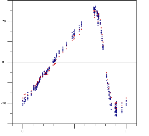
Figure 2: Phase-dependence of pulsational velocity $v$ in km/s for individual spectral lines disentangled with $\Delta^{1}_{dis}$. The phase $\phi$ is labeled in cycles (i.e. the non-integer part of the ephemeris $E$). Lines of neutral atoms are marked by open circles (blue in electronic version), lines of ionized atoms by (red) crosses.

Figure 2 shows the pulsational velocity disentangled using the model $\Delta^{1}_{dis}$ which is given in the on-line Table 3. For the purpose of visualizing the results (i.e. calculation of phase) we use the ephemeris

$$HJD=2454697.0009+5.366341\times E\;.$$ (10)

Our data do not allow us to check or improve the period, and the scatter in its published values (e.g. $P=5\aas@@fstack{d}{}3663159$ by Moffett and Barnes, 1985, or $5\aas@@fstack{d}{}3662351$ according to the quadratic ephemeris by Berdnikov and Ignatova, 2000) is not substantial for our present purpose. The reference epoch is chosen to closely precede our observations and coincide with the second exposure, which is relatively close to the minimum radial velocity.

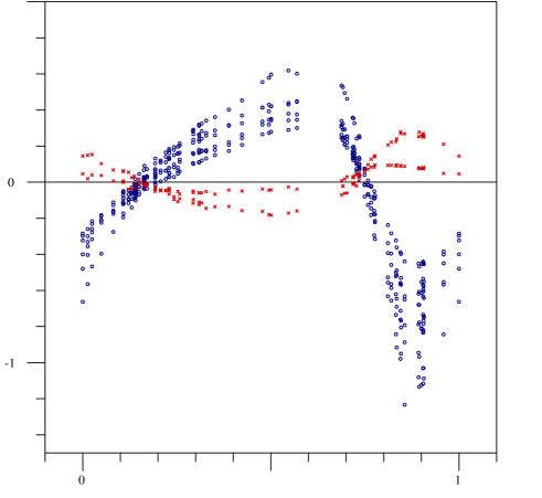
Figure 3: Phase-dependence of line-strength factors $s$ for individual spectral lines disentangled with $\Delta^{1}_{dis}$. (The meaning of symbols is the same as in Fig. 2.)

3

Table 3: Pulsational velocities $v$ for individual lines (cf. Table 2) and H$\alpha$ region at all exposures.

$$\begin{array}[]{rrrrrrrrrrrrr}\hline\cr\vskip 3.0pt plus 1.0pt minus 1.0pt\cr\begin{array}[]{c}{\rm HJD}\\ -2454000\end{array}&{\rm phase}&6265.14&6343.71&6347.10&6355.04&6358.69&6400.01&6456.39&6663.45&H_{\alpha\,1}&H_{\alpha\,2}&H_{\alpha\,3}\\ \vskip 3.0pt plus 1.0pt minus 1.0pt\cr\hline\cr\vskip 3.0pt plus 1.0pt minus 1.0pt\cr 698.3027&.2426&-3.472&-4.805&-3.114&-4.231&-3.812&-3.377&-5.866&-4.813&-10.724&-3.538&-3.581\\ 702.3672&.0000&-19.120&-20.131&-18.591&-18.690&-18.623&-21.070&-17.497&-20.683&-20.926&-18.053&-21.937\\ 708.4863&.1403&-10.826&-10.841&-9.845&-10.457&-9.998&-10.685&-10.559&-11.224&-16.223&-9.298&-10.475\\ 708.4925&.1414&-10.311&-11.554&-9.525&-11.006&-10.281&-9.949&-9.568&-10.841&-16.093&-8.544&-10.079\\ 709.3067&.2932&.463&.161&.131&.168&.355&1.027&-1.491&.367&-6.903&-.535&.282\\ 709.3918&.3090&.541&1.024&.803&.661&1.017&2.076&-.660&1.090&-5.914&.429&1.306\\ 709.4934&.3279&3.044&3.655&2.640&2.909&2.310&3.953&1.411&3.139&-3.749&2.340&3.406\\ 710.2962&.4775&11.764&13.170&12.519&12.540&11.533&14.355&10.445&12.580&6.654&10.167&13.655\\ 710.3885&.4947&12.200&14.001&12.923&13.476&11.755&15.001&11.141&13.225&7.582&10.522&14.431\\ 713.3641&.0492&-16.299&-18.433&-15.865&-17.112&-14.856&-17.865&-15.884&-17.800&-21.821&-14.746&-17.823\\ 719.2701&.1498&-9.941&-10.207&-9.739&-9.979&-9.482&-10.167&-9.862&-10.687&-16.053&-9.057&-9.976\\ 719.3365&.1622&-8.472&-9.176&-8.075&-8.449&-7.727&-8.343&-8.468&-9.273&-14.641&-7.795&-8.541\\ 719.3823&.1707&-8.104&-6.857&-7.089&-6.962&-7.039&-7.396&-7.464&-8.359&-13.749&-7.148&-7.656\\ 719.4983&.1923&-6.140&-5.839&-5.920&-5.720&-5.739&-5.189&-5.965&-7.151&-12.214&-5.771&-5.955\\ 719.5025&.1931&-7.041&-6.427&-6.718&-6.484&-6.072&-6.175&-6.978&-7.242&-13.088&-6.391&-6.643\\ 719.5764&.2069&-5.763&-6.034&-4.739&-4.705&-4.399&-4.846&-6.002&-5.864&-11.677&-5.091&-5.187\\ 736.4506&.3513&5.086&4.986&4.263&4.868&4.232&5.656&2.834&4.452&-2.272&4.177&5.114\\ 737.2522&.5007&14.810&14.151&12.956&13.590&12.394&15.191&11.347&15.769&9.054&11.995&15.898\\ 737.4991&.5467&15.897&16.675&15.857&15.609&14.873&17.766&13.501&16.647&11.422&13.820&18.197\\ 737.6202&.5693&18.153&18.430&17.510&17.579&16.354&19.509&15.891&18.914&13.497&15.659&20.182\\ 738.2559&.6877&25.667&26.431&25.142&26.082&24.013&26.733&24.830&26.803&21.757&23.688&27.721\\ 738.3353&.7025&25.542&26.555&24.756&25.440&24.145&26.485&25.407&27.217&23.200&24.194&28.507\\ 738.4407&.7222&22.621&24.298&22.876&23.889&22.326&24.393&24.408&23.966&23.626&22.297&27.316\\ 738.5058&.7343&21.891&22.284&22.006&22.177&21.452&22.448&23.506&23.296&24.665&20.887&26.895\\ 738.5121&.7355&22.000&22.983&21.673&22.090&21.350&22.549&23.257&23.523&24.795&20.794&26.921\\ 738.5852&.7491&18.959&19.164&18.943&19.028&18.171&18.670&20.746&20.229&24.993&18.405&24.877\\ 744.3990&.8325&-12.053&-12.730&-12.948&-13.166&-10.740&-14.169&-10.648&-14.182&15.896&-11.724&-16.115\\ 751.2407&.1074&-13.394&-13.437&-12.515&-12.752&-12.051&-13.271&-11.996&-13.347&-17.913&-11.563&-13.046\\ 751.2445&.1081&-13.639&-12.864&-11.994&-12.394&-11.397&-12.946&-11.251&-12.639&-17.725&-11.017&-12.618\\ 752.2419&.2940&-.351&-.150&-.213&-.023&-.118&.540&-1.416&.192&-7.474&.391&.310\\ 752.3239&.3093&.104&.517&.161&.235&.368&1.205&-1.246&.242&-6.694&.390&.755\\ 752.3612&.3162&.601&.873&.901&.883&1.079&1.952&-.628&.618&-5.854&.430&1.406\\ 757.2615&.2294&-4.640&-4.563&-4.879&-4.458&-4.136&-4.008&-5.363&-4.740&-11.266&-4.572&-4.490\\ 758.3017&.4232&8.058&8.891&8.077&8.648&7.927&9.663&6.442&8.495&2.435&6.836&9.369\\ 761.4677&.0132&-19.167&-19.361&-17.262&-17.943&-17.526&-19.989&-15.940&-19.126&-22.674&-15.931&-20.340\\ 771.2950&.8445&-16.757&-18.029&-17.489&-17.553&-14.807&-20.774&-15.062&-18.224&10.474&-15.843&-21.765\\ 771.3017&.8457&-17.270&-17.912&-17.540&-18.093&-17.744&-20.982&-14.826&-18.092&9.583&-16.326&-22.067\\ 772.2613&.0245&-18.332&-18.172&-17.079&-18.665&-17.204&-19.081&-15.587&-18.398&-21.602&-15.372&-19.205\\ 774.2135&.3883&6.001&5.869&5.153&5.797&5.404&7.304&4.523&6.392&-.147&5.395&7.202\\ 776.1982&.7582&14.591&15.493&14.505&14.258&14.348&13.684&16.629&15.125&23.436&14.231&21.215\\ 776.2430&.7665&11.360&11.644&11.325&11.487&10.499&10.375&13.564&12.644&23.432&11.784&18.674\\ 776.2868&.7747&7.889&7.464&7.835&7.097&7.709&6.312&10.046&8.428&22.699&8.657&14.885\\ 776.2972&.7766&7.360&6.757&7.886&7.655&7.222&6.257&9.713&8.030&23.566&8.493&14.584\\ 781.2311&.6960&24.209&24.341&21.721&23.887&22.540&24.820&23.302&25.921&21.316&22.742&26.844\\ 798.3846&.8925&-22.209&-20.912&-22.504&-22.707&-24.052&-26.179&-20.384&-24.487&-4.586&-21.204&-28.487\\ 798.3939&.8943&-22.432&-21.594&-21.541&-21.999&-20.465&-25.455&-19.844&-23.852&-4.747&-20.621&-27.909\\ 798.4495&.9046&-22.934&-23.639&-22.419&-23.410&-20.900&-26.265&-20.292&-24.475&-7.728&-21.228&-28.217\\ 824.3317&.7277&18.792&20.530&17.753&18.852&17.995&19.383&19.651&20.842&20.695&16.979&23.366\\ 843.2488&.2528&-2.825&-2.918&-3.969&-3.555&-2.882&-2.933&-4.288&-2.926&-10.146&-2.626&-2.791\\ 857.2159&.8555&-20.871&-20.889&-20.036&-20.335&-20.987&-23.105&-17.185&-20.980&5.365&-19.282&-25.892\\ 910.6409&.8111&-7.020&-7.160&-6.173&-6.396&-5.840&-9.023&-5.008&-7.355&20.318&-5.737&-6.244\\ 923.5714&.2207&-5.783&-5.871&-5.055&-5.467&-5.484&-5.258&-6.204&-5.840&-12.770&-5.549&-5.808\\ 923.6211&.2299&-5.610&-5.789&-4.929&-5.372&-5.455&-4.547&-6.149&-5.344&-12.815&-5.218&-5.527\\ 927.5339&.9591&-23.305&-22.027&-21.087&-23.797&-19.956&-24.735&-19.891&-23.971&-21.156&-19.528&-25.434\\ 928.4066&.1217&-12.945&-13.761&-11.411&-12.335&-12.105&-13.326&-12.596&-12.991&-18.469&-10.608&-12.469\\ 928.4523&.1302&-12.809&-13.317&-10.827&-11.937&-11.876&-12.539&-11.972&-13.189&-18.086&-10.433&-12.017\\ 928.4885&.1370&-12.083&-12.143&-10.498&-11.798&-11.156&-11.789&-11.150&-12.400&-17.737&-10.201&-11.629\\ 928.6318&.1637&-9.680&-9.726&-9.079&-9.399&-9.103&-9.293&-9.046&-9.384&-14.967&-8.243&-8.868\\ 931.4636&.6914&25.727&25.717&24.632&26.043&24.502&26.672&25.196&26.687&21.251&23.321&27.381\\ 931.6042&.7176&24.333&24.484&22.787&24.512&22.557&24.579&24.155&25.221&23.197&22.469&27.464\\ 931.6139&.7194&23.349&23.641&22.779&23.520&22.059&23.678&23.775&24.484&23.100&21.896&27.099\\ 932.5844&.9002&-22.441&-22.897&-22.678&-23.743&-20.409&-25.682&-19.925&-24.120&-7.148&-20.443&-27.991\\ 932.6097&.9049&-23.106&-24.767&-22.705&-23.376&-20.218&-25.918&-19.832&-24.021&-8.526&-20.536&-27.756\\ 932.6138&.9057&-23.617&-25.700&-22.690&-23.541&-22.236&-26.092&-19.773&-23.632&-8.680&-20.248&-27.686\\ 932.6178&.9064&-21.966&-24.284&-22.814&-23.471&-19.347&-26.057&-20.040&-24.018&-8.634&-20.353&-27.959\\ 933.5557&.0812&-15.562&-15.682&-15.102&-15.644&-14.291&-16.345&-14.030&-15.348&-20.031&-12.778&-15.282\\ 934.5024&.2576&-3.043&-3.294&-2.396&-2.486&-3.021&-2.173&-4.223&-2.895&-10.500&-2.929&-2.991\\ 937.5199&.8199&-10.328&-12.313&-10.500&-10.560&-10.105&-13.348&-8.644&-11.404&16.376&-9.508&-11.648\\ 937.5973&.8344&-14.296&-15.723&-15.037&-15.085&-14.187&-17.760&-12.443&-16.271&12.039&-13.840&-18.320\\ \vskip 3.0pt plus 1.0pt minus 1.0pt\cr\hline\cr\end{array}$$

The fit of the observed spectra by the standard disentangling ($\Delta^{\infty}_{dis}$) is invariant with respect to adding a constant to all disentangled radial velocities and a simultaneous shift of the disentangled spectrum in the logarithmic wavelength for the corresponding value. If the position of the stellar spectrum disentangled from all exposures (transformed first into heliocentric wavelength scale) is fixed to the laboratory wavelengths of identified stellar lines, the measured radial velocities correspond to instantaneous heliocentric radial velocities. Neglecting the systematic errors caused by the line-profile distortions, the heliocentric radial velocity of the star could be estimated as the velocity averaged over the pulsational period

$$\bar{v}\equiv\frac{1}{P}\int_{0}^{P}v(t)dt\;.$$ (11)

Having the values of velocities measured with some errors in several discrete times only, we fit them using least-squares method in the standard manner by Fourier series (cf. Schaltenbrand and Tammann 1971, or Moffett and Barnes 1985, etc.)

$$v(t)\simeq v_{0}+\sum_{k=1}^{K}v_{k}\sin(2\pi kt/P+\phi_{k})\;.$$ (12)

The mean velocity $\bar{v}$ is then given by the first term $v_{0}$. We have chosen $K=5$, because the residual $(O-C)^{2}$ of the fit decreased significantly with each additional harmonic term up to this value, but its value remains practically constant (given by the rms. error of the measurements) for higher degree of the expansion. We also used the same Fourier series for the line-strength factors.

Unlike the standard disentangling, the disentangling with broadening functions $\Delta^{0}_{dis}$ and $\Delta^{1}_{dis}$ is sensitive to the value of the true radial velocity of the star’s centre of mass. At the phases when the pulsational velocity is equal to zero, the consequent line-profile distortion disappears, the instantaneous line-profile coincides (within the errors) with the disentangled one and its Doppler shift is given by the overall motion of the star only. The Doppler shift of the disentangled spectrum should thus correspond to the intrinsic radial velocity of the star. However, because a systematic shift of all pulsational velocities can be relatively well compensated by a shift of the disentangled spectrum, the convergence of the solution to the true radial velocity is very slow and the value of the velocity is poorly defined, in particular for the rough sampling of the line profiles in our spectra. (To speed up the convergence we introduced an additive term in the velocity, which is possible to converge explicitly by the simplex method.) The values for which we achieve the best fit of the observed spectra differ somewhat from the values $v_{0}$ found from the fit by Eq. (12). This discrepancy may be due to the mentioned observational errors, but it may also reflect an influence of effects neglected in the simple models given by the broadening functions $\Delta^{0}_{dis}$ and $\Delta^{1}_{dis}$. For instance the gradients of pulsational velocities or the stellar wind overimposed on the pulsations may contribute a distortion resembling P-Cyg shape to the line profile. More precise measurements as well as models of line formation will be needed to solve this question.

In Table 2 we give the amplitude $v_{1}$ of the first periodic term in the expansion given by Eq. (12). It can be seen that this amplitude is smaller for the lines of ionized elements and it is slightly correlated with the equivalent width of the lines of neutral elements. This result indicates that the amplitude of pulsational velocities depends on the depth in the atmosphere where the line is formed (cf. Butler et al. 1996, Petterson et al. 2005, and references therein). This also qualitatively agrees with the correlation between line-depths and amplitudes of radial-velocity curves found in Cepheids by Nardetto et al. (2007 and 2009).

4

Table 4: Line-strength factors for individual lines (cf. Table 2) and H$\alpha$ region at all exposures.

$$\begin{array}[]{rrrrrrrrrrrrr}\hline\cr\vskip 3.0pt plus 1.0pt minus 1.0pt\cr\begin{array}[]{c}{\rm HJD}\\ -2454000\end{array}&{\rm phase}&6265.14&6343.71&6347.10&6355.04&6358.69&6400.01&6456.39&6663.45&H_{\alpha\,1}&H_{\alpha\,2}&H_{\alpha\,3}\\ \vskip 3.0pt plus 1.0pt minus 1.0pt\cr\hline\cr\vskip 3.0pt plus 1.0pt minus 1.0pt\cr 698.3027&.2426&.0822&.1945&-.0958&.1495&.1788&.0290&-.0812&.0981&.1646&-.0497&-.0258\\ 702.3672&.0000&-.3228&-.3998&.1446&-.4800&-.6630&-.2845&.0459&-.2972&-.5038&.1219&.0517\\ 708.4863&.1403&-.0631&.0173&-.0047&-.0120&-.1017&-.0843&-.0182&-.0507&-.0129&.0160&.0057\\ 708.4925&.1414&-.0621&-.0422&-.0268&-.0314&-.0726&-.0748&-.0320&-.0200&-.0290&.0138&.0024\\ 709.3067&.2932&.1607&.2827&-.1163&.2193&.2876&.1056&-.0488&.1595&.2507&-.0651&-.0263\\ 709.3918&.3090&.1620&.2648&-.1247&.2376&.3187&.1084&-.0597&.1801&.2522&-.0712&-.0312\\ 709.4934&.3279&.1702&.2728&-.1448&.2580&.3411&.1310&-.0519&.1772&.2757&-.0802&-.0356\\ 710.2962&.4775&.3363&.4138&-.1619&.4130&.5553&.2653&-.0381&.3183&.4408&-.1235&-.0453\\ 710.3885&.4947&.3457&.4286&-.1795&.3925&.5778&.2728&-.0447&.3195&.4484&-.1263&-.0475\\ 713.3641&.0492&-.2249&-.2079&.1028&-.2110&-.3964&-.1825&.0373&-.1871&-.2661&.0813&.0378\\ 719.2701&.1498&-.0248&.0455&.0164&-.0269&-.0686&-.0543&-.0114&-.0041&.0258&.0100&.0055\\ 719.3365&.1622&-.0085&.0665&-.0107&.0285&.0198&-.0346&-.0035&.0099&.0585&.0068&.0061\\ 719.3823&.1707&-.0118&.0725&-.0072&.0273&.0343&-.0359&-.0136&.0258&.0646&-.0012&-.0001\\ 719.4983&.1923&.0241&.1042&-.0507&.0600&.0720&-.0009&-.0390&.0466&.1049&-.0176&-.0089\\ 719.5025&.1931&.0314&.1309&-.0362&.0719&.0455&-.0135&-.0307&.0359&.1078&-.0157&-.0061\\ 719.5764&.2069&.0527&.1196&-.0483&.1092&.1192&.0041&-.0419&.0652&.1261&-.0264&-.0130\\ 736.4506&.3513&.1779&.2870&-.1361&.2601&.3609&.1495&-.0662&.1972&.2877&-.0917&-.0421\\ 737.2522&.5007&.3512&.4208&-.1832&.4199&.5960&.2792&-.0423&.3434&.4505&-.1257&-.0469\\ 737.4991&.5467&.3798&.4295&-.1712&.4397&.6185&.2893&-.0264&.3426&.4776&-.1349&-.0505\\ 737.6202&.5693&.3756&.4485&-.1599&.4454&.6012&.3005&-.0385&.3456&.4745&-.1365&-.0540\\ 738.2559&.6877&.3053&.3395&-.0703&.3159&.5363&.2469&.0079&.2631&.4079&-.0913&-.0403\\ 738.3353&.7025&.2544&.2399&-.0595&.2531&.4621&.1909&.0302&.2182&.3824&-.0810&-.0408\\ 738.4407&.7222&.1818&.1591&-.0076&.1638&.3267&.1410&.0368&.1314&.3433&-.0588&-.0372\\ 738.5058&.7343&.1359&.0316&.0093&.0895&.2559&.1008&.0392&.0850&.3233&-.0448&-.0369\\ 738.5121&.7355&.1265&.0375&.0330&.0729&.2478&.1011&.0511&.0796&.3302&-.0435&-.0353\\ 738.5852&.7491&.0666&-.0804&.0751&-.0164&.0764&.0393&.0582&-.0128&.2784&-.0145&-.0283\\ 744.3990&.8325&-.5208&-.7354&.2252&-.6206&-.8432&-.3233&.0891&-.5007&-.5875&.2436&.1080\\ 751.2407&.1074&-.1120&-.0517&.0590&-.1096&-.1948&-.1219&-.0007&-.0718&-.0941&.0380&.0145\\ 751.2445&.1081&-.0881&-.0494&.0627&-.0886&-.1729&-.1202&.0065&-.0581&-.0913&.0377&.0150\\ 752.2419&.2940&.1563&.2657&-.0964&.2344&.2906&.1015&-.0583&.1596&.2276&-.0672&-.0287\\ 752.3239&.3093&.1694&.2572&-.1106&.2262&.3124&.1120&-.0581&.1696&.2443&-.0740&-.0329\\ 752.3612&.3162&.1713&.2825&-.1142&.2405&.3249&.1205&-.0593&.1746&.2609&-.0765&-.0336\\ 757.2615&.2294&.0788&.1843&-.0666&.1306&.1272&.0300&-.0417&.0791&.1495&-.0353&-.0166\\ 758.3017&.4232&.2640&.3692&-.1577&.3261&.4534&.2066&-.0491&.2440&.3620&-.1138&-.0507\\ 761.4677&.0132&-.3306&-.4034&.1500&-.3557&-.5652&-.2592&.0193&-.2993&-.4691&.1000&.0386\\ 771.2950&.8445&-.5584&-.7611&.2783&-.7125&-.9788&-.3885&.0890&-.5658&-.8165&.2429&.1093\\ 771.3017&.8457&-.5683&-.8052&.2690&-.7677&-.9505&-.3981&.0913&-.5304&-.8146&.2429&.1100\\ 772.2613&.0245&-.2594&-.2781&.1527&-.3165&-.4674&-.2314&.0402&-.2163&-.4133&.1053&.0466\\ 774.2135&.3883&.2071&.3127&-.1345&.3166&.4022&.1728&-.0439&.2210&.3391&-.1006&-.0412\\ 776.1982&.7582&-.0143&-.1265&.0966&-.0651&-.0183&.0098&.0719&-.0697&.2625&.0126&-.0146\\ 776.2430&.7665&-.0260&-.1824&.1273&-.1452&-.0833&-.0207&.0843&-.1136&.2290&.0452&.0006\\ 776.2868&.7747&-.0914&-.2949&.1402&-.1773&-.1585&-.0507&.0838&-.1767&.1790&.0836&.0207\\ 776.2972&.7766&-.0859&-.3156&.1466&-.2221&-.2148&-.0736&.0954&-.1786&.1704&.0951&.0262\\ 781.2311&.6960&.2466&.2483&-.0620&.2925&.4941&.2083&.0174&.2111&.3797&-.0863&-.0433\\ 798.3846&.8925&-.6794&-.9454&.2519&-.7883&-1.0806&-.4518&.0747&-.6174&-1.1268&.2184&.0990\\ 798.3939&.8943&-.6798&-.9679&.2774&-.7770&-1.1335&-.4669&.0799&-.6073&-1.1220&.2183&.0995\\ 798.4495&.9046&-.6331&-.8344&.2701&-.7342&-1.0309&-.4408&.0748&-.5710&-1.0990&.2093&.0942\\ 824.3317&.7277&.1312&.0625&-.0206&.1002&.2414&.1081&.0435&.0733&.3419&-.0566&-.0400\\ 843.2488&.2528&.0637&.1961&-.1087&.1569&.1600&.0467&-.0507&.0811&.1681&-.0553&-.0287\\ 857.2159&.8555&-.6509&-.8872&.2686&-.7922&-1.2336&-.4391&.0873&-.6319&-.9423&.2389&.1094\\ 910.6409&.8111&-.3374&-.5566&.2064&-.5274&-.6323&-.2376&.0936&-.3928&-.2223&.2320&.1034\\ 923.5714&.2207&.0640&.1649&-.0442&.1104&.1402&.0178&-.0479&.0640&.1309&-.0367&-.0191\\ 923.6211&.2299&.0494&.1752&-.0479&.1604&.1351&.0278&-.0341&.0519&.1435&-.0438&-.0223\\ 927.5339&.9591&-.4009&-.5680&.2103&-.5540&-.8438&-.3840&.0482&-.4500&-.8135&.1525&.0638\\ 928.4066&.1217&-.0681&-.0455&.0547&-.0924&-.1163&-.0973&-.0391&-.0687&-.0858&.0124&-.0046\\ 928.4523&.1302&-.0665&-.0292&.0253&-.0592&-.1405&-.0934&-.0359&-.0576&-.0593&.0078&-.0055\\ 928.4885&.1370&-.0520&-.0104&.0332&-.0482&-.0913&-.0898&-.0403&-.0325&-.0387&.0029&-.0076\\ 928.6318&.1637&-.0262&.0903&.0027&.0230&.0079&-.0384&-.0236&.0081&.0404&-.0035&-.0049\\ 931.4636&.6914&.2908&.2347&-.0218&.3235&.5266&.2320&-.0214&.2465&.3901&-.1184&-.0646\\ 931.6042&.7176&.1931&.1321&-.0038&.1705&.3577&.1551&.0246&.1518&.3506&-.0804&-.0511\\ 931.6139&.7194&.1966&.1212&-.0128&.1721&.3544&.1502&.0286&.1391&.3499&-.0775&-.0501\\ 932.5844&.9002&-.6140&-.8125&.2560&-.8086&-1.1247&-.4521&.0753&-.5533&-1.1375&.2081&.0925\\ 932.6097&.9049&-.5955&-.8288&.2492&-.8191&-1.1159&-.4518&.0821&-.5350&-1.0868&.2048&.0914\\ 932.6138&.9057&-.6062&-.7851&.2597&-.7683&-1.0302&-.4456&.0788&-.5772&-1.1177&.2054&.0916\\ 932.6178&.9064&-.6428&-.7434&.2541&-.7506&-1.0873&-.4546&.0782&-.5523&-1.1196&.2050&.0915\\ 933.5557&.0812&-.1641&-.1123&.0679&-.1756&-.2754&-.1572&.0065&-.1275&-.1884&.0491&.0165\\ 934.5024&.2576&.1131&.2151&-.0909&.1636&.2027&.0592&-.0651&.1253&.1865&-.0594&-.0291\\ 937.5199&.8199&-.3956&-.5863&.2219&-.5648&-.6562&-.2838&.0934&-.4585&-.3727&.2369&.1075\\ 937.5973&.8344&-.5158&-.6904&.2402&-.6457&-.9161&-.3619&.0952&-.4885&-.6210&.2414&.1099\\ \vskip 3.0pt plus 1.0pt minus 1.0pt\cr\hline\cr\end{array}$$

Similarly, the line-strength factors (see Fig. 3 and on-line Table 4) of the lines were expanded into the Fourier series and the amplitudes $s_{1}$ of the first component are also given in Table 2. The negative values of this amplitude are assigned to the lines which are approximately in an antiphase with the other lines. These are the two lines of ionized elements in our set, for which $\phi_{1}\simeq-35^{\circ}$, while for the lines of neutral atoms we have $\phi_{1}\simeq 165^{\circ}$. This amplitude (anti-)correlates well with the excitation potential $\varepsilon$ (+ ionization potential $\chi$, cf. Moore et al. 1966) of the lower level of the line. The largest deviation can be seen for the Ca I line, which, however, may be blended with the Fe I (169) line 6344.15 Å with $\varepsilon=2.42$ eV. These variations of line strengths measured by the method of relative line photometry (Hadrava 1997) thus enable one to easily find the changes of atmosphere temperature in the course of the Cepheid pulsation period (cf. Krockenberger et al., 1998, Kovtyukh and Gorlova 2000).

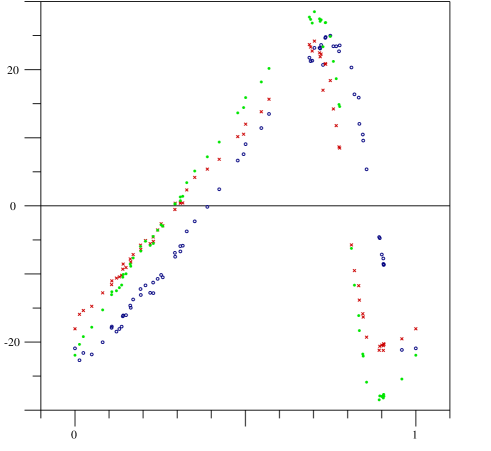
Figure 4: Phase-dependence of pulsational velocity in km/s for spectral lines in the H$\alpha$ region. The one-component solution is marked by (green) full circles, low- and high- excitation components of the two-component disentangling are marked by (blue) open circles and (red) crosses, resp.

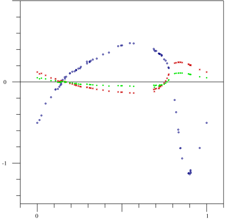
Figure 5: Phase-dependence of line-strength factors $s$ for spectral lines in the H$\alpha$ region. (The meaning of symbols is the same as in Fig. 4.)

As a next step we performed disentangling of a wide spectral region (6506–6618 Å) around the H$\alpha$ line. We chose sampling in 1024 bins with a step of 5km/s per bin. The telluric lines were disentangled using a template obtained from spectra of 68u Her again. The pulsational velocities and line-strength factors obtained by disentangling of the whole spectral region into one stellar component are given in Tables 3 and 4 (in columns labeled H_α 3) and drawn (by full circles in green) in Fig. 4 and 5, respectively. The semiamplitude of the first Fourier mode of the pulsational velocity is $v_{1}=21.40$ km/s; the line-strength factors have a semiamplitude $s_{1}=0.062$ and phase shift ($\phi_{1}\simeq-20^{\circ}$) comparable to that of the ionized atoms in Fig. 3. The phase dependence of residual spectra is drawn in Fig. 6. (The wavelength $\lambda$ is drawn on a logarithmic scale and labeled in Å.) It can be seen here that the strength of the H$\alpha$ wide wings is almost in antiphase with its narrow core as well as with strengths of weaker metallic lines. The residuals in the wings are thus in absorption and the narrow lines in emission around phase 0.0 around maximum expansion (cf. the bottom and uppermost lines) and it is reversed around phase 0.5 at the infall (the lines around the middle of the Figure). Residuals of some of the narrow lines have a shape of P-Cyg or inverse P-Cyg profiles in some phases. This indicates that the Doppler shifts of these lines differ from the other lines.

Figure 6: Residual spectra in the H$\alpha$ region after 1-component (+ telluric spectrum) disentangling. The vertical offset is proportional to the phase.

To decrease the residual spectrum, we must allow each line to vary its line strengths in agreement with the phase-locked changes of the atmosphere temperature. We thus also disentangled the H$\alpha$ region into two independent components, starting with the two solutions from Table 2, which are the opposite extremes in $s_{1}$, i.e. the solution for the line Fe I (13) 6358.69 Å and Si II (2) 6347.10 Å. The spectrum splits into two components, as it is shown by the upper two lines in Fig. 7. The third very bottom line in this Figure gives the telluric spectrum. It can be seen here that the H$\alpha$ line is contained mostly in the second component obtained from the initial approximation corresponding to the Si II line, while the narrow metallic lines are distributed between both components, each one to a different proportion. A small contribution to the core of H$\alpha$ also appears in the first spectrum. This contribution has an inverse P-Cyg shape.

Figure 7: Spectrum of $\delta$ Cep in the H_α region disentangled into two components. The top (blue) line corresponds to the low-excitation component, the middle (red) line to the high-excitation component and the bottom (black) line to the telluric component.

We let the velocities and line-strengths of both these components in all spectra converge to the best fit. The (O–C)² of residual spectra decreased to 12% in comparison with the previous one-component (+ 1 telluric component) solution. The resulting velocities are labeled as H_α 1 or H_α 2 in Table 3 and drawn in Fig. 4 by (blue) open circles or (red) crosses for the components developed from the solutions for neutral and ionized atoms, respectively. The first Fourier modes of the pulsational velocities are $v_{1}=20.18$ km/s or $v_{1}=17.38$ km/s, resp. The phase shift of the first mode of velocities converged to $\phi_{1}\simeq 228^{\circ}$ for the first component, unlike the values $\phi_{1}\simeq 197^{\circ}\pm 3^{\circ}$ found for the second component of H$\alpha$ region, its one-component solution, as well as for the solutions of individual lines listed in Table 2 (with the exception of the value $\simeq 203^{\circ}$ for the line Fe II). The line-strength factors (given in Table 4 and Fig. 5) have semiamplitudes $s_{1}=0.577$ with phase shift ($\phi_{1}=166^{\circ}$) comparable to that of neutral atoms in Fig. 3 for the first component and $s_{1}=-0.152$ for the second component. The negative sign here denotes again the approximate antiphase ($\phi_{1}\simeq-20^{\circ}$, cf. Fig. 5). Let us note that the line C I (22) entirely appears and the lines Fe II (40) and Sc II (19) are more pronounced in the second component also containing the major part of the high excitation H$\alpha$ line ($\varepsilon=10.20$ eV), while the other low excitation Fe I lines identified in Fig. 7 and Table 5 (where estimates of equivalent widths in the first and second component are given) are by greater or equal part contained in the first “low excitation” component of the spectrum.

Table 5: List of spectral lines disentangled in the H$\alpha$ region

$$\begin{array}[]{rlrcc}\hline\cr\vskip 3.0pt plus 1.0pt minus 1.0pt\cr\lambda{\rm\leavevmode\nobreak\ [\AA]}\nobreak\leavevmode&{\rm multiplet}&\chi+\varepsilon{\rm\leavevmode\nobreak\ [eV]}\nobreak\leavevmode&EW_{1}{\rm\leavevmode\nobreak\ [\AA]}\nobreak\leavevmode&EW_{2}{\rm\leavevmode\nobreak\ [\AA]}\nobreak\leavevmode\\ \vskip 3.0pt plus 1.0pt minus 1.0pt\cr\hline\cr\vskip 3.0pt plus 1.0pt minus 1.0pt\cr 6516.08&{\rm Fe\leavevmode\nobreak\ II\leavevmode\nobreak\ (40)}&7.87+2.89&0.046&0.102\\ 6518.37&{\rm Fe\leavevmode\nobreak\ I\leavevmode\nobreak\ (342)}&2.83&0.069&0.020\\ 6546.25&{\rm Fe\leavevmode\nobreak\ I\leavevmode\nobreak\ (268)}&2.76&0.087&0.063\\ 6587.63&{\rm C\leavevmode\nobreak\ I\leavevmode\nobreak\ (22)}&8.58&-.004&0.033\\ 6592.93&{\rm Fe\leavevmode\nobreak\ I\leavevmode\nobreak\ (268)}&2.73&0.097&0.082\\ 6604.60&{\rm Sc\leavevmode\nobreak\ II\leavevmode\nobreak\ (19)}&6.54+1.36&0.058&0.064\\ \vskip 3.0pt plus 1.0pt minus 1.0pt\cr\hline\cr\end{array}$$

These results are consistent with those for individual lines presented above and with the variability of radial velocities and equivalent widths found using classical methods by different authors cited there.

4 Conclusions

Our measurements of pulsational velocities of $\delta$ Cep using a newly generalized version KOREL09 of the code for Fourier disentangling and line-strength photometry confirmed that the phase variations of velocities and strengths of different spectral lines depend on the depth of their formation in the stellar atmosphere and on the excitation potential of their lower levels. This means that any elaboration of the Baade – Wesselink method to a higher precision must take into account the structure and dynamics of Cepheid atmospheres, where the instantaneous effective stellar radii corresponding to either the photometric or interferometric version of the method do not precisely follow the true motion of any particular layer of the atmosphere or velocities found from Doppler distortions of any particular stellar line. Our method of disentangling spectra provides a tool for observational probing of the structure of the pulsating stellar atmospheres.

Originally designed and well proved for disentangling of spectra of multiple stars, our method can also be used for studies of Cepheids in binaries, which can yield more information about the basic physical parameters of the stars and thus also about the PL-relation in different conditions. Further sophistications of the method are possible, e.g. directly fitting the coefficients of the Fourier series given by Eq. (12) instead of independent velocities in individual exposures to distinguish the orbital and pulsational changes of radial velocities. These coefficients could be then used for the distance determination in the way introduced by Krockenberger et al. (1997) or for the classification according to Deb and Singh (2009).

Another possible future improvement is to take into account for the pulsational broadening functions the results of radiative transfer and line formation in differentially pulsating atmospheres. This is particularly challenging for non-radial pulsations, where the approximation of an unperturbed moving atmosphere is even less physically substantiated but even more commonly used to avoid the complexity of the problem. Note that the output of residual spectra in rest wavelengths of any component or the centre of mass of a multiple system was implemented in the KOREL code by its author as a “first aid” for studying pulsational or other perturbations of spectra not directly included in the model of the broadening functions $\Delta$. However, such an approach should not be used as a black box without understanding its underlying assumptions, namely that the free parameters of the neglected effect (e.g. the pulsations) do not correlate with the parameters taken into account (e.g. orbital parameters). If we find a solution with a simplified model, it is not proof that its assumptions are correct, because neglecting a problem is not a true solution of the problem. The disentangling of pulsations in spectra of single or multiple stars thus requires one to include the pulsational variations in the model by which we fit the observations. We have demonstrated such an approach here in its simplest form. A future sophistication will be needed to account for more accurate observations.

References

(1) Baade, W. 1926, Astron. Nachr. 228, 359
(2) Berdnikov, L. N. & Ignatova, V. V. 2000, ASP Conf. Ser. 203, 244
(3) Breitfellner, M. G. & Gillet, D. 1993, A&A 277, 524
(4) Butler, R. P. 1993, ApJ 415, 322
(5) Butler, R. P., Bell, R. A. & Hindsley, R. B. 1996, ApJ 461, 362
(6) Butler, R. P. & Bell, R. A. 1997, ApJ 480, 767
(7) Deb, S. & Singh, H. P. 2009, arXiv0903.3500
(8) Fokin, A. B. 1991, MNRAS 250, 258
(9) Fokin, A. B. 2003, ASP Conf. Ser. 288, 491
(10) Getting, I. A. 1934, MNRAS 95, 139
(11) Gray, D. F. 2005, “The observation and analysis of
stellar photospheres” (Third edition), Cambridge University Press
(12) Gray, D. F. & Stevenson, K. B. 2007, PASP 119, 398
(13) Hadrava, P. 1995, A&AS 114, 393
(14) Hadrava, P. 1997, A&AS 122, 581
(15) Hadrava, P. 1998, Proc. of the 29th conference on variable star research, HaP MK, Brno, p. 111
(16) Hadrava, P. & Kubát, J. 2003,
ASP Conf. Ser. 288, 149
(17) Hadrava, P. 2004a,
ASP Conf. Ser. 318, 86
(18) Hadrava, P. 2004b, Publ. Astron. Inst. ASCR 92, 15
(19) Hadrava, P. 2006a, A&A 448, 1149
(20) Hadrava, P. 2006b, Ap&SS 304, 337
(21) Hadrava, P. 2009, A&A 494, 399
(22) Hill, G. 1993, ASP Conf. Ser. 38, 127
(23) Kiss, L. L. & Vinkó, J. 2000, MNRAS 314, 420
(24) Kovtyukh, V. V. & Gorlova, N. I. 2000, A&A 358, 587
(25) Krockenberger, M., Sasselov, D. D. & Noyes, R. W. 1997, ApJ 479, 875
(26) Krockenberger, M., Sasselov, D. D. et al. 1998, ASP Conf. Ser. 154, 791
(27) Marengo, M., Sasselov, D. D. et al. 2002, ApJ 567, 1131
(28) Moffett, T. J. & Barnes, T. G. III 1985, ApJS 58, 843
(29) Montaés Rodriguez, P. & Jeffery, C. S. 2001, A&A 375, 411
(30)Moore, Ch. E., Minnaert, M. J. G. &
Houtgast, J. 1966, “The solar spectrum 2935 Å to 8770 Å”,
National Bureau of Standards Monograph 61, Washington
(31) Nardetto, N., Fokin, A. et al. 2004, A&A 428, 131
(32) Nardetto, N., Mourard, D. et al. 2006, A&A 453, 309
(33) Nardetto, N., Mourard, D. et al. 2007, A&A 471, 661
(34) Nardetto, N., Kervella, P. et al. 2008, The Messenger 134, 20
(35) Nardetto, N., Gieren, W. et al. 2009, A&A 502, 951
(36) Petterson, O. K. L., Cottrell, P. L. et al. 2005, MNRAS 362, 1167
(37) Schaltenbrand, R. & Tammann, G. A. 1971, A&AS 4, 265
(38)Škoda, P. & Šlechta, M. 2002,
Publ. Astron. Inst. ASCR 90, 22
(39) Wesselink, A. J. 1946, Bull. Astron. Inst. Netherlands 10, 91
(40) Yan, J., Liu, Q. & Hadrava, P. 2008, AJ 136, 631