Hot high-mass accretion disk candidates

Abstract

To better understand the physical properties of accretion disks in high-mass star formation, we present a study of a dozen high-mass accretion disk candidates observed at high spatial resolution with the Australia Telescope Compact Array (ATCA) in the high-excitation (4,4) and (5,5) lines of NH₃. All of our originally selected sources were detected in both NH₃ transitions, directly associated with CH₃OH Class II maser emission and implying that high-excitation NH₃ lines are good tracers of the dense gas components in hot-core type targets. Only the one source that did not satisfy the initial selection criteria remained undetected. From the eleven mapped sources, six show clear signatures of rotation and/or infall motions. These signatures vary from velocity gradients perpendicular to the outflows, to infall signatures in absorption against ultracompact Hii regions, to more spherical infall signatures in emission. Although our spatial resolution is $\sim$1000 AU, we do not find clear Keplerian signatures in any of the sources. Furthermore, we also do not find flattened structures. In contrast to this, in several of the sources with rotational signatures, the spatial structure is approximately spherical with sizes exceeding $10^{4}$ AU, showing considerable clumpy sub-structure at even smaller scales. This implies that on average typical Keplerian accretion disks – if they exist as expected – should be confined to regions usually smaller than 1000 AU. It is likely that these disks are fed by the larger-scale rotating envelope structure we observe here. Furthermore, we do detect 1.25 cm continuum emission in most fields of view. While in some cases weak cm continuum emission is associated with our targets, more typically larger-scale Hii regions are seen offset more than $10^{\prime\prime}$ from our sources. While these Hii regions are unlikely to be directly related to the target regions, this spatial association nevertheless additionally stresses that high-mass star formation rarely proceeds in an isolated fashion but in a clustered mode.

1. Introduction

The characterization of accretion disks around young high-mass protostars is one of the main unsolved questions in high-mass star formation research (Beuther et al., 2007a; Cesaroni et al., 2007; Zinnecker & Yorke, 2007). The controversy arises around the difficulty to accumulate mass onto a high-mass protostar when it gets larger than 8 M_⊙ because the radiation pressure of the growing protostar may be strong enough to revert the gas inflow (e.g., Kahn 1974; Wolfire & Cassinelli 1987). Different ways to circumvent this problem are proposed, the main are disk accretion from a turbulent gas and dust core (e.g., Jijina & Adams 1996; Yorke & Sonnhalter 2002; McKee & Tan 2003), competitive accretion and potential (proto)stellar mergers at the dense centers of evolving high-mass (proto)clusters (e.g., Bonnell et al. 2004, 2007; Bally & Zinnecker 2005), and ionized accretion flows continuing through the hypercompact Hii region phase (e.g., Keto 2003, 2007).

Over recent years, much indirect evidence has been accumulated that high-mass accretion disks do exist. The main argument stems from high-mass molecular outflow observations that identify collimated and energetic outflows from high-mass protostars, resembling the properties of known low-mass star formation sites (e.g., Beuther et al. 2002a; Beuther & Shepherd 2005; Arce et al. 2007). Such collimated jet-like outflow structures are only explainable if one assumes an underlying high-mass accretion disk that drives these outflows via magneto-centrifugal acceleration. From a theoretical modeling approach, recent 2D and 3D magneto-hydrodynamical simulations of high-mass collapsing gas cores result in the formation of high-mass accretion disks as well (Yorke & Sonnhalter, 2002; Krumholz et al., 2007b; Kratter & Matzner, 2006). Although alternative formation scenarios are proposed, there appears to be a growing concensus in the high-mass star formation community that accretion disks should also exist in high-mass star formation. However, it is still poorly known whether such high-mass disks are similar to their low-mass counterparts, hence dominated by the central protostar and in Keplerian rotation, or whether they are perhaps self-gravitating non-Keplerian entities.

While the indirect evidence for high-mass accretion disks is steadily increasing, direct observational studies are largely missing. This lack of observational evidence can be attributed to two main reasons. The first is the clustered mode of high-mass star formation and the typically large distances, hence spatially resolving and disentangling such structures is a difficult task. The second difficulty is to choose the right spectral line tracer which allows unambiguous identification and characterization of the disk structure. Many spectral lines are either optically thick (e.g., CO, HCO⁺, CS), chemically difficult to interpret (e.g., HC₃N, HNCO) or excited in the envelope and disk which causes confusion (e.g., HCN, CH₃CN). To overcome these problems, we used the Australia Telescope Compact Array (ATCA) at 1.2 cm wavelengths including the most extended baselines (resulting in a spatial resolution $\leq 1^{\prime\prime}$), and we aimed at the highly excited NH₃(J,K) inversion lines (4,4) and (5,5). NH₃ is known to be a dense core tracer (e.g., Zhang et al. 1998), and the high (J,K) inversion lines with excitation temperatures ($E_{\rm{lower}}$) of 200 and 295 K, respectively, should only be excited in the innermost and warm region close to the central protostars. Similarly, Osorio et al. (2009) also modeled the NH₃(4,4) emission of the collapsing hot core G31.41. Furthermore, radiation transfer calculations for 3D hydro-simulations revealed that the 1.2 cm band regime should be particularly well suited for such studies because the inner disk regions may be optically thick at frequencies above about 100 GHz (Krumholz et al., 2007a). This may make future high-mass disk studies of the innermost regions at shorter wavelengths with ALMA difficult. Therefore, studying these lines at high angular resolution with the ATCA allows us to penetrate deeply into the natal cores and study the physical properties of the predicted high-mass accretion disks.

Over the last few years there have been a lot of “trial and error” approaches for high-mass disk studies, but no consistent investigation of a larger sample is public so far. Since the above outlined approach has been proven very successful in the recent ATCA high-(J,K) NH₃ study of IRAS 18089-1732 (Beuther & Walsh, 2008), we are now aiming at a source sample of twelve promising disk candidates mainly identified by previous lower resolution NH₃ studies of 41 sources using the ATCA (Longmore et al., 2007a) and 60 sources using Mopra (Walsh et al. priv. comm.). The proposed sources comprise the best high-mass-disk-candidate sample for the southern hemisphere to date (Sec. 3).

2. Observations

Our sample of twelve sources (see Table 1) was observed during six consecutive nights between July 1st and 7th 2008. We always observed two sources per night in a track-sharing mode cycling between the gain calibrators and sources. Table 1 lists the corresponding gain calibrators (phase and amplitude) for each pair of sources. Simultaneously, we observed the NH₃(4,4) and (5,5) inversion lines with the frequencies of the main hyperfine components at 24.139 and 24.533 GHz, respectively. The phase reference centers and velocities relative to the local standard of rest ($v_{\rm{lsr}}$) are given in Table 1. Bandpass and flux were calibrated with observations of 1253-055 and 1934-638. The spectral resolution of the observations was 62 kHz corresponding to a velocity resolution of $\sim 0.8$ km s^-1. The observations were conducted in the 1.5D configuration including antenna 6 which resulted in a maximum baseline length of 4.3 km. Depending on the source structure (e.g., compact versus extended) and strength we applied different weightings (robust values between -2 and 2) for each source and line. To better trace faint and/or extended features, we occasionally excluded antenna 6 – and hence the longest baselines – from the imaging process (Table 2). The synthesized beams and rms are given in Table 2.

Table 1Observational parameters I

Source	R.A.	Dec.	$v_{\rm{lsr}}$	$d^{b}$	cal	comment	Refs.
	J200.0	J2000.0	$\frac{\rm{km}}{\rm{s}}$	kpc
G305.21+0.21	13:11:13.77	-62:34:41.2	-38.3	3.5	1352-63	lm NE-SW, H2 NE-SW	1,2,15
G316.81-0.06	14:45:26.90	-59:49:16.3	-38.7	2.7		lm N-S, No H2,GF NNW-SSE,	2,4,5,13
						7MM NNW-SSE?
G323.74-0.26	15:31:45.80	-56:30:49.9	-49.6	3.3	1613-586	lm SW-NE or E-W?, H2 E-W?, GF ?	1,4,5,6
G327.3-0.60	15:53:09.29	-54:36:57.5	-46.0a	3.1/11.2			7
G328.81+0.63	15:55:48.44	-52:43:06.0	-41.5	3.0	1613-586	lm E-W?, H2 E-W, SiO E-W	1,2,3,4
G331.28-0.19	16:11:26.90	-51:41:56.6	-88.1	5.4		lm NNW-SSE or WNW-ESE?, H2 E-W	1,2,3
						GF NE-SW, SiO NNE-SSW, 7mm E-W?	4,5,13
G336.02-0.83	16:35:09.30	-48:46:47.0	-48.5	3.6/12.0	1600-44	lm N-S	4
G345.00-0.22	17:05:10.90	-41:29:06.6	-26.8a	2.9/13.5		lm E-W?	4
G351.77-0.54	17:26:42.57	-36:09:17.6	1.2	2.2	1714-336	lm NE-SW or N-S?, CO NE-SW	1,4,8
						OH N-S, H2O ring or NE-SW?	16,17,18
G0.55-0.85	17:50:14.53	-28:54:30.7	18.0a	7.7/9.4			4
G19.47-0.17	18:25:54.70	-11:52:34.1	19.7	1.9	1829-106	CO NNE-SSW, GF ?	5,13
I18151-1208	18:17:58.24	-12:07:24.5	32.8	3.0		H$2$/CO NW-SE, dust NE-SW, CH3OH	8,9,10,11,14

^a $v_{\rm{lsr}}$ taken from Mopra spectra (Walsh et al. priv. comm.).
^b Most distances were taken from the literature. For those where we did not find distance references, we calculated the kinematic near and far distances using the Galactic rotation curve by Brand & Blitz (1993).
Comments: lm $\rightarrow$ linear maser with orientation, H₂/SiO/CO/7mm outflows with potential orientation, GF $\rightarrow$ “Green fuzzy” Spitzer 4.5 $\mu$m elongation, dust continuum orientation, CH₃OH for the last source just states Class II CH₃OH maser detection. “?” denotes uncertainty.
(1) Norris et al. (1993), (2) De Buizer (2003), (3) De Buizer et al. (2008), (4) Walsh et al. (1998), (5) Longmore et al. (2007a), (6) Walsh et al. (2002), (7) Caswell et al. (1995), (8) Leurini et al. (2008), (9) Sridharan et al. (2002), (10) Beuther et al. (2002b), (11) Davis et al. (2004), (12) Fallscheer et al. (in prep.), (13) Longmore et al. (2009), (14) Longmore & Burton (2009), (15) Beuther et al. (2002c), (16) Longmore et al. (2007b), (17) Fish et al. (2005), (18) Forster et al. (1990), (19) Zapata et al. (2008), (20) Longmore et al. (in prep.)

Table 2Observational parameters II

Source	Line/Cont.	Beam	$1\sigma$ rmsa	Peak
		′′	$\frac{\rm{mJy}}{\rm{beam}}$	$\frac{\rm{mJy}}{\rm{beam}}$
G305.21+0.21	NH3(4,4)	$0.81\times 0.56$	2.5	29
G305.21+0.21	NH3(5,5)	$0.80\times 0.55$	2.4	31
G305.21+0.21	cont.	$2.2\times 2.4$	0.8
G316.81-0.06	NH3(4,4)	$1.83\times 1.25$	3.7	36
G316.81-0.06	NH3(5,5)	$2.01\times 1.41$	2.6	33
G316.81-0.06	cont.	$1.64\times 1.01$	3.7
G323.74-0.26	NH3(4,4)	$0.86\times 0.54$	2.0	19
G323.74-0.26	NH3(5,5)	$0.81\times 0.51$	2.1	26
G323.74-0.26	cont.	$2.61\times 1.56$	0.2
G327.3-0.60	NH3(4,4)	$0.90\times 0.53$	2.6	49
G327.3-0.60b	NH3(4,4)	$2.08\times 1.11$	2.1	123
G327.3-0.60	NH3(5,5)	$0.89\times 0.52$	2.3	54
G327.3-0.60b	NH3(5,5)	$2.01\times 1.08$	2.6	140
G327.3-0.60	cont	$2.64\times 1.47$	1.8
G328.81+0.63	NH3(4,4)	$0.68\times 0.44$	2.0	$-82^{e}$
G328.81+0.63	NH3(5,5)	$0.67\times 0.43$	1.8	$-51^{e}$
G328.81+0.63	cont.	$0.61\times 0.41$	2.8
G331.28-0.18	NH3(4,4)	$0.91\times 0.58$	1.5	22
G331.28-0.18	NH3(5,5)	$0.90\times 0.57$	1.5	16
G331.28-0.18	cont.	$0.63\times 0.4$	0.3
G336.02-0.83b	NH3(4,4)	$2.20\times 1.28$	2.5	21
G336.02-0.83b	NH3(5,5)	$2.17\times 1.23$	2.6	20
G336.02-0.83b	cont.	$2.72\times 1.32$	0.35
G345.00-0.22	NH3(4,4)	$1.14\times 0.55$	1.9	43
G345.00-0.22	NH3(5,5)	$1.12\times 0.54$	2.0	37
G345.00-0.22	cont.	$0.76\times 0.34$	1.6
G351.77-0.54	NH3(4,4)	$1.11\times 0.57$	4.0	78
G351.77-0.54b	NH3(4,4)	$2.66\times 1.21$	2.8	120
G351.77-0.54	NH3(5,5)	$1.09\times 0.56$	4.1	63
G351.77-0.54b	NH3(5,5)	$2.59\times 1.19$	2.1	120
G351.77-0.54	cont	$1.11\times 0.63$	1.1
G351.77-0.54b	cont	$3.08\times 1.55$	1.8
G0.55-0.85c	NH3(4,4)	$2.10\times 0.75$	2.6	44
G0.55-0.85c	NH3(5,5)	$1.81\times 0.54$	2.5	32
G0.55-0.85c	cont	$1.46\times 0.54$	1.3	23
G19.47-0.17c	NH3(4,4)	$4.51\times 0.85$	3.1	17d
G19.47-0.17c	NH3(5,5)	$6.48\times 1.18$	4.8	17d
G19.47-0.17c	cont	$11.92\times 1.05$	0.35	6
I18151-1208	NH3(4,4)	$2.60\times 0.58$	2.9
I18151-1208	NH3(5,5)	$2.53\times 0.58$	4.1
I18151-1208	cont	$2.60\times 0.58$	0.24	1.22

^a For the line rms we used channel separations of 0.8 km s^-1.
^b Only antennas 1 to 5 were used for these lower-resolution images.
^c Only limited shorter baseline ranges were used to produce these images.
^d Peak flux of integrated image from 17 to 23 km s^-1.
^e Negative because in absorption.

3. Sample

The source sample was largely identified by previous lower resolution NH₃ studies of 41 sources using the ATCA (Longmore et al., 2007a) and 60 sources using Mopra (Walsh et al. priv. comm.). All sources were selected based on strong NH₃ (4,4) and (5,5) emission, they show outflow signatures and are prominent in other dense core tracers (e.g., Purcell et al. 2006, 2009). IRAS 18151-1208 does not follow these identification criteria but was selected because of recent disk-like structures observed in the 1.3 mm continuum emission (Fallscheer et al. in prep.). The outflow orientations, which have to be perpendicular to the expected disks, are known for a majority of the sources. The studied sources comprise the best high-mass-disk-candidate sample for the southern hemisphere to date. The sample size (12 sources) was chosen because it doubles the number of existing disk candidates as listed by Cesaroni et al. (2007), which were observed heterogenously by different groups, with different tracers and different selection criteria. In contrast to that, these new data provide a homogeneous dataset which is easier to interpret. Investigating such a large sample is the only way to characterize high-mass disk properties in a general way, important for a comprehensive understanding of high-mass star formation.

4. Results

We will first present the observational results for each source individually and then put them into a general context in section 5.

4.1. Results for individual sources

4.1.1 G305.21+0.21 (IRAS 13079-6218)

This region exhibits linear maser features with an approximate northeast-southwest direction (Norris et al., 1993) similar to the H₂ emission features by De Buizer (2003). We clearly detected the NH₃(4,4) and (5,5) lines including their hyperfine structure components, and as shown in Figure 1, the corresponding intensity-weighted velocity maps (1st moment maps) exhibit a velocity gradient in the northwest-southeast direction, approximately perpendicular to the maser and H₂ signatures. The extent of the velocity structure is approximately $2^{\prime\prime}$ corresponding at the adopted distance of 3.5 kpc to a size of $\sim$7000 AU. Are these NH₃ signatures due to rotation from an infalling/rotating envelope and/or an embedded high-mass accretion disk? The pv-diagrams of the NH₃(4,4) and (5,5) lines in Figure 2 also clearly show the velocity gradient, however, a profile similar to a Keplerian disk is hardly discernable. Hence, it is more likely that the NH₃ structure corresponds to a large rotating and infalling envelope that may feed a real Keplerian accretion disk at its center.

Figure 1 also presents the intensity-weighted line width maps (2nd moments). The line width distribution of the (4,4) transition exhibits several positions of increased line width. This is likely due to a clumpy sub-structure of the core and the very high optical depths of the line (see also Fig. 30 for example spectra). The line width distribution of the (5,5) transition is simpler with a clear line width increase toward the center. This indicates that the higher excited line ($E_{\rm{lower}}(\rm{NH}_{3}(5,5))=295$ K) probes deeper into the core center better allocating the position of the central protostar. Such a central line width increase is also necessary in the picture of a rotating, infalling envelope with a central disks.

We also detect an Hii region (Fig. 3), however, that is located $\sim 50^{\prime\prime}$ to the east and unlikely to be associated with our region of interest.

4.1.2 G316.81-0.06 (IRAS 14416-5937)

This region exhibits Class II CH₃OH masers aligned in a north-south direction (Walsh et al., 1998) as well as elongated Spitzer 4.5 $\mu$m “green fuzzy”, extended Ks-band emission (likely from shocked H₂) and 7 mm continuum emission with an orientation approximately NNW-SSE (Longmore et al., 2009; Longmore & Burton, 2009). While the Spitzer 4.5 $\mu$m emission is usually attributed to shocked H₂ from an underlying outflow/jet system (e.g., Noriega-Crespo et al. 2004), 7 mm continuum emission could in general be attributed to jet or disk emission (e.g., Zapata et al. 2005; Araya et al. 2007).

For this region, we do detect the NH₃(4,4) and (5,5) lines less strongly than, e.g., toward the previously discussed region G305.21+0.21, and we had to image them with a lower spatial resolution (see Table 2). However, the structure is clearly elongated approximately in a north-south direction (Fig. 4). While the Spitzer 4.5 $\mu$m emission co-alignment with the NH₃ features would suggest an association with the outflow, this appears less likely for spectral lines with high excitation temperatures (exceeding 200 K, see §1). It appears that for G316.81-0.06 our NH₃ data are inconclusive whether they can be associated with a rotating structure or not. Similarly, with the given low signal-to-noise ratio the 2nd moment line width distributions are also inconclusive with regard to the location of the line width maximum.

We do also detect extended 1.2 cm continuum emission from an Hii region, however, that is located approximately $25^{\prime\prime}$ to the west and hence not directly associated with our target source (Fig. 5).

4.1.3 G323.74-0.26 (IRAS 15278-5620)

The Class II CH₃OH maser features do not follow a clear trend, but most emission peaks appear to be aligned mainly in an east-west direction (Norris et al., 1993; Walsh et al., 1998). Furthermore, Walsh et al. (2002) identify a H₂ outflow structure in approximately east-west direction. Spitzer exhibits green fuzzy emission in the 4.5 $\mu$m band as well, but it is difficult to associate an obvious outflow direction with that.

Our high-excitation NH₃ observations also show no obvious trends, and the emission features are even slightly different in the (4,4) and (5,5) line (Fig. 6). While the (4,4) emission is elongated in approximately southeast-northwest direction, it does not show an obvious velocity gradient. In contrast to that, the (5,5) emission is more compact but shows no clear velocity structure either. Since the signatures do not coincide in both lines and the outflow identification is not unambiguous either, we refrain from further interpretation.

The 2nd moment line width distributions exhibit the line width maximum close to the main group of Class II CH₃OH maser features, hence indicating that the center of gas infall and star formation activity, and hence the location of the main protostar is likely close to that.

The 1.25 cm continuum shows a tentative $5\sigma=1$ mJy beam^-1 emission feature $+11.1^{\prime\prime}/-7.5^{\prime\prime}$ offset from the phase center.

4.1.4 G327.3-0.60

This source was part of the Class II CH₃OH maser sample by Caswell et al. (1995). It is one of the strongest NH₃(4,4) and (5,5) emiting sources in our sample (Table 2). With this strong emission it is also easy to detect and map the hyperfine structure components. Figure 7 shows the 1st moment maps of the main hyperfine components of the NH₃(4,4) and (5,5) lines excluding antenna 6 to better show the large-scale velocity gradient. We clearly identify a velocity gradient in north-west south-east direction centered around the CH₃OH maser position.

Including now antenna 6 in the imaging process to also study smaller-scale sub-structure, Figure 8 presents the 1st moment maps of the main hyperfine components of the NH₃(4,4) and (5,5) lines as well as the 1st moment map corresponding to the most blue-shifted hyperfine structure line (offset by 2.45 MHz from the main line). While the most blue-shifted hyperfine line exhibits a relatively clear velocity gradient in approximately northwest-southeast direction, the picture is less clear for the main hyperfine structure line of both NH₃ transitions. Inspection of the spectra shows that the hyperfine satellite lines have almost the same intensities as the central main line which indicates the extremely high optical depth. With such high optical depth we only see the outer layers of the rotating and likely collapsing core. In these lines we also identify a velocity gradient, however, the highest velocities are not found at the southeastern edge as for the blue-shifted NH₃(4,4) hyperfine line, but it is shifted about $1^{\prime\prime}$ inward of the core. This feature is reminiscent to the so-called bull’s-eye structure observed in NH₃(3,3) absorption lines by Sollins et al. (2005) toward the very luminous high-mass star-forming region G10.6-0.4. The bull’s-eye structure features the gas with the highest redshift with respect to the $v_{\rm{lsr}}$, and Sollins et al. (2005) interpret this structure as caused by spherical infall of the core. Similarly, in our source G327.3-0.60, the most red-shifted feature at -42 km s^-1 with respect to the $v_{\rm{lsr}}$ of about $-46$ km s^-1 (Table 1 and Figure 8 left and middle panel) exhibits the similar structure where the surrounding gas in all directions features lower velocities again. Therefore, we may witness here some more spherical infall motions in the outer core that is traced by the more optically thick main hyperfine components as well. To further emphasize the complex morphological and kinematic structure of this core, Figure 9 presents a channel map of the region. We clearly see several distinct clumps which may all be associated with infall motions. At the near kinematic distance of $\sim$3.1 kpc (Table 1), the spatial extent of the structure ($\sim$5.5^′′) corresponds to an approximate linear extent of 17000 AU. A position-velocity cut of the NH₃(4,4) main hyperfine line through the bull’s-eye feature with a position angle of 140 degrees east of north (Figure 10 left panel) also highlights the complexity of the structure without any Keplerian disk-like signature.

The picture appears slightly different if one investigates the more optically thin blue-shifted NH₃(4,4) hyperfine line (Figure 8 right panel). There we do not see the bull’s-eye structure, but the 1st moment map features a more consistent velocity gradient in northwest-southeast direction. Since we do not know for certain about any outflow structure, assigning this velocity gradient to a rotating disk-like entity is dubious. Nevertheless, since these highly excited lines are not expected to trace outflow motions, it is tempting to interpret the NH₃(4,4) hyperfine line 1st moment map as tentative evidence for rotation in this core.

Combining the previous spherical infall signature from the more optically thick main hyperfine structure lines with the tentative rotational signature of the more optically thin blue-shifted hyperfine structure line, these data are consistent with a large-scale infalling envelope that appears spherical in the outer regions and exhibits stronger rotation signatures further inside due to the conservation of angular momentum.

Figure 8 also presents the corresponding line width 2nd moment maps. In all three cases the line width distribution peaks approximately in the center of the rotating structure, offset from the previously discussed bull’s eye feature, and closer to the position of the Class II CH₃OH maser features. This again indicates that the likely center of star formation activity, and hence the position of the central protostar, is actually at the center of the core and not toward the bull’s eye position.

We also detect a 1.25 cm continuum source within our field, however, this is again more than $10^{\prime\prime}$ offset from our target and can therefore be considered in our context as unrelated.

4.1.5 G328.81+0.63 (IRAS 15520-5234)

As shown in Figure 12, this region exhibits a small cluster of 1.25 cm continuum sources with more than 10 emission peaks within the inner 21000 AU. The Class II CH₃OH masers are located at the edge of the UCHii region. The 1.25 cm peak flux is 136 mJy beam^-1. While we do not detect NH₃ emission from the central region, both NH₃ transitions show strong absorption features toward the strongest cm continuum peaks. Figure 12 shows the 1st moment maps of these absorption features. While the easternmost peak exhibits the absorption peak around -39.3 km s^-1, going further to the east we find peak velocities around -45.9, -44.8 and -44.0 km s^-1. Hence, while there are clear velocity differences between the sources, there is no consistent velocity gradient across several sub-peaks. A closer inspection of the velocity structure of individual sub-peak reveals that – similar to sources G327.3-0.60 (Section 4.1.4) or G10.6-0.4 (Sollins et al., 2005) – toward the strongest eastern cm continuum source the absorbing gas toward the peak is systematically red-shifted compared to the edge of the peak position (Figure 13). In the above discussed scenario (Section 4.1.4), this again indicates approximately spherically infalling gas toward the Hii region. Follow-up observations of hydrogen recombination lines would be required to test whether the gas continues to infall through the Hii region, and the source may hence still be accreting, or whether it is stopped before and the accretion processes have already terminated (e.g., Keto 2002).

The line width distributions of the absorption features are shown in Figure 14, and we clearly see a line width increase toward the continuum peak positions. There are additional line width maxima in the Figure between the two main continuum peaks and at the northern edge of the strongest feature, corresponding to the most negative velocity features seen in Figure 13. However, we refrain from a further interpretation of these edge effects.

It is interesting to note that although we do not detect NH₃ in emission from the region covered by the UCHii regions, we do indeed detect strong NH₃ emission in both transitions on larger scales around the UCHii region. Figure 15 shows the integrated NH₃(4,4) emission of the region at lower spatial resolution (we only used the baselines between 0 and 45 $k\lambda$with a synthesized beam of $6.1^{\prime\prime}\times 4.1^{\prime\prime}$), and we clearly identify a ring-like structure with a diameter exceeding $20^{\prime\prime}$. Since these are interferometer observations filtering out the largest spatial scales, it is likely that the real emission is even more extended. While extended NH₃ emission around forming high-mass stars has previously been observed, for example toward NGC 6334 I(N) it was only seen in the low-energy (1,1) and (2,2) transitions, whereas the high-energy transitions up to the (6,6) line were observed only toward the central sources (Beuther et al., 2005, 2007b). Therefore, it is surprising that we witness large-scale hot NH₃ emission around G328.81+0.63 from lines with excitation temperatures as high as 295 K (see section 1). This implies that the central formed/forming high-mass stars have heated up significant amounts of gas out to distances exceeding 30000 AU from the center to temperatures in excess of 100 K without yet destroying the surrounding gas envelope. This may be interpreted as support for the proposal by Krumholz et al. (2007b) that radiative feedback from the central protostar is able to heat up the surrounding envelope strong enough that further thermal fragmentation will be largely suppressed.

Figure 15 also presents a position-velocity cut through the center of the large-scale map in east-west direction. While the main emission is approximately between -40 and -42 km s^-1, one absorption peak is around -40 km s^-1 while the rest of the absorption is more blue-shifted $\leq-44$ km s^-1. Correlating these features with the higher-resolution absorption maps in Figure 12, the -40 km s^-1 component belongs to the eastern absorption peak, the features around -44 to -45 km s^-1 to the relatively extended east-west continuum ridge and the absorption feature at $\sim-46$ km s^-1 to the 2nd strongest absorption weak (2nd peak from west in Fig. 12). While for the strongest absorption peak relative motions with respect to the ambient cloud are not distinguishable, the blue-shifted absorption data for the 2nd strongest absorption feature are indicative for expansion motion of the molecular envelope.

4.1.6 G331.28-0.19 (IRAS 16076-5134)

The 1.25 cm continuum maps reveal 2 sources, however, the NH₃ emission is only associated with the weaker northern source (Fig. 16) which is also the Class II CH₃OH maser emitter. The various outflow tracers like H₂ emission, Spitzer “green fuzzies”, SiO emission or 7 mm continuum emission all indicate an outflow direction approximately in northeast-southwest direction (Table 1). In contrast to that, our NH₃(4,4) and (5,5) observations are more indicative of a velocity gradient in northwest-southeast direction, approximately perpendicular to the outflow. It is interesting to note that the Class II CH₃OH maser orientation appears to align closely with the NH₃ emission. One peculiarity of the NH₃ data is that the velocity gradients of the (4,4) and (5,5) lines are in approximate opposite directions. Since we do not identify clear Keplerian-like signatures, we do not observe a real accretion disk, however, the orientation of the NH₃ velocity gradient is strongly suggestive of rotating material perpendicular to the outflow axis. This gas may feed an accretion disk closer to the center of the core.

Figure 16 also shows the 2nd moment line width distribution. While for the (4,4) line the data are less clear, a broader line width toward the center close to the Class II CH₃OH maser features is observed for the (5,5) line, consistent with a central location of the protostar and hence the center of active infall.

4.1.7 G336.02-0.83 (IRAS 16313-4840)

Except for a potential Class II CH₃OH maser velocity gradient in approximately north-south direction (Walsh et al., 1998), little else is known about this region. We do detect weak NH₃(4,4) and (5,5) emission associated with the Class II CH₃OH masers, however, only weakly when excluding the long baselines associated with antenna 6 from the data reduction. Figure 17 shows the 1st moment maps. Although the spatial resolution does not allow to identify an obvious velocity gradient, in particular the NH₃(5,5) 1st moment map is indicative of a potential velocity gradient in the north south direction, parallel to the Class II CH₃OH maser features. The 2nd moment line width distributions also shown in Figure 17 does not exhibit a prominent line width signature, preventing us from further interpretation. Furthermore, we do detect 1.25 cm continuum emission from the region, however, the peak is approximately $30^{\prime\prime}$ shifted to the north and can be hence considered as unrelated to the NH₃ emission (Fig. 18).

4.1.8 G345.00-0.22 (IRAS 17016-4124)

Class II CH₃OH maser emission is detected toward two positions approximately $4^{\prime\prime}$ apart (Walsh et al., 1998). While the eastern maser position is associated with 1.25 cm continuum emission and NH₃(4,4) and (5,5) absorption, the western maser peak is associated with NH₃(4,4) and (5,5) in emission (Fig. 19). Although both maser groups appear to be spatially approximately aligned with an east-west orientation, they do not show a clear velocity gradient. This is at least different for the NH₃ emission toward the western peak position which exhibits a clear velocity gradient in approximately east-west direction. Toward the eastern peak, most of the NH₃ absorption is blue-shifted with respect to the $v_{\rm{lsr}}\sim-26.8$ (Table 1), indicative of expanding gas. The 2nd moment line width distribution (Figure 20) toward the western NH₃ emission peak shows a line width increase approximately toward the central Class II CH₃OH emission features. The signatures toward the eastern absorption features are less conclusive.

Therefore, while the NH₃ absorption and 1.25 cm continuum emission toward the eastern peak is consistent with an expanding UCHii region, the NH₃ emission data toward the western peak position are indicative of a rotating structure that is likely still associated with ongoing high-mass star formation.

4.1.9 G351.77-0.54 (IRAS 17233-3606)

This region is one of the previously most studied sources in our sample. It exhibits linear CH₃OH maser features approximately in northeast-southwest direction aligned with a CO outflow of similar orientation (Norris et al., 1993; Walsh et al., 1998; Leurini et al., 2008). Furthermore, it exhibits an OH maser velocity gradient in approximately north-south direction as well as a H₂O maser structure that can be either interpreted as a ring potentially associated with several recently identified cm sub-sources (Figs. 21 and 22), or as well as a velocity gradient in northeast-southwest direction (Forster et al., 1990; Fish et al., 2005; Zapata et al., 2008). We do detect strong NH₃(4,4) and (5,5) emission from the CH₃OH maser position with a clear velocity gradient in ESE-WNW direction, approximately perpendicular to the outflow and maser orientation. This signature can be depicted in the lower-resolution image excluding antenna 6 in the data reduction to highlight the larger-scale rotating signature (Fig. 21), as well as in the highest-resolution images including antenna 6 to also show smaller-scale sub-structures (Figs. 22 & 23). This can be interpreted as good evidence of rotational motion of the core. Although the channel map in Fig. 23 exhibits a clumpy structure of the rotating gas similar to G327.3-0.60 (section 4.1.4), the velocity gradient can also clearly be depicted in the clumpy substructure. While this may not be significant, it is interesting to note that the VLA cm continuum sources from Zapata et al. (2008) correlate in some spectral channels with the clumpy molecular sub-structure (Fig. 23). The position-velocity diagram in Figure 24 also shows this velocity gradient, however, again the structure is very clumpy and does not resemble what one would expect from a Keplerian disk. It more resembles a large-scale rotating envelope structure that may feed the potential inner accretion disk. This is consistent with the 2nd moment line width distribution (Fig. 22) which is centrally peaked and hence consistent with increasing rotational velocities toward the center. This large-scale rotating envelope has a projected diameter of $\sim 5^{\prime\prime}$ corresponding at the given distance of $\sim$2.2 kpc to a an approximate extent of $\sim$11000 AU. Since this structure encompasses all 6 cm continuum sources identified by Zapata et al. (2008), this rotating envelope may even feed several smaller independent accretion disks that could be associated with individual sub-sources. Nevertheless, since the outflow and rotation signatures do not appear very disturbed by the multiplicity, it is interesting that the general outflow and perpendicular rotation structures appear to be dominated by one object.

We also detect strong 1.25 cm continuum emission from a nearby ultracompact Hii region separated by about $12^{\prime\prime}$ to the east (Fig. 25). At the highest spatial resolution available, this UCHii region splits up into 4 sub-sources. In addition to the UCHii region, we detect weak cm continuum emission with a peak flux of $\sim$14 mJy beam^-1 toward the NH₃ emission source. This cm structure is not compact but rather extended and hence neither resembles a jet-like feature nor a hypercompact Hii region.

4.1.10 G0.55-0.85 (IRAS 17470-2853)

This is again one of the sources with little additional information. The region hosts two Class II CH₃OH maser sites separated by $\sim 3^{\prime\prime}$ but no obvious velocity gradients are present within them (Walsh et al., 1998). We do detect the NH₃(4,4) and (5,5) emission from both maser positions, and Figure 26 presents the corresponding 1st moment maps of the spectra lines. The two Class II CH₃OH maser feature are clearly connected in the NH₃ emission but neither the (4,4) nor the (5,5) transition exhibits any conspicuous velocity structure. However, the 2nd moment line width distribution (Fig. 26 shows a double-peaked structure, where the two line width peaks are associated with the two Class II CH₃OH maser features and the peaks of integrated NH₃ emission (Fig. 27). This is further evidence for active star formation activity associated with both emission peaks.

Furthermore, we identify 1.25 cm continuum emission from a likely associated UCHii region directly south of the NH₃ thermal and CH₃OH maser emission (Fig. 27). In addition to this, we identify a second 1.25 cm continuum peak at the $\sim 6\sigma$ level clearly associated with the NH₃ peak emission and the northern CH₃OH maser position.

4.1.11 G19.47+0.17 (IRAS 18232-1154)

This region exhibits a CO outflow in approximate NNE-SSW direction (Longmore et al. 2007a, Longmore et al. in prep.). We do detect both NH₃ lines close to the Class II CH₃OH maser position of this region as well (Table 1), however, the signal-to-noise ratio is relatively poor, prohibiting good quality moment maps and hence deriving reliable velocity gradients. Furthermore, we do detect extended 1.25 cm continuum emission toward the north of the NH₃ emission peak. Figure 28 presents an overlay of the 1.25 cm continuum emission with the integrated NH₃(4,4) emission. The integrated NH₃(4,4) emission map shows several additional $4\sigma$ features distributed in the vicinity which may indicate more extended NH₃ emission just filtered out by our interferometer observations (see also Longmore et al. 2007a).

4.1.12 IRAS 18151-1208

As outlined in section 3, this region does not satisfy the selection criteria of the rest of the sample. However, since it is also a Class II CH₃OH maser source and exhibits strong outflow and disk signatures (Beuther et al. 2002c, b; Davis et al. 2004, Fallscheer et al. in prep.), we considered it a good addition for this observing run. However, unfortunately it remained undetected in both NH₃ transitions. Nevertheless, we did detect at the $5\sigma$ confidence level 1.25 cm continuum emission associated with the CH₃OH Class II maser peak (Fig. 29 and Table 2).

4.2. Spectral fitting and temperature determination

The low transition NH₃ lines (e.g., the (1,1) and (2,2) lines) are known to be an excellent thermometer for the cold components of the gas within molecular clouds (e.g., Walmsley & Ungerechts 1983). Similarly, we may be able to use the high-transition lines here to estimate the temperatures of the warm gas observed in these regions. The advantage of NH₃ is that one observes the whole hyperfine structure simultaneously and hence should be able to derive the optical depth of the lines. In the case of the NH₃(4,4) and (5,5) transitions, the relative intensities in the optically thin regime of the satellite lines with respect to the main central hyperfine components are approximately 2 and 1%, respectively. Figures 30, 31 and 32 show example spectra of each source and our attempts to fit the whole hyperfine structure to derive the spectral parameters. However, in most cases the fits do not represent the data well. This is mainly due to the extremely high optical depth where the satellite lines reach about the same intensities as the main central component. In such a case the fits give flat-topped spectra which are not observed. This discrepancy indicates that there is a temperature gradient along the line of sight which is not taken into account by the fitting procedure. More advanced radiative transfer calculations would be required to reproduce the spectral shape which is out of the scope of this paper. Therefore, we are not able to get accurate temperature estimates for the target sources. However, based on the high excitation temperatures of the two lines ($E_{\rm{lower}}$ of 200 and 295 K, respectively) and the high observed brightness temperatures between several 10 and more than 100 K in most sources (see Figs. 30, 31 and 32), it is reasonable to assume that the average gas temperatures in the observed regions exceeds 100 K.

While temperature gradients increasing toward the central protostars do also increase the thermal line width toward the center, this is unlikely to explain the central line widths increases as observed in several of the 2nd moment maps. The thermal line width scales with the square-root of the temperature ($\Delta v_{\rm{therm}}\propto T^{0.5}$). Assuming a temperature gradient $T(r)\propto r^{-0.4}$, the thermal line width scales like $\Delta v_{\rm{therm}}\propto r^{-0.2}$. For example, assuming 100 K temperature at a core edge with a radius of 5000 AU the thermal line with $\Delta v_{\rm{therm}}$ is $\sim 0.5$ km ^-1. With the above relation $\Delta v_{\rm{therm}}$ at an inner radius of 500 AU should be $\sim$0.8 km s^-1. If we take G327.3-0.60 in Fig. 8 as an example, the central values exceeding 4 km s^-1 are far broader than any thermal line broadening could produce. The associated velocity gradients suggest that the dominating reason for the observed line width broadening should be due to rotation.

4.3. Morphologies of extended continuum emission

Three of the regions we have imaged show clear evidence for extended continuum emission – G305.21+0.21, G316.81-0.06 and G336.02-0.83. In all cases, the continuum emission appears to resemble a simple circular shape of diameter $30-40^{\prime\prime}$. We believe that in each case, extended continuum emission is present, however, we question the validity of the morphologies shown in the continuum images. This is because an angular size of $\sim 100^{\prime\prime}$ corresponds to a baseline length of approximately 2.5 k$\lambda$, which closely matches the shortest baseline used in these observations (31 m). The second shortest baseline of 199 m corresponds to spatial scales of $\sim 15^{\prime\prime}$. While scales below $15^{\prime\prime}$ are sampled relatively well by our observations, only a single baseline covers larger spatial scales, and structures above $\sim 100^{\prime\prime}$ are completely filtered out. Therefore, our observations are sensitive to extended structures over only a small range of sizes and thus do not represent the true morphology of extended emission.

Recent observations by Longmore et al. (2009) of G316.81-0.06 at 18.8 GHz show two sources on either side of the emission we show in Figure 5. These recent observations include a better sampling of the UV plane over scales corresponding to the extent of the emission found by Longmore et al. (2009) and so are a more accurate representation of the emission in this region. To double-check, by excluding baselines $>4$ k$\lambda$ from the continuum data presented in Longmore et al. (2009), we recover an image similar to that in the current paper.

We therefore conclude that the morphology of continuum emission in G305.21+0.21, G316.81–0.06 and G336.02–0.83 is probably not accurately represented by that shown in Figures 3, 5 and 18, respectively. We caution the reader on interpretation of extended emission with similar interferometer configurations.

5. General implications

Table 3 summarizes the general results regarding rotational signatures for the whole sample. Except for the source IRAS 18151-1208 which did not satisfy the original selection criteria from the rest of the sample, all other sources were clearly detected in the high-excitation NH₃ lines, implying that our sample selection criteria were well chosen. Out of the remaining eleven sources, six show signatures of rotation and/or infall which can be considered as strong evidence of ongoing high-mass star formation activity. While the rotational signatures vary between typical velocity gradients perpendicular to the outflows to more spherical infall signatures and infall signatures from absorption lines, we do not find clear signs of Keplerian rotation. This implies that although we have achieved very high angular resolution, mostly better than $1^{\prime\prime}$ (Table 2), the corresponding linear scales (Tables 1 & 2) do not follow typical disk-like Keplerian signatures. Since outflows and jets are known for most of the sources, and since these are believed to be accelerated via disk-winds (e.g., Arce et al. 2007), the corresponding accretion disks should be smaller. Furthermore, the spectra presented in Figs. 30, 31 and 32 show that even highly excited lines still have a very high optical depth. Hence we are only seeing the $\tau=1$ surface of these spectral lines and do not trace the innermost regions. Hence the accretion disks can still be obscured by the high optical depths.

Compared to other examples where spatial flattening is observed on scales $>10^{4}$ AU (e.g., M17 Chini et al. 2004, IRDC18223-3 Fallscheer et al. 2009), it is surprising that we do not find a single source where spatial flattening is observed in our data. To the contrary, in several sources where we see clear velocity gradients indicative of rotation, the spatial structure of the gas is distributed over scales $>10^{4}$ AU in a very clumpy fashion (e.g., G327.3-0.60 or G351.77-0.54). While we find infall signatures in absorption lines (e.g., G328.81+0.63), it is also interesting to note that in at least one source (G327.3-0.60) we observe the “bull’s-eye” signature in the 1st moment map that was attributed to spherical infall motions by Sollins et al. (2005) for one of the most high-mass star-forming regions G10.6-0.4.

The high-excitation lines are always found toward the CH₃OH Class II maser positions, reinforcing the idea that these masers are excellent tracers for early stages of high-mass star formation. However, the data do not allow us to draw clear conclusions whether these maser are disk or outflow associated.

In addition to the NH₃ data, toward most fields we detect 1.25 cm continuum emission from either UCHii regions associated with our targets, or, more typically, extended continuum emission offset more than $10^{\prime\prime}$ tracing more evolved Hii regions in the field of view, which however is not directly associated with our target sources. This highlights that high-mass star formation rarely proceeds in isolation but that other potentially more evolved regions often can exist within the same star formation complex..

Table 3Summary results for rotational signatures.

Source	Results
G305.21+0.21	Rotating structure perpendicular to outflow, no Keplerian signature.
G316.81-0.06	Inconclusive.
G323.74-0.26	Inconclusive.
G327.3-0.60	Infall and rotational signatures. Clumpy large structure.
G328.81+0.63	Infall toward UCHii regions. Large-scale hot gas in emission.
G331.28-0.19	Velocity gradient perpendicular to outflow suggestive of rotation and infall.
	However, differences between lines.
G336.02-0.83	Inconclusive.
G345.00-0.22	Rotation in western peak, expanding UCHii region in eastern peak.
G351.77-0.54	Rotating structure perpendicular to outflow, no Keplerian signature.
G0.55-0.85	Inconclusive.
G19.47-0.17	Inconclusive.
I18151-1208	Non-detection

6. Conclusion

We present a large observing campaign to search for rotational motions in high-mass star-forming regions via high-excitation NH₃ line observation with high spatial resolution. While we detect all sources from the original sample (excluding the one source that was chosen via other selection criteria), in more than 50% of them rotational and/or infall motions can be identified. Several more general conclusions can be drawn from this observing campaign.

(a) High-excitation NH₃ lines are very good tracers of the dense gas within hot-core type young high-mass star-forming regions. In this sample, the NH₃(4,4) and (5,5) emission is always associated with the CH₃OH Class II methanol maser emission, which is a well-known signpost for high-mass star formation.
(b) We identify rotational/infalling motions in half of the observed sources.
(c) The signatures comprise simple velocity gradients as well as more spherical infall signatures.
(d) Although the spatial resolution is of order a few 1000 AU, we do not identify obvious Keplerian signatures.
(e) While high optical depth is an issue, the data nevertheless indicate that accretion disks resembling those of low-mass star-forming regions (e.g., Simon et al. 2000) have to be typically of smaller sizes, not yet resolved by our observations. Likely such smaller accretion disks could be fed by the rotating envelopes observed here.
(f) In many fields of view we do detect additional Hii regions that are not directly linked to our targets but that reside in the same projected area on the sky. This is additional evidence for the clustered mode of high-mass star formation.

Where to go from here? Clearly there are different paths to be followed. While our approach for this study was biased toward hot-core type sources based on our spectral line selection criteria, other observational approaches can target sources in different evolutionary stages as well as of different luminosities. In particular, observations at mm wavelengths with broad spectral bandpasses allow us to observe several spectral lines simultaneously which can trace rotational motions in sources of different characteristics (e.g., Zhang 2005; Cesaroni et al. 2007; Beuther et al. 2009). For example, Qizhou Zhang and collaborators started a similarly large project searching for disk signatures toward a sample of young high-mass star-forming regions with the Submillimeter Array, and they also detected rotational signatures toward all targets (Qizhou Zhang et al., in prep.). While as outlined in section 5 flattened structures do exist on scales exceeding $10^{4}$ AU, most data indicate that the Keplerian accretion disks should reside on smaller scales, probably $\leq 1000$ AU. This is also shown in the recent 3-dimensional radiative hydrodynamic simulations by Krumholz et al. (2007b, 2009) where most of the disk-like structures are contained with a radius of $\sim$500 AU. Furthermore, recent work has also shown that accretion disks exceeding 150 AU are prone to fragmentation (e.g., Kratter & Matzner 2006; Vaidya et al. 2009), hence, it is not even expected to find Keplerian signatures on much larger scales.

While we can already achieve tremendous progress with the existing instrumentation, clearly we are still lacking spatial resolution if we want to understand the structure and physical processes of the more proper central accretion disks. Future instruments like ALMA and eVLA will allow us to make considerable progress in this direction for the cold gas components. Furthermore, due to the large accretion rates, strong viscous forces and central luminous sources, a considerable fraction of warm/hot gas is expected to exist with the high-mass disks. Therefore, imaging these warm/hot dust and gas components at high spatial resolution with future instruments like MIRI on JWST will allow us to constrain the properties of these components in much more detail. It is likely that only a concerted effort at long and short wavelengths combined with hydrodynamic and radiation transfer modeling will give us a real understanding of the working of high-mass accretion disks.

Figure 1.— G305.21+0.21 intensity weighted velocity (1st moment, top row) and line width (2nd moment, bottom row) maps of the main hyperfine components of NH₃(4,4) (left) and NH₃(5,5) (right). The triangle marks the main Class II CH₃OH maser position from Norris et al. (1993), the arrows in the top-left panel outline the approximate direction from the assumed outflow (e.g., De Buizer 2003), the synthesized beams are shown at the bottom-left of each panel, a scale-bar is presented in the top-left panel, and the 0/0 position is given in Table 1.

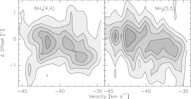
Figure 2.— G305.21+0.21 position velocity diagrams of the main hyperfine components of NH₃(4,4) (left) and NH₃(5,5) (right). The diagrams are centered at Offsets $(0^{\prime\prime}/0^{\prime\prime})$ with a position angle of -45 degrees from north (northwest-southeast direction).

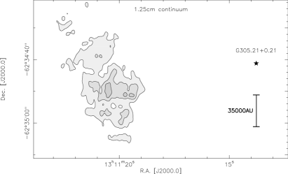
Figure 3.— 1.25 cm continuum emission in the field of G305.21+0.21. The contour levels are in $3\sigma$ steps (Table 2). The star marks the position of our primary NH₃ target within the field, and a scale-bar is shown at the bottom-right.

Figure 4.— G316.81-0.06 intensity weighted velocity (1st moment, top row) and line width (2nd moment, bottom row) maps of the main hyperfine components of NH₃(4,4) (left) and NH₃(5,5) (right). The triangles mark the Class II CH₃OH maser positions (Walsh et al., 1998), and the synthesized beams are shown at the bottom-left of each panel, a scale-bar is presented in the top-left panel, and the 0/0 position is given in Table 1.

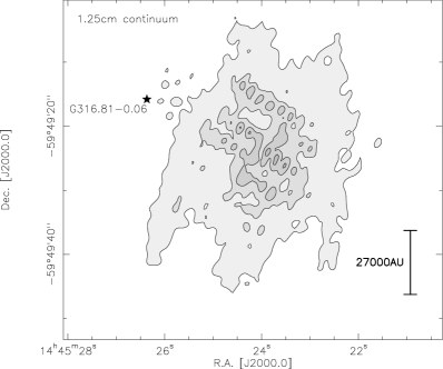
Figure 5.— 1.25 cm continuum emission in the field of G316.81-0.06. The contours start at the $5\sigma$ level and continue in $3\sigma$ steps (Table 2). The star marks the position of our primary NH₃ target within the field, and a scale-bar is shown at the bottom-right.

Figure 6.— G323.74-0.26 intensity weighted velocity (1st moment, top row) and line width (2nd moment, bottom row) maps of the main hyperfine components of NH₃(4,4) (left) and NH₃(5,5) (right). The triangles mark the Class II CH₃OH maser positions (Walsh et al., 1998), the synthesized beams are shown at the bottom-left of each panel, a scale-bar is presented in the top-left panel, and the 0/0 position is given in Table 1.

Figure 7.— G327.3-0.60 intensity weighted velocity (1st moment) maps of the main hyperfine components of NH₃(4,4) (left) and NH₃(5,5) (right) excluding antenna 6 to better show the larger-scale structure. The triangles mark the positions of the Class II CH₃OH masers (James Caswell, private communication as referred to by Caswell 1998), the synthesized beams are shown at the bottom-right of each panel, a scale-bar assuming near kinematic distance is presented in the left panel, and the 0/0 position is given in Table 1.

Figure 8.— G327.3-0.60 intensity weighted velocity (1st moment, top row) and line width (2nd moment, bottom row) maps of the main hyperfine components of NH₃(4,4) (left) and NH₃(5,5) (middle) including also antenna 6 data to also show the smaller-scale sub-structure. The right panel shows the 1st moment map of the most blue-shifted NH₃(4,4) hyperfine component. The triangles mark the positions of the Class II CH₃OH masers (James Caswell, private communication as referred to by Caswell 1998), the synthesized beams are shown at the bottom-left of each panel, a scale-bar assuming near kinematic distance is presented in the bottom-left panel, and the 0/0 position is given in Table 1.

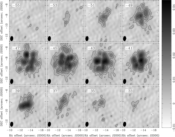
Figure 9.— Channel map of the main hyperfine component of NH₃(4,4) with a spectral resolution of 2 km s^-1 in G327.3-0.60. The contour levels (positive full lines, negative dashed lines) are in $3\sigma$ steps with a $1\sigma$ value of 1.6 mJy beam^-1. The synthesized beams are shown at the bottom-left of each panel, and the 0/0 position is given in Table 1.

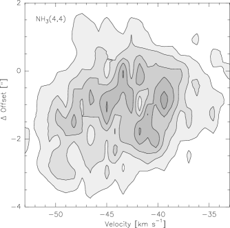
Figure 10.— G327.3-0.60 position velocity diagram of the main hyperfine components of NH₃(4,4) (left). The diagram is centered at offset $(-12.5^{\prime\prime}/-9.1^{\prime\prime})$ with a position angle of 140 degrees from north (northwest-southeast direction).

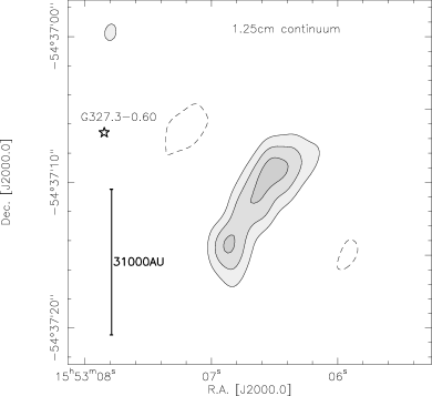
Figure 11.— 1.25 cm continuum emission in the field of G327.3-0.60. The contour levels start at $3\sigma$ and continue in $2\sigma$ steps (Table 2, full lines positive, and dashed lines negative features). The star marks the position of our primary NH₃ target within the field, and a scale-bar is shown at the bottom-right.

Figure 12.— G328.81+0.63: The grey-scales present the 1st moment maps of the absorption features of the main NH₃(4,4) and (5,5) hyperfine components (top and bottom panels, respectively) against the ultracompact Hii region outlined in contours from the 1.25 cm continuum emission. The contouring is done in $6\sigma$ steps of 16.8 mJy beam^-1. The triangles mark the Class II CH₃OH maser positions (Walsh et al., 1998), and the synthesized beams and scale-bars are plotted at the bottom left of each panel.

Figure 13.— G328.81+0.63 centered on the brightest eastern peak from Figure 12: The grey-scale presents the 1st moment maps of the absorption features of the main NH₃(4,4) hyperfine component against the ultracompact Hii region outlined in contours from the 1.25 cm continuum emission. The contouring is done in $6\sigma$ steps of 16.8 mJy beam^-1.

Figure 14.— G328.81+0.63: The grey-scales present the 2nd moment maps of the absorption features of the main NH₃(4,4) hyperfine component against the ultracompact Hii region outlined in contours from the 1.25 cm continuum emission. The contouring is done in $6\sigma$ steps of 16.8 mJy beam^-1. The triangles mark the Class II CH₃OH maser positions (Walsh et al., 1998), and the synthesized beam and scale-bar are plotted at the bottom left of each panel.

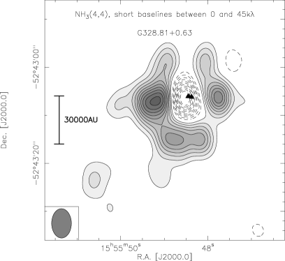
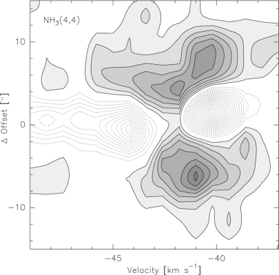
Figure 15.— G328.81+0.63: Top: Integrated NH₃(4,4) emission from -47.5 to -37.5 km s^-1. To produce this map, we only used the short baselines between 0 and 45 $k\lambda$. The contouring is done in $\pm 3\sigma$ steps of 2.7 mJy beam^-1. The triangles mark the Class II CH₃OH maser positions, the synthesized beam and the scale-bar are plotted at the left. Bottom: The corresponding position-velocity diagram through the center in east-west direction. The contouring is done in $3\sigma$ levels of 6.6 mJy beam, measured in an 0.8 km s${}^{{}_{1}}$ channel. Full lines show emission, dotted lines absorption.

Figure 16.— G331.28-0.19 intensity weighted velocity (1st moment, top row) and line width (bottom row) maps of the main hyperfine components of NH₃(4,4) (left) and NH₃(5,5) (right). The contours show the 1.25 cm continuum emission with contour levels in $3\sigma$ steps of 0.9 mJy beam^-1. The white triangles mark the Class II CH₃OH maser positions (Walsh et al., 1998), the arrows in the top-left panel outline the approximate direction of the outflow (Table 1), the synthesized beams are shown at the bottom-left of each panel, a scale-bar is presented in the top-left panel, and the 0/0 position is given in Table 1.

Figure 17.— G336.02-0.83 intensity weighted velocity (1st moment, top row) and line width (2nd moment, bottom row) maps of the main hyperfine components of NH₃(4,4) and NH₃(5,5) excluding the long baselines associated with antenna 6. The triangles mark the Class II CH₃OH maser positions by Walsh et al. (1998), the synthesized beams are shown at the bottom-left of each panel, a scale-bar adopting the near kinematic distance is presented in the top-left panel, and the 0/0 position is given in Table 1.

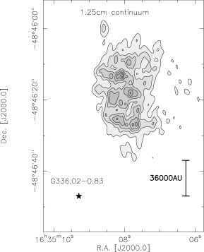
Figure 18.— 1.25 cm continuum emission in the field of G336.02-0.83. The contour levels are at $3\sigma$ intervals (Table 2). The star marks the position of our primary NH₃ target within the field, and a scale-bar adopting the near kinematic distance is presented in the bottom-right.

Figure 19.— G345.00-0.22 intensity weighted velocity maps (1st moment) of the main hyperfine components of NH₃(4,4) and (5,5) in the left and right panels, respectively. The contours show the 1.25 cm continuum emission starting at the $4\sigma$ level and continuing in $6\sigma$ steps. While the main panels show the NH₃ in emission, the inset presents the absorption against the continuum. The triangles mark the Class II CH₃OH maser positions by Walsh et al. (1998), the synthesized beams are shown at the bottom-left of the two bottom panels, a scale-bar adopting the near kinematic distance is presented in the top-left panel, and the 0/0 position is given in Table 1.

Figure 20.— G345.00-0.22 intensity line width maps (2nd moment) of the main hyperfine components of NH₃(4,4) and (5,5) in the left and right panels, respectively. The contours show the 1.25 cm continuum emission starting at the $4\sigma$ level and continuing in $6\sigma$ steps. The triangles mark the Class II CH₃OH maser positions by Walsh et al. (1998), the synthesized beams are shown at the bottom-left of the two bottom panels, a scale-bar adopting the near kinematic distance is presented in the top-left panel, and the 0/0 position is given in Table 1.

Figure 21.— G351.77-0.54 intensity weighted velocity (1st moment) maps of the main hyperfine components of NH₃(4,4) (left) and NH₃(5,5) (right). The triangles mark the positions of the Class II CH₃OH masers (Walsh et al., 1998), the arrows and stars in the left panel outline the approximate direction of the outflow (Table 1) and the positions of the cm sources from Zapata et al. (2008). The synthesized beams are shown at the bottom-left, a scale-bar is presented in the bottom-left panel, and the 0/0 position is given in Table 1.

Figure 22.— G351.77-0.54 intensity weighted velocity (1st moment, top row) and line width (2nd moment, bottom row) maps of the main hyperfine components of NH₃(4,4) (left) and NH₃(5,5) (right). The triangles mark the positions of the Class II CH₃OH masers (Walsh et al., 1998), the arrows and stars in the top-left panel outline the approximate direction of the outflow (Table 1) and the positions of the cm sources from Zapata et al. (2008). The synthesized beams are shown at the bottom-left of each panel, a scale-bar is presented in the top-left panel, and the 0/0 position is given in Table 1.

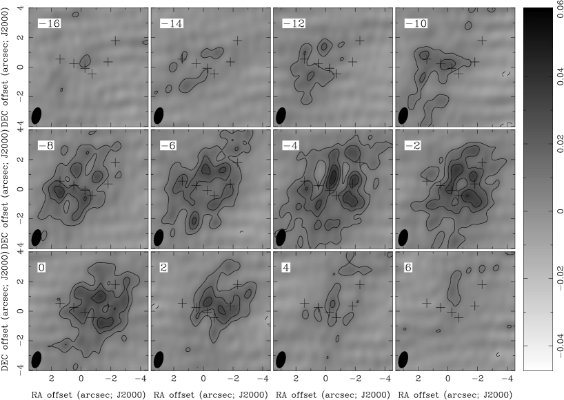
Figure 23.— Channel map of the main hyperfine component of NH₃(4,4) with a spectral resolution of 2 km s^-1 in G351.77-0.54 . The contour levels (positive full lines, negative dashed lines) are in $3\sigma$ steps with a $1\sigma$ value of 3.3 mJy beam^-1. The crosses mark the cm continuum sources from Zapata et al. (2008), and the synthesized beams are shown at the bottom-left of each panel, and the 0/0 position is given in Table 1.

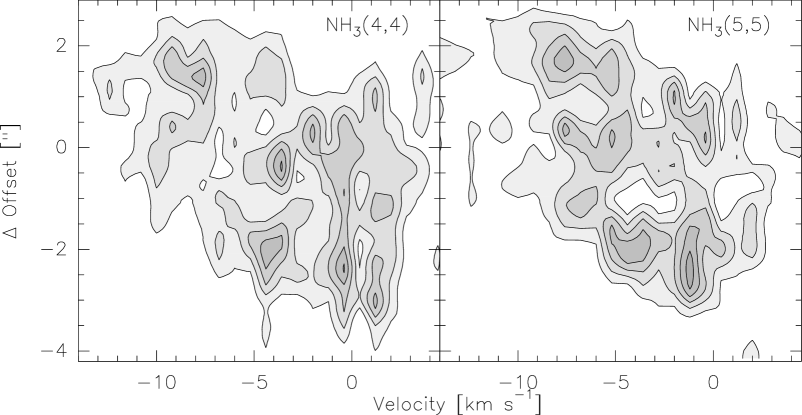
Figure 24.— G351.77-0.54 position velocity diagrams of the main hyperfine components of NH₃(4,4) (left) and NH₃(5,5) (right). The diagrams are centered at Offsets $(0^{\prime\prime}/0^{\prime\prime})$ with a position angle of 105 degrees from north (ESE-WNW).

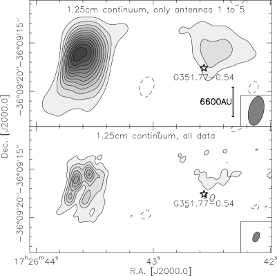
Figure 25.— 1.25 cm continuum emission in the field of G351.77-0.54. The top-panel shows the data excluding the long baselines associated with antenna 6, hence with lower spatial resolution (Table 2). The contour levels are in $3\sigma$ steps (Table 2, full lines positive, and dashed lines negative features). The star marks the position of our primary NH₃ target within the field, and a scale-bar is presented in the top panel.

Figure 26.— G0.55-0.85 intensity weighted velocity (1st moment, top row) and line width (2nd moment, bottom row) maps of the main hyperfine components of NH₃(4,4) and (5,5). The triangles mark the Class II CH₃OH maser positions by Walsh et al. (1998), the synthesized beams are shown at the bottom-right of each panel, a scale-bar adopting the near kinematic distance is presented in the top-left panel, and the 0/0 position is given in Table 1.

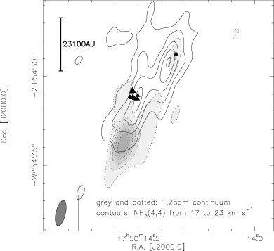
Figure 27.— The grey-scale with dotted contours shows the 1.25 cm continuum emission in the field of G0.55-0.85. The contour levels are at $3\sigma$ intervals (Table 2). The full contours present the NH₃(4,4) emission integrated from 13 to 21 km s^-1 with contour levels at $3\sigma$ steps of 4.8 mJy beam^-1. The triangles mark the Class II CH₃OH maser positions by Walsh et al. (1998), the synthesized beam of the continuum data is shown at the bottom left, and a scale-bar adopting the near kinematic distance is presented in the top-left.

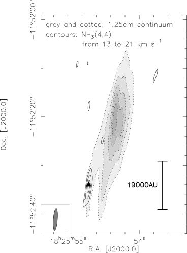
Figure 28.— The grey-scale with dotted contours shows the 1.25 cm continuum emission in the field of G19.47+0.17. The contour levels are at $3\sigma$ intervals (Table 2). The full contours present the NH₃(4,4) emission integrated from 17 to 23 km s^-1 with contour levels starting at the $4\sigma$ level of 5.6 mJy beam^-1 and continuing at $3\sigma$ steps. The triangles mark the Class II CH₃OH maser positions (Walsh et al., 1998), the synthesized beam of the NH₃ data is shown at the bottom left, and a scale-bar is presented in the bottom-right.

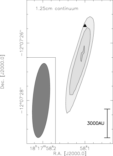
Figure 29.— 1.25 cm continuum emission in the field of IRAS 18151-1208. The contour levels start at the $3\sigma$ level and continue in $1\sigma$ steps (Table 2). The triangle marks the Class II CH₃OH maser position from Beuther et al. (2002c), the synthesized beam is shown at the bottom left, and a scale-bar is presented in the bottom-right.

Figure 30.— NH₃(4,4) and NH₃(5,5) spectra (left and right column) extracted toward the peak positions of the sources labeled in each panel. The histogram presents the data whereas the full lines show attempts to fit the whole hyperfine structure. Due to the very high optical depth, even this hyperfine structure fitting does not work well.

Figure 31.— NH₃(4,4) and NH₃(5,5) spectra (left and right column) extracted toward the peak positions of the sources labeled in each panel. For G328.81+0.63, the shown spectrum is extracted toward the large-scale western peak in Figure 15. The histogram presents the data whereas the full lines show attempts to fit the whole hyperfine structure. Due to the very high optical depth, even this hyperfine structure fitting does not work well.

Figure 32.— NH₃(4,4) and NH₃(5,5) spectra (left and right column) extracted toward the peak positions of the sources labeled in each panel. The histogram presents the data whereas the full lines show attempts to fit the whole hyperfine structure. Due to the very high optical depth, even this hyperfine structure fitting does not work well (it did not work at all for the (4,4) line of G351.77-0.54).

References

- Araya et al. (2007) Araya, E., Hofner, P., Sewiło, M., et al. 2007, ApJ, 669, 1050
- Arce et al. (2007) Arce, H. G., Shepherd, D., Gueth, F., et al. 2007, in Protostars and Planets V, ed. B. Reipurth, D. Jewitt, & K. Keil, 245–260
- Bally & Zinnecker (2005) Bally, J. & Zinnecker, H. 2005, AJ, 129, 2281
- Beuther et al. (2007a) Beuther, H., Churchwell, E. B., McKee, C. F., & Tan, J. C. 2007a, in Protostars and Planets V, ed. B. Reipurth, D. Jewitt, & K. Keil, 165–180
- Beuther et al. (2002a) Beuther, H., Schilke, P., Gueth, F., et al. 2002a, A&A, 387, 931
- Beuther et al. (2002b) Beuther, H., Schilke, P., Sridharan, T. K., et al. 2002b, A&A, 383, 892
- Beuther & Shepherd (2005) Beuther, H. & Shepherd, D. 2005, in Cores to Clusters: Star Formation with Next Generation Telescopes, ed. M. S. N. Kumar, M. Tafalla, & P. Caselli, 105–119
- Beuther et al. (2005) Beuther, H., Thorwirth, S., Zhang, Q., et al. 2005, ApJ, 627, 834
- Beuther et al. (2002c) Beuther, H., Walsh, A., Schilke, P., et al. 2002c, A&A, 390, 289
- Beuther & Walsh (2008) Beuther, H. & Walsh, A. J. 2008, ApJ, 673, L55
- Beuther et al. (2007b) Beuther, H., Walsh, A. J., Thorwirth, S., et al. 2007b, A&A, 466, 989
- Beuther et al. (2009) Beuther, H., Zhang, Q., Bergin, E. A., & Sridharan, T. K. 2009, AJ, 137, 406
- Bonnell et al. (2007) Bonnell, I. A., Larson, R. B., & Zinnecker, H. 2007, in Protostars and Planets V, ed. B. Reipurth, D. Jewitt, & K. Keil, 149–164
- Bonnell et al. (2004) Bonnell, I. A., Vine, S. G., & Bate, M. R. 2004, MNRAS, 349, 735
- Brand & Blitz (1993) Brand, J. & Blitz, L. 1993, A&A, 275, 67
- Caswell (1998) Caswell, J. L. 1998, MNRAS, 297, 215
- Caswell et al. (1995) Caswell, J. L., Vaile, R. A., Ellingsen, S. P., Whiteoak, J. B., & Norris, R. P. 1995, MNRAS, 272, 96
- Cesaroni et al. (2007) Cesaroni, R., Galli, D., Lodato, G., Walmsley, C. M., & Zhang, Q. 2007, in Protostars and Planets V, ed. B. Reipurth, D. Jewitt, & K. Keil, 197–212
- Chini et al. (2004) Chini, R., Hoffmeister, V., Kimeswenger, S., et al. 2004, Nature, 429, 155
- Davis et al. (2004) Davis, C. J., Varricatt, W. P., Todd, S. P., & Ramsay Howat, S. K. 2004, A&A, 425, 981
- De Buizer (2003) De Buizer, J. M. 2003, MNRAS, 341, 277
- De Buizer et al. (2008) De Buizer, J. M., Redman, R. O., Longmore, S. N., Caswell, J., & Feldman, P. A. 2008, ArXiv e-prints
- Fish et al. (2005) Fish, V. L., Reid, M. J., Argon, A. L., & Zheng, X.-W. 2005, ApJS, 160, 220
- Forster et al. (1990) Forster, J. R., Caswell, J. L., Okumura, S. K., Ishiguro, M., & Hasegawa, T. 1990, A&A, 231, 473
- Jijina & Adams (1996) Jijina, J. & Adams, F. C. 1996, ApJ, 462, 874
- Kahn (1974) Kahn, F. D. 1974, A&A, 37, 149
- Keto (2002) Keto, E. 2002, ApJ, 568, 754
- Keto (2003) Keto, E. 2003, ApJ, 599, 1196
- Keto (2007) Keto, E. 2007, ApJ, 666, 976
- Kratter & Matzner (2006) Kratter, K. M. & Matzner, C. D. 2006, MNRAS, 373, 1563
- Krumholz et al. (2007a) Krumholz, M. R., Klein, R. I., & McKee, C. F. 2007a, ApJ, 665, 478
- Krumholz et al. (2007b) Krumholz, M. R., Klein, R. I., & McKee, C. F. 2007b, ApJ, 656, 959
- Krumholz et al. (2009) Krumholz, M. R., Klein, R. I., McKee, C. F., Offner, S. S. R., & Cunningham, A. J. 2009, Science, 323, 754
- Leurini et al. (2008) Leurini, S., Hieret, C., Thorwirth, S., et al. 2008, A&A, 485, 167
- Longmore & Burton (2009) Longmore, S. N. & Burton, M. G. 2009, ArXiv e-prints, 0906.3353
- Longmore et al. (2007a) Longmore, S. N., Burton, M. G., Barnes, P. J., et al. 2007a, MNRAS, 379, 535
- Longmore et al. (2009) Longmore, S. N., Burton, M. G., Keto, E., Kurtz, S., & Walsh, A. J. 2009, MNRAS, 1151
- Longmore et al. (2007b) Longmore, S. N., Maercker, M., Ramstedt, S., & Burton, M. G. 2007b, MNRAS, 380, 1497
- McKee & Tan (2003) McKee, C. F. & Tan, J. C. 2003, ApJ, 585, 850
- Noriega-Crespo et al. (2004) Noriega-Crespo, A., Morris, P., Marleau, F. R., et al. 2004, ApJS, 154, 352
- Norris et al. (1993) Norris, R. P., Whiteoak, J. B., Caswell, J. L., Wieringa, M. H., & Gough, R. G. 1993, ApJ, 412, 222
- Osorio et al. (2009) Osorio, M., Anglada, G., Lizano, S., & D’Alessio, P. 2009, ApJ, 694, 29
- Purcell et al. (2006) Purcell, C. R., Balasubramanyam, R., Burton, M. G., et al. 2006, MNRAS, 367, 553
- Purcell et al. (2009) Purcell, C. R., Longmore, S. N., Burton, M. G., et al. 2009, MNRAS, 394, 323
- Simon et al. (2000) Simon, M., Dutrey, A., & Guilloteau, S. 2000, ApJ, 545, 1034
- Sollins et al. (2005) Sollins, P. K., Zhang, Q., Keto, E., & Ho, P. T. P. 2005, ApJ, 624, L49
- Sridharan et al. (2002) Sridharan, T. K., Beuther, H., Schilke, P., Menten, K. M., & Wyrowski, F. 2002, ApJ, 566, 931
- Vaidya et al. (2009) Vaidya, B., Fendt, C., & Beuther, H. 2009, ApJ, 702, 567
- Walmsley & Ungerechts (1983) Walmsley, C. M. & Ungerechts, H. 1983, A&A, 122, 164
- Walsh et al. (1998) Walsh, A. J., Burton, M. G., Hyland, A. R., & Robinson, G. 1998, MNRAS, 301, 640
- Walsh et al. (2002) Walsh, A. J., Lee, J.-K., & Burton, M. G. 2002, MNRAS, 329, 475
- Wolfire & Cassinelli (1987) Wolfire, M. G. & Cassinelli, J. P. 1987, ApJ, 319, 850
- Yorke & Sonnhalter (2002) Yorke, H. W. & Sonnhalter, C. 2002, ApJ, 569, 846
- Zapata et al. (2005) Zapata, L., Rodriguez, L., Ho, P., Beuther, H., & Zhang, Q. 2005, ArXiv Astrophysics e-prints
- Zapata et al. (2008) Zapata, L. A., Leurini, S., Menten, K. M., et al. 2008, AJ, 136, 1455
- Zhang (2005) Zhang, Q. 2005, in IAU Symposium, Vol. 227, Massive Star Birth: A Crossroads of Astrophysics, ed. R. Cesaroni, M. Felli, E. Churchwell, & M. Walmsley, 135–144
- Zhang et al. (1998) Zhang, Q., Hunter, T. R., & Sridharan, T. K. 1998, ApJ, 505, L151
- Zinnecker & Yorke (2007) Zinnecker, H. & Yorke, H. W. 2007, ARA&A, 45, 481