Relative $(p,{\varepsilon})$-Approximations in Geometry

Abstract

We re-examine the notion of relative $(p,{\varepsilon})$-approximations, recently introduced in [CKMS06], and establish upper bounds on their size, in general range spaces of finite VC-dimension, using the sampling theory developed in [LLS01] and in several earlier studies [Pol86, Hau92, Tal94]. We also survey the different notions of sampling, used in computational geometry, learning, and other areas, and show how they relate to each other. We then give constructions of smaller-size relative $(p,{\varepsilon})$-approximations for range spaces that involve points and halfspaces in two and higher dimensions. The planar construction is based on a new structure—spanning trees with small relative crossing number, which we believe to be of independent interest. Relative $(p,{\varepsilon})$-approximations arise in several geometric problems, such as approximate range counting, and we apply our new structures to obtain efficient solutions for approximate range counting in three dimensions. We also present a simple solution for the planar case.

1 Introduction

The main problem that has motivated the study in this paper is approximate range counting. In a typical example, one is given a set $P$ of points in the plane, and the goal is to preprocess $P$ into a data structure which supports efficient approximate counting of the number of points of $P$ that lie inside a query halfplane. The hope is that approximate counting can be done more efficiently than exact counting.

This is an instance of a more general and abstract setting. In general, we are given a range space $(X,\mathcal{R})$, where $X$ is a set of $n$ objects and $\mathcal{R}$ is a collection of subsets of $X$, called ranges. In a typical geometric setting, $X$ is a subset of some infinite ground set $U$ (e.g., $U={\mathbb{R}}^{d}$ and $X$ is a finite point set in ${\mathbb{R}}^{d}$), and $\mathcal{R}=\left\{{\mathfrak{r}\cap X\,\left|\,{\mathfrak{r}\in\mathcal{R}_{U}}\rule[-5.69046pt]{0.0pt}{11.38092pt}\right.}\right\}$, where $\mathcal{R}_{U}$ is a collection of subsets (ranges) of $U$ of some simple shape, such as halfspaces, simplices, balls, etc. (To simplify the notation, we will use $\mathcal{R}$ and $\mathcal{R}_{U}$ interchangeably.) The measure of a range $\mathfrak{r}\in\mathcal{R}$ in $X$ is the quantity

$$\overline{X}\!\left({\mathfrak{r}}\right)=\frac{\left|{X\cap\mathfrak{r}}\right|}{\left|{X}\right|}.$$

Given $(X,\mathcal{R})$ as above, and a parameter $0<{\varepsilon}<1$, the goal is to preprocess $X$ into a data structure that supports efficient queries of the form: Given $\mathfrak{r}\in\mathcal{R}_{U}$, compute a number $t$ such that

$$(1-{\varepsilon})\overline{X}\!\left({\mathfrak{r}}\right)\leq t\leq(1+{\varepsilon})\overline{X}\!\left({\mathfrak{r}}\right).$$ (1)

We refer to the estimate $t\left|{X}\right|$ as an ${\varepsilon}$-approximate count of $X\cap\mathfrak{r}$.

The motivation for seeking approximate range counting techniques is that exact range counting (i.e., computing the exact value $\overline{X}\!\left({\mathfrak{r}}\right)$, for $\mathfrak{r}\in\mathcal{R}$) is (more) expensive. For instance, consider the classical halfspace range counting problem [Mat92], which is the main application considered in this paper. Here, for a set $P$ of $n$ points in ${\mathbb{R}}^{d}$, for $d\geq 2$, the best known algorithm for exact halfspace range counting with near-linear storage takes $O(n^{1-1/d})$ time [Mat92]. As shown in several recent papers, if we only want to approximate the count, as in Eq. (1), there exist faster solutions, in which the query time is close to $O(n^{1-1/\lfloor d/2\rfloor})$ (and is polylogarithmic in two and three dimensions) [AH08, AS08, KS06, KRS08a, KRS08b].

Notice that the problem of approximate range counting becomes more challenging as the size of $X\cap\mathfrak{r}$ decreases. At the extreme, when $\left|{X\cap\mathfrak{r}}\right|<1/{\varepsilon}$, we must produce the count exactly. In particular, we need to be able to detect (without any error) whether a given query range $\mathfrak{r}$ is empty, i.e., satisfies $X\cap\mathfrak{r}=\emptyset$. Thus, approximate range counting (in the sense defined above) is at least as hard as range emptiness detection.

We make the standard assumption that the range space $(X,\mathcal{R})$ (or, in fact, $(U,\mathcal{R}_{U})$) has finite VC-dimension $\delta$, which is a constant independent of $n$. This is indeed the case in many geometric applications. In general, range spaces involving semi-algebraic ranges of constant description complexity, i.e., semi-algebraic sets defined as a Boolean combination of a constant number of polynomial equations and inequalities of constant maximum degree, have finite VC-dimension. Halfspaces, balls, ellipsoids, simplices, and boxes are examples of ranges of this kind; see [Cha01, HW87, Mat99, PA95] for definitions and more details.

Known notions of approximations.

A standard and general technique for tackling the approximate range counting problem is to use ${\varepsilon}$-approximations. An (absolute-error) ${\varepsilon}$-approximation for $(X,\mathcal{R})$ is a subset $Z\subset X$ such that, for each $\mathfrak{r}\in\mathcal{R}$, $\left|{\overline{Z}\!\left({\mathfrak{r}}\right)-\overline{X}\!\left({\mathfrak{r}}\right)}\right|<{\varepsilon}$. In the general case, it is known that a random sample of size $O\left(\frac{\delta}{{\varepsilon}^{2}}\right)$ is an ${\varepsilon}$-approximation with at least some positive constant probability [LLS01, Tal94], and improved bounds are known in certain special cases; see below for details.

Another notion of approximation was introduced by Brönnimann et al. [Brö95, BCM99]. A subset $Z\subseteq X$ is a sensitive ${\varepsilon}$-approximation if for all ranges $\mathfrak{r}\in\mathcal{R}$, we have $\left|{\overline{X}\!\left({\mathfrak{r}}\right)-\overline{Z}\!\left({\mathfrak{r}}\right)}\right|\leq({\varepsilon}/2)\!\left({\overline{X}\!\left({\mathfrak{r}}\right)^{1/2}+{\varepsilon}}\right)$. Brönnimann et al. present a deterministic algorithm for computing sensitive approximations of size $O\!\left({\frac{\delta}{{\varepsilon}^{2}}{\log\frac{\delta}{{\varepsilon}}}}\right)$, in deterministic time $O(\delta)^{3\delta}(1/{\varepsilon})^{2\delta}\log^{\delta}(\delta/{\varepsilon})|X|$.

Another interesting notion of sampling, studied by Li et al. [LLS01], is a $(\nu,\alpha)$-sample. For given parameters $\alpha,\nu>0$, a sample $Z\subseteq X$ is a $(\nu,\alpha)$-sample if, for any range $\mathfrak{r}\in\mathcal{R}$, we have $d_{\nu}(\overline{Z}\!\left({\mathfrak{r}}\right),\overline{X}\!\left({\mathfrak{r}}\right))\leq\alpha$, where $d_{\nu}(x,y)=\left|{x-y}\right|/(x+y+\nu)$. Li et al. gave the currently best known upper bound on the size of a sample which guarantees this property, showing that a random sample of $X$ of size $O\!\left({\frac{1}{\alpha^{2}\nu}\left(\delta\log\frac{1}{\nu}+\log\frac{1}{q}\right)}\right)$ is a $(\nu,\alpha)$-sample with probability at least $1-q$; see below for more details.

Relative $(p,{\varepsilon})$-approximation.

In this paper, we consider a variant of these classical structures, originally proposed a few years ago by Cohen et al. [CKMS06], which provides relative-error approximations. Ideally, we want a subset $Z\subset X$ such that, for each $\mathfrak{r}\in\mathcal{R}$, we have

$$(1-{\varepsilon})\overline{X}\!\left({\mathfrak{r}}\right)\leq\overline{Z}\!\left({\mathfrak{r}}\right)\leq(1+{\varepsilon})\overline{X}\!\left({\mathfrak{r}}\right).$$ (2)

This “definition” suffers however from the same syndrome as approximate range counting; that is, as $\left|{X\cap\mathfrak{r}}\right|$ shrinks, the absolute precision of the approximation has to increase. At the extreme, when $Z\cap\mathfrak{r}=\emptyset$, $X\cap\mathfrak{r}$ must also be empty; in general, we cannot guarantee this property, unless we take $Z=X$, which defeats the purpose of using small-size ${\varepsilon}$-approximations to speed up approximate counting.

For this reason, we refine the definition, introducing another fixed parameter $0<p<1$. We say that a subset $Z\subset X$ is a relative $(p,{\varepsilon})$-approximation if it satisfies Eq. (2) for each $\mathfrak{r}\in\mathcal{R}$ with $\overline{X}\!\left({\mathfrak{r}}\right)\geq p$. For smaller ranges $\mathfrak{r}$, the error term ${\varepsilon}\overline{X}\!\left({\mathfrak{r}}\right)$ in Eq. (2) is replaced by ${\varepsilon}p$. As we will shortly observe, relative $(p,{\varepsilon})$-approximations are equivalent to $(\nu,\alpha)$-samplings, with appropriate relations between $p$, ${\varepsilon}$, and $\nu$, $\alpha$ (see Theorem 2.9), but this new notion provides a better working definition for approximate range counting and for other applications.

Known results.

As shown by Vapnik and Chervonenkis [VC71] (see also [Cha01, Mat99, PA95]), there always exist absolute-error ${\varepsilon}$-approximations of size $\frac{c\delta}{{\varepsilon}^{2}}\log\frac{\delta}{{\varepsilon}}$, where $c$ is an absolute constant. Moreover, a random sample of this size from $X$ is an ${\varepsilon}$-approximation with constant positive probability. This bound has been strengthened by Li et al. [LLS01] (see also [Tal94]), who have shown that a random sample of size $\frac{c}{{\varepsilon}^{2}}\left(\delta+\log\frac{1}{q}\right)$ is an ${\varepsilon}$-approximation with probability at least $1-q$, for a sufficiently large (absolute) constant $c$. (Interestingly, until very recently, this result, worked out in the context of machine learning applications, does not seem to have been known within the computational geometry literature.) ${\varepsilon}$-approximations of size $O\!\left({\frac{\delta}{{\varepsilon}^{2}}\log\frac{\delta}{{\varepsilon}}}\right)$ can also be constructed in deterministic time $O\left(\delta^{3\delta}\left(\frac{1}{{\varepsilon}^{2}}\log\frac{\delta}{{\varepsilon}}\right)^{\delta}n\right)$ [Cha04].

As shown in [Cha01, Cha04, MWW93], there always exist smaller (absolute-error) ${\varepsilon}$-approximations, of size

$$O\!\left({\frac{1}{{\varepsilon}^{2-2/(\delta^{\prime}+1)}}\log^{b-b/(\delta^{\prime}+1)}\frac{1}{{\varepsilon}}}\right),$$

where $\delta^{\prime}$ is the exponent of either the primal shatter function of the range space $(X,\mathcal{R})$ (and then $b=2$) or the dual shatter function (and then $b=1$). The time to construct these improved ${\varepsilon}$-approximations is roughly the same as the deterministic time bound of [Cha04] stated above, for the case of the dual shatter function. For the case of the primal shatter function, the proof is only existential.

Consider next relative $(p,{\varepsilon})$-approximations. One of the contributions of this paper is to show that these approximations are in fact just an equivalent variant of the $(\nu,\alpha)$-samplings of Li et al. [LLS01]; see Section 2. As a consequence, the analysis of [LLS01] implies that there exist relative $(p,{\varepsilon})$-approximations of size $\frac{c\delta}{{\varepsilon}^{2}p}\log\frac{1}{p}$, where $c$ is an absolute constant. In fact, any random sample of these many elements of $X$ is a relative $(p,{\varepsilon})$-approximation with constant probability. Success with probability at least $1-q$ is guaranteed if one samples $\frac{c}{{\varepsilon}^{2}p}\!\left({\delta\log\frac{1}{p}+\log\frac{1}{q}}\right)$ elements of $X$, for a sufficiently large constant $c$ [LLS01].

To appreciate the above bound on the size of relative $(p,{\varepsilon})$-approximations, it is instructive to observe that, for a given parameter $p$, any absolute error $({\varepsilon}p)$-approximation $Z$ will approximate “large” ranges (of measure at least $p$) to within relative error ${\varepsilon}$, as in Eq. (2), as is easily checked (and the inequality for smaller ranges is also trivially satisfied), so $Z$ is a relative $(p,{\varepsilon})$-approximation. However, the Vapnik-Chervonenkis bound on the size of $Z$, namely, $\frac{c\delta}{{\varepsilon}^{2}p^{2}}\log\frac{\delta}{{\varepsilon}p}$, as well as the improved bound of [LLS01, Tal94], are larger by roughly a factor of $1/p$ than the improved bound stated above.

The existence of a relative $(p,{\varepsilon})$-approximation $Z$ provides a simple mechanism for approximate range counting: Given a range $\mathfrak{r}\in\mathcal{R}$, count $Z\cap\mathfrak{r}$ exactly, say, by brute force in $O(\left|{Z}\right|)$ time, and output $\left|{Z\cap\mathfrak{r}}\right|\cdot\left|{X}\right|/\left|{Z}\right|$ as a (relative) ${\varepsilon}$-approximate count of $X\cap\mathfrak{r}$. However, this will work only for ranges of size at least $pn$. Aronov and Sharir [AS08] show that an appropriate incorporation of relative $(p,{\varepsilon})$-approximations into standard range searching data structures yields a procedure for approximate range counting that works, quite efficiently, for ranges of any size. This has recently been extended, by Sharir and Shaul [SS09], to approximate range counting with general semi-algebraic ranges.

Our results.

In this paper, we present several constructions and bounds involving relative $(p,{\varepsilon})$-approximations.

We first consider samplings in general range spaces of finite VC-dimension, and establish relations between several different notions of samplings, including $(\nu,\alpha)$-samplings, relative $(p,{\varepsilon})$-approximations, and sensitive ${\varepsilon}$-approximations. Our main observations are:

(i) The notion of $(p,{\varepsilon})$-approximation is equivalent to that of $(\nu,\alpha)$-sample, by choosing $\nu$ to be proportional to $p$ and $\alpha$ proportional to ${\varepsilon}$; see Theorem 2.9.

(ii) A sensitive $({\varepsilon}\sqrt{p})$-approximation is also a relative $(p,{\varepsilon})$-approximation.

(iii) The result of Li et al. [LLS01] is sufficiently powerful, so as to imply known bounds on the size of many of the different notions of samplings, including ${\varepsilon}$-nets, ${\varepsilon}$-approximations, sensitive ${\varepsilon}$-approximations, and, as just said, relative $(p,{\varepsilon})$-approximations. Some of these connections have already been noted earlier, in [LLS01] and in [Har08]. We offer this portion of Section 2 as a service to the computational geometry community, which, as already noted, is not as aware of the results of [LLS01] and of their implications as the machine learning community.

Next, we return to geometric range spaces, and study two cases where one can construct relative $(p,{\varepsilon})$-approximations of smaller size. The first case involves planar point sets and halfplane ranges, and the second case involves point sets in ${\mathbb{R}}^{d}$, $d\geq 3$, and halfspace ranges. In the planar case, we show the existence, and provide efficient algorithms for the construction, of relative $(p,{\varepsilon})$-approximations of size $O\!\left({\frac{1}{{\varepsilon}^{4/3}p}\log\frac{1}{{\varepsilon}p}}\right)$. Our technique also shows in this case the existence of sensitive ${\varepsilon}$-approximations with improved quality of approximation. Specifically, for a planar point set $X$, we show that there exists a subset $Z\subseteq X$ of size $O\!\left({\frac{1}{{\varepsilon}^{2}}\log^{4/3}\frac{1}{{\varepsilon}}}\right)$, such that, for any halfplane $\mathfrak{r}$, we have $\left|{\overline{X}\!\left({\mathfrak{r}}\right)-\overline{Z}\!\left({\mathfrak{r}}\right)}\right|\leq\frac{1}{2}{\varepsilon}^{3/2}\overline{X}\!\left({\mathfrak{r}}\right)^{1/4}+{\varepsilon}^{2}$. (This new error term is indeed an improvement when $\overline{X}\!\left({\mathfrak{r}}\right)>{\varepsilon}^{2}$ and is the same as the standard term otherwise.)

In the planar case, the construction is based on an interesting generalization of spanning trees with small crossing number, a result that we believe to be of independent interest. Specifically, we show that any finite point set $P$ in the plane has a spanning tree with the following property: For any $k\leq\left|{P}\right|/2$, any $k$-shallow line (a line that has at most $k$ points of $P$ in one of the halfplanes that it bounds) crosses at most $O(\sqrt{k}\log(n/k))$ edges of the tree. In contrast, the classical construction of Welzl [Wel92] (see also [CW89]) only guarantees this property for $k=n$; i.e., it yields the uniform bound $O(\sqrt{n})$ on the crossing number. We refer to such a tree as a spanning tree with low relative crossing number, and show how to use it in the construction of small-size relative $(p,{\varepsilon})$-approximations.

Things are more complicated in three (and higher) dimensions. We were unable to extend the planar construction of spanning trees with low relative crossing number to ${\mathbb{R}}^{3}$ (nor to higher dimensions), and this remains an interesting open problem. (We give a counterexample that indicates why the planar construction cannot be extended “as is” to 3-space.) Instead, we base our construction on the shallow partition theorem of Matoušek [Mat91b], and construct a set $Z$ of size $O\!\left({\frac{1}{{\varepsilon}^{3/2}p}\log\frac{1}{{\varepsilon}p}}\right)$, which yields an absolute approximation error of at most ${\varepsilon}p$ for halfspaces that contain at most $pn$ points. Note that this is the “wrong” inequality—to guarantee small relative error we need this to hold for all ranges with at least $pn$ points. To overcome this difficulty, we construct a sequence of approximation sets, each capable of producing a relative ${\varepsilon}$-approximate count for ranges that have roughly a fixed size, where these size ranges grow geometrically, starting at $pn$ and ending at roughly $n$. The sizes of these sets decrease geometrically, so that the size of the first set (that caters to ranges with about $pn$ points), which is $O\!\left({\frac{1}{{\varepsilon}^{3/2}p}\log\frac{1}{{\varepsilon}p}}\right)$, dominates asymptotically the overall size of all of them. We output this sequence of sets, and show how to use them to obtain an ${\varepsilon}$-approximate count of any range with at least $pn$ points.

The situation is somewhat even more complicated in higher dimensions. The basic approach used in the three-dimensional case can be extended to higher dimensions, using the appropriate version of the shallow partition theorem. However, the bounds get somewhat more complicated, and apply only under certain restrictions on the relationship between ${\varepsilon}$ and $p$. We refer the reader to Section 4.2, where these bounds and restrictions are spelled out in detail.

The paper is organized as follows: In Section 2 we survey the sampling notions mentioned above, and show how they relate to each other. In Section 3, we describe how to build a small relative $(p,{\varepsilon})$-approximation in the planar case, by first showing how to construct a spanning tree with low relative crossing number. In Section 4, we extend the result to higher dimensions. In Section 5, we revisit the problems of halfplane and 3-dimensional halfspace approximate range counting, and provide algorithms whose query time is faster than those in the previous algorithms. This section is somewhat independent of the rest of the paper, although we do use relative $(p,{\varepsilon})$-approximations for the 3-dimensional case. We conclude in Section 6 with a brief discussion of the results and with some open problems.

2 On the relation between some sampling notions

In this section we study relationships between several commonly used notions of samplings in abstract range spaces. In particular, we show that many of these notions are variants or special cases of one another. Combined with the powerful result of Li et al. [LLS01], this allows us to establish, or re-establish, for each of these families of samplings, upper bounds on the size of samples needed to guarantee that they belong to the family (with constant or with high probability).

Definitions.

We begin by listing the various kinds of samplings under consideration. In what follows, we assume that $(X,\mathcal{R})$ is an arbitrary range space of finite VC-dimension $\delta$.

Definition 2.1

For a given parameter $0<{\varepsilon}<1$, a subset $Z\subseteq X$ is an ${\varepsilon}$-net for $(X,\mathcal{R})$ if $\mathfrak{r}\cap Z\neq\emptyset$, for every $\mathfrak{r}\in\mathcal{R}$ such that $\overline{X}\!\left({\mathfrak{r}}\right)\geq{\varepsilon}$.

Definition 2.2

For a given parameter $0<{\varepsilon}<1$, a subset $Z\subseteq X$ is an ${\varepsilon}$-approximation for $(X,\mathcal{R})$ if, for each $\mathfrak{r}\in\mathcal{R}$, we have $\left|{\overline{X}\!\left({\mathfrak{r}}\right)-\overline{Z}\!\left({\mathfrak{r}}\right)}\right|\leq{\varepsilon}$.

Definition 2.3

For given parameters $0<p,{\varepsilon}<1$, a subset $Z\subseteq X$ is a relative $(p,{\varepsilon})$-approximation for $(X,\mathcal{R})$ if, for each $\mathfrak{r}\in\mathcal{R}$, we have

1. $(1-{\varepsilon})\overline{X}\!\left({\mathfrak{r}}\right)\leq\overline{Z}\!\left({\mathfrak{r}}\right)\leq(1+{\varepsilon})\overline{X}\!\left({\mathfrak{r}}\right)$, if $\overline{X}\!\left({\mathfrak{r}}\right)\geq p$.

2. $\overline{X}\!\left({\mathfrak{r}}\right)-{\varepsilon}p\leq\overline{Z}\!\left({\mathfrak{r}}\right)\leq\overline{X}\!\left({\mathfrak{r}}\right)+{\varepsilon}p$, if $\overline{X}\!\left({\mathfrak{r}}\right)\leq p$.

Definition 2.4

For a given parameter $0<{\varepsilon}<1$, a subset $Z\subseteq X$ is a sensitive ${\varepsilon}$-approximation for $(X,\mathcal{R})$ if, for each $\mathfrak{r}\in\mathcal{R}$, we have $\left|{\overline{Z}\!\left({\mathfrak{r}}\right)-\overline{X}\!\left({\mathfrak{r}}\right)}\right|\leq\frac{{\varepsilon}}{2}\!\left({\overline{X}\!\left({\mathfrak{r}}\right)^{1/2}+{\varepsilon}}\right)$.

Finally, for a parameter $\nu>0$, consider the distance function between nonnegative real numbers $r$ and $s$, given by

$$d_{\nu}(r,s)=\frac{\left|{r-s}\right|}{r+s+\nu}.$$

$d_{\nu}(\cdot,\cdot)$ satisfies the triangle inequality [LLS01], and is thus a metric (the proof is straightforward albeit somewhat tedious).

Definition 2.5

For given parameters $0<\alpha<1$ and $\nu>0$, a subset $Z\subseteq X$ is a $(\nu,\alpha)$-sample for $(X,\mathcal{R})$ if, for each range $\mathfrak{r}\in\mathcal{R}$, we have $d_{\nu}(\overline{Z}\!\left({\mathfrak{r}}\right),\overline{X}\!\left({\mathfrak{r}}\right))<\alpha$.

(Note that $\alpha\geq 1$ is uninteresting, because $d_{\nu}$ is always at most $1$.)

Equivalence of relative $(p,{\varepsilon})$-approximations and $(\nu,\alpha)$-samples.

We begin the analysis with the following easy properties. The first property is a direct consequence of the definition of $d_{\nu}$.

Observation 2.6

Let $\alpha,\nu,\overline{m},\overline{s}$ be non-negative real numbers, with $\alpha<1$. Then $d_{\nu}(\overline{m},\overline{s})<\alpha$ if and only if

$$\overline{s}\;\in\;\!\left({\left({1-\frac{2\alpha}{1+\alpha}}\right)\overline{m}-\frac{\alpha\nu}{1+\alpha}\;\;,\;\;\left({1+\frac{2\alpha}{1-\alpha}}\right)\overline{m}+\frac{\alpha\nu}{1-\alpha}}\right).$$

Corollary 2.7

For any non-negative real numbers, $\nu,\alpha,\overline{m},\overline{s}$, with $\alpha<1$, put

$$\Delta:=\frac{2\alpha}{1+\alpha}\overline{m}+\frac{\alpha\nu}{1+\alpha}\quad\mbox{and}\quad\Delta^{\prime}:=\frac{2\alpha}{1-\alpha}\overline{m}+\frac{\alpha\nu}{1-\alpha}=\frac{1+\alpha}{1-\alpha}\Delta.$$

Then we have:

(i) If $\left|{\overline{s}-\overline{m}}\right|\leq\Delta$ then $d_{\nu}(\overline{m},\overline{s})<\alpha$.

(ii) If $d_{\nu}(\overline{m},\overline{s})<\alpha$ then $\left|{\overline{s}-\overline{m}}\right|\leq\Delta^{\prime}$.

Lemma 2.8

If $Y\subseteq X$ is a $(\nu,\alpha)$-sample for $(X,\mathcal{R})$, and $Z\subseteq Y$ is a $(\nu,\alpha)$-sample for $(Y,\mathcal{R})$, then $Z$ is a $(\nu,2\alpha)$-sample for $(X,\mathcal{R})$.

Proof.

An immediate consequence of the triangle inequality for $d_{\nu}$. ∎

The following theorem is one of the main observations in this section.

Theorem 2.9

Let $(X,\mathcal{R})$ be a range space as above.

1. If $Z\subseteq X$ is a $(\nu,\alpha)$-sample for $(X,\mathcal{R})$, with $0<\alpha<1/4$ and $\nu>0$, then $Z$ is a relative $(\nu,4\alpha)$-approximation for $(X,\mathcal{R})$.

2. If $Z$ is a relative $(\nu,\alpha)$-approximation for $(X,\mathcal{R})$, with $0<\alpha<1$ and $\nu>0$ then $Z$ is a $(\nu,\alpha)$-sample for $(X,\mathcal{R})$.

Proof.

(i) By Corollary 2.7(ii), we have, for each $\mathfrak{r}\in\mathcal{R}$,

$$\left|{\overline{X}\!\left({\mathfrak{r}}\right)-\overline{Z}\!\left({\mathfrak{r}}\right)}\right|\leq\frac{2\alpha}{1-\alpha}\overline{X}\!\left({\mathfrak{r}}\right)+\frac{\alpha\nu}{1-\alpha}<\frac{8}{3}\alpha\overline{X}\!\left({\mathfrak{r}}\right)+\frac{4}{3}\alpha\nu.$$

Thus, if $\overline{X}\!\left({\mathfrak{r}}\right)\geq\nu$ then $(1-4\alpha)\overline{X}\!\left({\mathfrak{r}}\right)\leq\overline{Z}\!\left({\mathfrak{r}}\right)\leq(1+4\alpha)\overline{X}\!\left({\mathfrak{r}}\right)$, and if $\overline{X}\!\left({\mathfrak{r}}\right)\leq\nu$ then $\left|{\overline{X}\!\left({\mathfrak{r}}\right)-\overline{Z}\!\left({\mathfrak{r}}\right)}\right|<4\alpha\nu$, establishing the claim.

(ii) If $\overline{X}\!\left({\mathfrak{r}}\right)\geq\nu$ then

$$\left|{\overline{X}\!\left({\mathfrak{r}}\right)-\overline{Z}\!\left({\mathfrak{r}}\right)}\right|\leq\alpha\overline{X}\!\left({\mathfrak{r}}\right)<\frac{2\alpha}{1+\alpha}\overline{X}\!\left({\mathfrak{r}}\right)+\frac{\alpha\nu}{1+\alpha},$$

which implies, by Corollary 2.7(i), that $d_{\nu}(\overline{X}\!\left({\mathfrak{r}}\right),\overline{Z}\!\left({\mathfrak{r}}\right))\leq\alpha$.

If $\overline{X}\!\left({\mathfrak{r}}\right)\leq\nu$ then

$$\left|{\overline{X}\!\left({\mathfrak{r}}\right)-\overline{Z}\!\left({\mathfrak{r}}\right)}\right|\leq\alpha\nu\leq\alpha\!\left({\overline{X}\!\left({\mathfrak{r}}\right)+\overline{Z}\!\left({\mathfrak{r}}\right)+\nu}\right),$$

and the claim follows.

∎

Corollary 2.10

For a range space $(X,\mathcal{R})$, if $Y\subseteq X$ is a relative $(\nu,\alpha)$-sample for $(X,\mathcal{R})$, and $Z\subseteq Y$ is a relative $(\nu,\alpha)$-sample for $(Y,\mathcal{R})$, with $0<\alpha<1/8$ and $\nu>0$, then $Z$ is a relative $(\nu,8\alpha)$-approximation for $(X,\mathcal{R})$.

Proof.

By Theorem 2.9(ii) and Lemma 2.8, $Z$ is a $(\nu,2\alpha)$-sample for $(X,\mathcal{R})$. By Theorem 2.9(i), it is then a relative $(\nu,8\alpha)$-approximation for $(X,\mathcal{R})$. ∎

We next recall the bound established in [LLS01], and then apply it to Theorem 2.9. Specifically, we have:

Theorem 2.11

(i) (Li et al. [LLS01]) A random sample of $X$ of size

$$\frac{c}{\alpha^{2}\nu}\left(\delta\log\frac{1}{\nu}+\log\frac{1}{q}\right),$$

for an appropriate absolute constant $c$, is a $(\nu,\alpha)$-sample for $(X,\mathcal{R})$ with probability at least $1-q$.

(ii) Consequently, a random sample of $X$ of size

$$\frac{c^{\prime}}{{\varepsilon}^{2}p}\left(\delta\log\frac{1}{p}+\log\frac{1}{q}\right),$$

for another absolute constant $c^{\prime}$, is a relative $(p,{\varepsilon})$-approximation for $(X,\mathcal{R})$ with probability at least $1-q$.

We next observe that ${\varepsilon}$-nets and ${\varepsilon}$-approximations are special cases of $(\nu,\alpha)$-samples, where the second observation has already been made in [LLS01]. The bound on the size of $(\nu,\alpha)$-samples (Theorem 2.11(i)) then implies the known bounds on the size of ${\varepsilon}$-nets (see [HW87]) and of ${\varepsilon}$-approximations (see [LLS01]). Specifically, we have:

Theorem 2.12

Let $(X,\mathcal{R})$ be a range space, as above, and let ${\varepsilon}>0$.

1. For any $\alpha<1/2$ and $\nu={\varepsilon}$, a $(\nu,\alpha)$-sample from $X$ is an ${\varepsilon}$-net for $(X,\mathcal{R})$. Consequently, a random sample of $X$ of size $O\!\left({\frac{1}{{\varepsilon}}\left(\delta\log\frac{1}{{\varepsilon}}+\log\frac{1}{q}\right)}\right)$, with an appropriate choice of the constant of proportionailty, is an ${\varepsilon}$-net for $(X,\mathcal{R})$ with probability at least $1-q$.

2. If $\alpha\leq{\varepsilon}/3$ and $\nu\leq 1$, then a $(\nu,\alpha)$-sample from $X$ is an ${\varepsilon}$-approximation for $(X,\mathcal{R})$. Consequently, a random sample of $X$ of size $O\!\left({\frac{1}{{\varepsilon}^{2}}\left(\delta+\log\frac{1}{q}\right)}\right)$, with an appropriate choice of the constant of proportionailty, is an ${\varepsilon}$-approximation for $(X,\mathcal{R})$ with probability at least $1-q$.

Proof.

(i) We need to rule out the possibility that, for some range $\mathfrak{r}\in\mathcal{R}$, we have $\overline{Z}\!\left({\mathfrak{r}}\right)=0$ and $\overline{X}\!\left({\mathfrak{r}}\right)\geq{\varepsilon}$. Since $Z$ is an $({\varepsilon},\alpha)$-sample, we must then have

$$\frac{\overline{X}\!\left({\mathfrak{r}}\right)}{\overline{X}\!\left({\mathfrak{r}}\right)+{\varepsilon}}<\alpha,$$

which is impossible, since the fraction is at least $1/2$.

(ii) With this choice of parameters, we have, for any range $\mathfrak{r}\in\mathcal{R}$,

$$\left|{\overline{X}\!\left({\mathfrak{r}}\right)-\overline{Z}\!\left({\mathfrak{r}}\right)}\right|<\frac{{\varepsilon}}{3}\!\left({\overline{X}\!\left({\mathfrak{r}}\right)+\overline{Z}\!\left({\mathfrak{r}}\right)+1}\right)\leq{\varepsilon},$$

as desired. As noted, the bounds on the sample sizes follow Theorem 2.11(i). ∎

We also note the following (weak) converse of Theorem 2.12(ii): If $Z\subseteq X$ is an $(\alpha\nu)$-approximation for $(X,\mathcal{R})$ then $Z$ is a $(\nu,\alpha)$-sample for $(X,\mathcal{R})$. Indeed, we have already noted in the introduction that an $(\alpha\nu)$-approximation for $(X,\mathcal{R})$ is also a relative $(\nu,\alpha)$-approximation, so the claim follows by Theorem 2.9(ii). This is a weak implication, though, because, as already noted in the introduction, the bound that it implies on the size of $(\nu,\alpha)$-samples is weaker than that given in [LLS01] (see Theorem 2.11 (i)).

Sensitive approximations.

We next show that the existence of sensitive ${\varepsilon}$-approximations of size $O\!\left({\frac{\delta}{{\varepsilon}^{2}}\log\frac{1}{{\varepsilon}}}\right)$ can also be established using $(\nu,\alpha)$-samples. The proof is slightly trickier than the preceding ones, because it uses the fact that a sample of an appropriate size is (with high probability) a $(\nu_{i},\alpha_{i})$-sample, for an entire sequence of pairs $(\nu_{i},\alpha_{i})$. The bound yielded by the following theorem is in fact (slightly) better than the bound established by [Brö95, BCM99], as mentioned in the introduction.

Theorem 2.13

Let $(X,\mathcal{R})$ be a range space, as above, and let ${\varepsilon}>0$. A random sample from $X$ of size

$$O\!\left({\frac{1}{{\varepsilon}^{2}}\!\left({\delta\log\frac{1}{{\varepsilon}}+\log\frac{1}{q}}\right)}\right),$$

is a sensitive ${\varepsilon}$-approximation, with probability $\geq 1-q$.

Proof.

Put $\nu_{i}=i{\varepsilon}^{2}/400$, $\alpha_{i}=1/(4i)^{1/2}$, for $i=1,\ldots,M=\left\lceil{400/{\varepsilon}^{2}}\right\rceil$. Note that $\alpha_{i}^{2}\nu_{i}={\varepsilon}^{2}/800$ for each $i$.

Let $Z$ be a random sample of size

$$m=O\!\left({\frac{1}{{\varepsilon}^{2}}\!\left({\delta\log\frac{1}{{\varepsilon}}+\log\frac{M}{q}}\right)}\right).$$

Theorem 2.11 implies that, with an appropriate choice of the constant of proportionality, the following holds: For each $i$, $Z$ is a $(\nu_{i},\alpha_{i})$-sample, with probability at least $1-\delta/M$. Hence, with probability at least $1-\delta$, $Z$ is a $(\nu_{i},\alpha_{i})$-sample for every $i$.

Now consider any range $\mathfrak{r}\in\mathcal{R}$, and put $r=\overline{X}\!\left({\mathfrak{r}}\right)$, $s=\overline{Z}\!\left({\mathfrak{r}}\right)$. Let $i$ be the index satisfying $(i-1){\varepsilon}^{2}/400\leq r<i{\varepsilon}^{2}/400$. Assume first that $i>1$, so we have $\frac{1}{2}\nu_{i}\leq r\leq\nu_{i}$, and thus

$$\alpha_{i}r\leq\alpha_{i}\nu_{i}=\sqrt{\alpha_{i}^{2}\nu_{i}\cdot\nu_{i}}\leq\sqrt{\alpha_{i}^{2}\nu_{i}}\sqrt{2r}=\sqrt{\frac{{\varepsilon}^{2}}{800}}\sqrt{2r}=\frac{{\varepsilon}\sqrt{r}}{20}.$$ (3)

Since $Z$ is a $(\nu_{i},\alpha_{i})$-sample, we have

$$d_{\nu_{i}}(r,s)=\frac{\left|{r-s}\right|}{r+s+\nu_{i}}<\alpha_{i}.$$

If $s\leq\nu_{i}$ then this implies

$$\left|{r-s}\right|\leq 3\nu_{i}\alpha_{i}\leq\frac{3{\varepsilon}\sqrt{r}}{20}<\frac{{\varepsilon}}{2}\!\left({\sqrt{r}+{\varepsilon}}\right),$$

so sensitivity holds in this case. Otherwise, if $s\geq\nu_{i}\geq r$, then

$$s-r\leq\alpha_{i}\!\left({r+s+\nu_{i}}\right) \;\;\Rightarrow\;\;(1-\alpha_{i})(s-r)\leq\alpha_{i}\!\left({2r+\nu_{i}}\right)$$

$$\;\;\Rightarrow\;\;s-r\leq\frac{\alpha_{i}\!\left({2r+\nu_{i}}\right)}{(1-\alpha_{i})}\leq 2\alpha_{i}\!\left({2r+\nu_{i}}\right),$$

since $\alpha_{i}\leq 1/2$. Hence, by Eq. (3), we have

$$\left|{s-r}\right|\leq 6\alpha_{i}\nu_{i}\leq 6\frac{{\varepsilon}\sqrt{r}}{20}<\frac{{\varepsilon}}{2}\!\left({\sqrt{r}+{\varepsilon}}\right),$$

so sensitivity holds in this case too.

Finally, assume $i=1$, so $r\leq{\varepsilon}^{2}/400$. In this case we have

$$d_{\nu_{1}}(r,s)=\frac{\left|{r-s}\right|}{r+s+\nu_{1}}<\alpha_{1}=1/2.$$

If $s\leq\nu_{1}$ then

$$\left|{r-s}\right|<\frac{3}{2}\nu_{1}<\frac{{\varepsilon}^{2}}{2}\leq\frac{{\varepsilon}}{2}\!\left({\sqrt{r}+{\varepsilon}}\right),$$

as required. If $s>\nu_{1}$ then we have

$$s-r<\frac{1}{2}\!\left({r+s+\nu_{1}}\right),\quad\mbox{or}\quad s-r<2r+\nu_{1}\leq 3\nu_{1}<\frac{{\varepsilon}^{2}}{2}\leq\frac{{\varepsilon}}{2}\!\left({\sqrt{r}+{\varepsilon}}\right),$$

showing that sensitivity holds in all cases. ∎

It is ineresting to note that the bound on the size of sensitive ${\varepsilon}$-approximations cannot be improved (for general range spaces with bounded VC-dimension). This is because a sensitive ${\varepsilon}$-approximation is also an ${\varepsilon}^{2}$-net, and there exist range spaces (of any fixed VC-dimension $\delta$) for which any ${\varepsilon}^{2}$-net must be of size $\Omega((\delta/{\varepsilon}^{2})\log(1/{\varepsilon}))$ [KPW92].

From sensitive to relative approximations.

Our next observation is that sensitive approximations are also relative approximations, with an appropriate calibration of parameters. In a way, this can be regarded as a converse of Theorem 2.13, which shows that a set which is simultaneously a relative approximation (i.e., a $(nu,\alpha)$-sample) for an entire appropriate sequence of pairs of parameters is a sensitive approximation. Specifically, we have:

Theorem 2.14

Let $0<{\varepsilon},p<1$ be given parameters, and set ${\varepsilon}^{\prime}={\varepsilon}\sqrt{p}$. Then, if $Z\subseteq X$ is a sensitive ${\varepsilon}^{\prime}$-approximation for $(X,\mathcal{R})$, it is also a relative $(p,{\varepsilon})$-approximation for $(X,\mathcal{R})$.

Proof.

We are given that $\left|{\overline{X}\!\left({\mathfrak{r}}\right)-\overline{Z}\!\left({\mathfrak{r}}\right)}\right|\leq\frac{{\varepsilon}^{\prime}}{2}\!\left({\overline{X}\!\left({\mathfrak{r}}\right)^{1/2}+{\varepsilon}^{\prime}}\right)$ for each $\mathfrak{r}\in\mathcal{R}$.

Now let $\mathfrak{r}\in\mathcal{R}$ be a range with $\overline{X}\!\left({\mathfrak{r}}\right)\geq p$, that is, $\overline{X}\!\left({\mathfrak{r}}\right)=\alpha p$, for some $\alpha\geq 1$. Then

$$\left|{\overline{X}\!\left({\mathfrak{r}}\right)-\overline{Z}\!\left({\mathfrak{r}}\right)}\right|\leq\frac{{\varepsilon}\sqrt{p}}{2}\!\left({\sqrt{\alpha p}+{\varepsilon}\sqrt{p}}\right)=\frac{{\varepsilon}^{2}p}{2}+\frac{{\varepsilon}}{2}\sqrt{\alpha}p\leq\!\left({\frac{{\varepsilon}^{2}}{2}+\frac{{\varepsilon}}{2}}\right)\alpha p\leq{\varepsilon}\overline{X}\!\left({\mathfrak{r}}\right).$$

Similarly, if $\overline{X}\!\left({\mathfrak{r}}\right)\leq p$, then

$$\left|{\overline{X}\!\left({\mathfrak{r}}\right)-\overline{Z}\!\left({\mathfrak{r}}\right)}\right|\leq\frac{{\varepsilon}\sqrt{p}}{2}\!\left({\sqrt{p}+{\varepsilon}\sqrt{p}}\right)=\frac{{\varepsilon}^{2}p+{\varepsilon}p}{2}\leq{\varepsilon}p.$$

Hence, $Z$ is a relative $(p,{\varepsilon})$-approximation. ∎

This observation implies that one can compute relative $(p,{\varepsilon})$-approximations efficiently, in a deterministic fashion, using the algorithms in [Brö95, BCM99] for deterministic construction of sensitive approximations. We thus obtain the following result.

Lemma 2.15

Let $(X,\mathcal{R})$ be a range space with finite VC-dimension $\delta$, where $\left|{X}\right|=n$, and let $0<{\varepsilon},p<1$ be given parameters. Then one can construct a relative $(p,{\varepsilon})$-approximation for $(X,\mathcal{R})$ of size $O\left(\frac{\delta}{{\varepsilon}^{2}p}\log\frac{\delta}{{\varepsilon}p}\right)$, in

$$\min\left\{O(\delta)^{3\delta}{\,\!\left({\frac{1}{p{\varepsilon}^{2}}\log\frac{\delta}{{\varepsilon}}}\right)^{\delta}n},\;\;O(n^{\delta+1})\right\}$$

deterministic time.

3 Relative $(p,{\varepsilon})$-approximations in the plane

In this section, we present a construction of smaller-size relative $(p,{\varepsilon})$-approximations for the range space involving a set of points in the plane and halfplane ranges. The key ingredient of the construction is the result of the following subsection, interesting in its own right.

3.1 Spanning trees with small relative crossing number

We derive a refined “weight-sensitive” version of the classical construct of spanning trees with small crossing number, as obtained by Chazelle and Welzl [CW89], with a simplified construction given in [Wel92]. We believe that this refined version is of independent interest, and expect it to have additional applications.

In accordance with standard notation used in the literature, we denote from now on the underlying point set by $P$.

We first recall the standard result:

Theorem 3.1 ([Wel92])

Let $P$ be a set of $n$ points in ${\mathbb{R}}^{d}$. Then there exists a straight-edge spanning tree $\mathcal{T}$ of $P$ such that each hyperplane in ${\mathbb{R}}^{d}$ crosses at most $O(n^{1-1/d})$ edges of $\mathcal{T}$.

Let $P$ be a set of $n$ points in the plane. For a line $\ell$, let $w^{+}_{\ell}$ (resp., $w^{-}_{\ell}$) be the number of points of $P$ lying above (resp., below or on) $\ell$, and define the weight of $\ell$, denoted by $w_{\ell}$, to be $\min\{w^{+}_{\ell},w^{-}_{\ell}\}$.

Let $\mathcal{D}_{k}=\mathcal{D}(P,k)$ be the intersection of all closed halfplanes that contain at least $n-k$ points of $P$. Note that, by the centerpoint theorem (see [Mat03]), $\mathcal{D}_{k}$ is not empty for $k<n/3$. Moreover, $\mathcal{D}_{k}$ is a convex polygon, since it is equal to the intersection of a finite number of halfplanes. (Indeed, it is equal to the intersection of all halfplanes containing at least $n-k$ points of $P$ and bounded by lines passing through a pair of points of $P$.)

The region $\mathcal{D}_{k}$ can be interpreted as a level set of the Tukey depth induced by $P$; see [ABET00].

Lemma 3.2

Let $P$ be a set of $n$ points in the plane. (i) Any line $\ell$ that avoids the interior of $\mathcal{D}_{k}$ has weight $w_{\ell}\leq 2k$. (ii) Any line $\ell$ that intersects the interior of $\mathcal{D}_{k}$ has weight $w_{\ell}>k$.

Proof.

(i) Translate $\ell$ in parallel until it supports $\mathcal{D}_{k}$. The new line $\ell^{\prime}$ must pass through a vertex $v$ of $\mathcal{D}_{k}$ which is the intersection of two lines bounding two respective closed halfplanes, each having $k$ points in its complement. Thus, the union of the complements of these two halfplanes contains at most $2k$ points, and it contains $\ell^{\prime}$ and $\ell$. Thus, $\ell$ has at most $2k$ points on one of its sides.

(ii) The second claim is easy: If the weight of $\ell$ were at most $k$ then, by definition, the interior of $\mathcal{D}_{k}$ would be completely contained on one side of $\ell$. ∎

Lemma 3.3

The set $P\setminus\mathcal{D}_{k}$ can be covered by pairwise openly disjoint triangles ${C_{1}},\ldots,{C_{u}}$, each containing at most $2k$ points of $P\setminus\mathcal{D}_{k}$, such that any line intersects at most $O(\log(n/k))$ of these triangles. Moreover, $C_{i}\cap{\partial}\mathcal{D}_{k}\neq\emptyset$, for each $i=1,\ldots,u$.

Proof.

We construct polygons $\widehat{C}_{i}$ iteratively, as follows. Let $\lambda_{L}$ and $\lambda_{R}$ be the two vertical lines supporting $\mathcal{D}_{k}$ on its left and on its right, respectively. The polygon $\widehat{C}_{1}$ (resp., $\widehat{C}_{2}$) is the halfplane to the left (resp., right) of $\lambda_{L}$ (resp., $\lambda_{R}$). The construction maintains the invariant that the complement of the union of the polygons $\widehat{C}_{1},\ldots,\widehat{C}_{i}$ constructed so far is a convex polygon $K_{i}$ that contains $\mathcal{D}_{k}$ and each edge of the boundary of $K_{i}$ passes through some vertex of $\mathcal{D}_{k}$, so that $K_{i}\setminus\mathcal{D}_{k}$ consists of pairwise disjoint connected “pockets”. (Initially, after constructing $\widehat{C}_{1}$ and $\widehat{C}_{2}$, we have two pockets—the regions lying respectively above and below $\mathcal{D}_{k}$, between $\lambda_{L}$ and $\lambda_{R}$.)

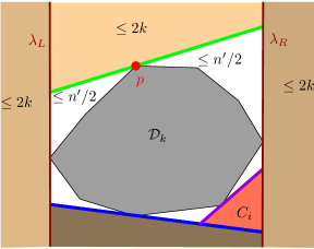
Figure 1: The polygon $\mathcal{D}_{k}$ and the decomposition of its complement.

Each step of the construction picks a pocket that contains more than $2k$ points of $P$, finds a line $\ell$ that supports $\mathcal{D}_{k}$ at a vertex of the pocket, and subdivides the pocket into two sub-pockets and a third piece that lies on the other side of $\ell$. The line $\ell$ is chosen so that the two resulting sub-pockets contain an equal number of points of $P$. The third piece, which clearly contains at most $2k$ points of $P$ (see Lemma 3.2), is taken to be the next polygon $\widehat{C}_{i+1}$, and the construction continues in this manner until each pocket has at most $2k$ points. We refer to the polygons $\widehat{C}_{i}$ constructed up to this point as non-terminal. We then terminate the construction, adding all the pockets to the output collection of polygons, referring to them as terminal polygons. Note that each non-terminal $\widehat{C}_{i}$ is a (possibly unbounded) triangle, having a “base” whose relative interior passes through a vertex of $\mathcal{D}_{k}$, and two other sides, each of which is a portion of a base of an earlier triangle. The terminal polygons are pseudo-triangles, each bounded by two straight edges and by a “base” which is a connected portion of the boundary of $\mathcal{D}_{k}$, possibly consisting of several edges. See Figure 1.

We claim that each line $\ell$ intersects at most $O(\log(n/k))$ polygons. For this, define the weight $w(\widehat{C}_{i})$ of a non-terminal polygon $\widehat{C}_{i}$, for $i\geq 3$, to be the number of points of $P$ in the pocket that was split when $\widehat{C}_{i}$ was created; the weight of each terminal polygon is the number of points of $P$ that it contains, which is at most $2k$. Define the level of $\widehat{C}_{i}$ to be $\left\lfloor{\log_{2}w(\widehat{C}_{i})}\right\rfloor$. It is easily checked that $\ell$ crosses at most two terminal polygons (two if it crosses $\mathcal{D}_{k}$ and at most one if it misses $\mathcal{D}_{k}$), and it can cross both (non-base) sides of at most one (terminal or non-terminal) polygon. Any other polygon $\widehat{C}_{i}$ crossed by $\ell$ is such that $\ell$ enters it through its base, reaching it from another polygon whose level is, by construction, strictly smaller than that of $\widehat{C}_{i}$. Since there are only $O(\log(n/k))$ distinct levels, the claim follows.

It is easy to verify that the convex hulls $C_{1}={\cal CH}(\widehat{C}_{1}),\ldots,C_{u}={\cal CH}(\widehat{C}_{u})$ are triangles with pairwise disjoint interiors, which have the required properties. ∎

Lemma 3.4

Let $1\leq k\leq n$ be a prespecified parameter. One can construct a spanning tree $\mathcal{T}$ for $P^{\prime}=P\setminus\mathcal{D}_{k}$, such that each line intersects at most $O(\sqrt{k}\log(n/k))$ edges of $\mathcal{T}$.

Proof.

Construct the decomposition of $P\setminus\mathcal{D}_{k}$ into $u$ covering triangles $C_{1},\ldots,C_{u}$, using Lemma 3.3.

For each $i=1,\ldots,u$, construct a spanning tree $\mathcal{T}_{i}$ of $P\cap C_{i}$ with crossing number $O(k^{1/2})$, using Theorem 3.1. In addition, connect one point of $P\cap C_{i}$ to an arbitrary vertex of ${\partial}{C_{i}}\cap{\partial}{\mathcal{D}_{k}}$. Since ${\cal CH}(P\cap C_{i})$ and ${\cal CH}(P\cap C_{j})$ are disjoint, for $i\neq j$, it follows that no pair of edges of any pair of (the plane embeddings of the) trees among $\mathcal{T}_{1},\ldots,\mathcal{T}_{u}$ cross each other.

Let $G$ be the planar straight-line graph formed by the union of ${\partial}{\mathcal{D}_{k}},\mathcal{T}_{1},\ldots,\mathcal{T}_{u}$, plus the connecting segments just introduced, and let $\mathcal{T}^{*}$ be a spanning tree of $G$; the vertex set of $\mathcal{T}^{*}$ contains $P\setminus\mathcal{D}_{k}$.

Let $\ell$ be a line in the plane. The proof of the preceding lemma implies that $\ell$ intersects at most $O(\log(n/k))$ of the polygons $C_{i}$. Hence, $\ell$ crosses at most two edges of ${\partial}{\mathcal{D}_{k}}$, at most $O(\log(n/k))$ of the connecting segments, and it can cross edges of at most $O(\log(n/k))$ trees $\mathcal{T}_{i}$, for $i=1,\ldots,u$. Since $\ell$ crosses at most $O(k^{1/2})$ edges of each such tree, we conclude that $\ell$ crosses at most $O(\sqrt{k}\log(n/k))$ edges of $\mathcal{T}^{*}$.

Finally, we get rid of the extra “Steiner vertices” of $\mathcal{T}^{*}$ (those not belonging to $P\setminus\mathcal{D}_{k}$) in a straightforward manner, by making $\mathcal{T}^{*}$ a rooted tree, at some point of $P\setminus\mathcal{D}_{k}$, and by replacing each path connecting a point $u\in P\setminus\mathcal{D}_{k}$ to an ancestor $v\in P\setminus\mathcal{D}_{k}$, where all inner vertices of the path are Steiner points, by the straight segment $uv$. This produces a straight-edge spanning tree $\mathcal{T}$ of $P\setminus\mathcal{D}_{k}$, whose crossing number is at most that of $\mathcal{T}^{*}$. ∎

Theorem 3.5

Given a set $P$ of $n$ points in the plane, one can construct a spanning tree $\mathcal{T}$ for $P$ such that any line $\ell$ crosses at most $O(\sqrt{w_{\ell}}\log(n/w_{\ell}))$ edges of $\mathcal{T}$. The tree $\mathcal{T}$ can be constructed in $O(n^{1+{\varepsilon}})$ (deterministic) time, for any fixed ${\varepsilon}>0$.

Proof.

We construct a sequence of subsets of $P$, as follows. Put $P_{0}=P$. At the $i$th step, $i\geq 1$, consider the polygon $Q_{i}=\mathcal{D}(P_{i-1},2^{i})$, and let $P_{i}=P_{i-1}\cap Q_{i}$. We stop when $P_{i}$ becomes empty. By construction, the $i$th step removes at least $2^{i}$ points from $P_{i-1}$, so $|P_{i}|\leq|P_{i-1}|-2^{i}$, and the process terminates in $O(\log n)$ steps.

For each $i$, construct a spanning tree $\mathcal{T}_{i}$ for $P_{i-1}\setminus Q_{i}$, using Lemma 3.4 (with $k=2^{i}$). Connect the resulting trees by straight segments into a single spanning tree $\mathcal{T}$ of $P$.

We claim that $\mathcal{T}$ is the desired spanning tree. Indeed, consider an arbitrary line $\ell$ of weight $k$. Observe that $\ell$ cannot cross any of the polygons $Q_{i}$, for $i>U=\left\lceil{\log_{2}k}\right\rceil$, since any line that crosses such a polygon must be of weight at least $2^{U+1}>k$, by Lemma 3.2(ii).

Thus $\ell$ crosses only the first $U$ layers of our construction. Hence, the number of edges of $\mathcal{T}$ that $\ell$ crosses is at most

$$\sum_{i=1}^{U}O\!\left({\sqrt{2^{i}}\log(n/2^{i})}\right)=O\!\left({\sum_{i=1}^{U}(\sqrt{2})^{i}(\log n-i)}\right)=O(\sqrt{k}\log(n/k)),$$

as is easily verified. This establishes the bound on the crossing number of $\ell$.

Running time.

Computing $Q_{i}$ can be done in the dual plane, by constructing the convex hulls of the levels $2^{i}$ and $n-2^{i}$ in the arrangement of the lines dual to the points of $P_{i-1}$. We use the algorithm of Matoušek [Mat91a], which constructs the convex hull of a level in $O\!\left({\left|{P_{i-1}}\right|\log^{4}n}\right)$ time, for a total of $O(n\log^{5}n)$ time. This also subsumes the time needed to construct $P_{i}$ from $P_{i-1}$, for all $i$. Next, we carry out the constructive proof of Lemma 3.3 for $P_{i-1}\setminus Q_{i}$, which can be implemented to run in $O(n\log^{O(1)}n)$ time. Finally, for each set in the cover, we apply the algorithm of [Wel92] to construct the corresponding subtree with low crossing number. This takes $O(m^{1+{\varepsilon}})$ time for a set of size $m$, for any fixed ${\varepsilon}>0$. We continue in this fashion, as described in the first part of the proof. It is now easy to verify that the resulting construction takes overall $O(n^{1+{\varepsilon}})$ time, for any fixed ${\varepsilon}>0$. ∎

3.1.1 The underlying partition and a counterexample in three dimensions

The main technical step in the construction of Theorem 3.5 is the partition of the set of $k$-shallow points of $P$, namely, those that are contained in some halfplane with at most $k$ points of $P$, into subsets, each containing at most $2k$ points, so that any line crosses the convex hulls of at most $O(\log(n/k))$ of these subsets.

It is natural to try to extend this construction to three (or higher) dimensions. However, as we show next, there are examples of point sets in ${\mathbb{R}}^{3}$ where no such partition exists, even when the points are in convex position.

To see this, let $m$ be an integer, and put $n=m^{2}$. Define

$$P=\left\{{(i,j,i^{2}+j^{2})\mid i,j=1,\ldots,m}\right\}.$$

That is, $P$ is the set of the vertices of the $m\times m$ integer grid in the $xy$-plane, lifted to the standard (convex) paraboloid $z=x^{2}+y^{2}$. Thus, all points of $P$ are in convex position (and are thus $1$-shallow).

Let $k>1$ be an arbitrary parameter, and consider any partition $\mathcal{P}=\left\{{Q_{1},\ldots,Q_{u}}\right\}$ of $P$ into $u=\Theta(n/k)$ sets, where $k\leq\left|{Q_{i}}\right|\leq 2k$, for $i=1,\ldots,u$. Let $C_{i}$ denote the two-dimensional convex hull of the projection of $Q_{i}$ onto the $xy$-plane, for $i=1,\ldots,u$. The sum of the $x$-span and the $y$-span of $C_{i}$ is at least $\sqrt{\left|{Q_{i}}\right|}$ (or else there would be no room for $Q_{i}$ to contain all its points). Hence, the total length of these spans of $C_{1},\ldots,C_{u}$ is at least $\Omega((n/k)\sqrt{k})=\Omega(n/\sqrt{k})$. Consider the $2m-2$ vertical planes $x=1+1/2,x=2+1/2,\ldots,x=m-1+1/2$, and $y=1+1/2,y=2+1/2,\ldots,y=m-1+1/2$. Clearly, the overall number of intersection points between the boundaries of the $C_{i}$’s and these planes is proportional to the sum of their $x$-spans and $y$-spans. Hence, there is a plane in this family that intersects $\Omega((n/\sqrt{k})/\sqrt{n})=\Omega(\sqrt{n/k})$ sets among $C_{1},\ldots,C_{u}$, and thus it intersects the $\Omega(\sqrt{n/k})$ corresponding convex hulls among ${\cal CH}(Q_{1}),\ldots,{\cal CH}(Q_{u})$.

Note that a similar argument can be applied to the set of the vertices of the $m^{1/3}\times m^{1/3}\times m^{1/3}$ integer lattice. In this case, for any partition of this set of the above kind, there always exists a plane that crosses the convex hulls of at least $\Omega((n/k)^{2/3})$ of the subsets. (This matches the upper bound in the partition theorem of Matoušek [Mat92].) Of course, here, (most of) the points are not shallow.

To summarize, there exist sets $P$ of $n$ points in convex position in 3-space (so they are all $1$-shallow), such that any partition of $P$ into sets of size (roughly) $k$ will have a plane that crosses at least $\Omega(\sqrt{n/k})$ sets in the partition. (Without the convex position, or shallowness, assumption, there exist sets for which this crossing number is at least $\Omega((n/k)^{2/3})$.) We do not know whether this lower bound is worst-case tight. That is, can a set $P$ of $n$ $k$-shallow points in 3-space be partitioned into $\Theta(n/k)$ subsets, so that no plane separates more than $O(\sqrt{n/k})$ subsets? If this were the case, applying the standard construction of spanning trees with small crossing numbers to each subset would result in a spanning tree with crossing number $O(n^{1/2}k^{1/6})$.

Note that this still leaves open the (more modest) possibility of a partition which is “depth sensitive”, that is, a partition into subsets of size roughly $k$, with the property that any halfspace that contains $m$ points crosses at most (or close to) $O((m/k)^{2/3})$ sets in the partition.

3.2 Relative $(p,{\varepsilon})$-approximations for halfplanes

We can turn the above construction of a spanning tree with small relative crossing number into a construction of a relative $(p,{\varepsilon})$-approximation for a set of points in the plane and for halfplane ranges, as follows.

Let $P$ be a set of $n$ points in the plane, and let $\mathcal{T}$ be a spanning tree of $P$ as provided in Theorem 3.5. We replace $\mathcal{T}$ by a perfect matching $M$ of $P$, with the same relative crossing number, i.e., the number of pairs of $M$ that are separated by a halfplane of weight $k$ is at most $O(\sqrt{k}\log(n/k))$. This is done in a standard manner—we first convert $\mathcal{T}$ to a spanning path whose relative crossing number is at most twice larger than the crossing number of $\mathcal{T}$, and then pick every other edge of the path.

We now construct a coloring of $P$ with low discrepancy, by randomly coloring the points in each pair of $M$. Specifically, each pair is randomly and independently colored either as $-1,+1$ or as $+1,-1$, with equal probability. The standard theory of discrepancy (see [Cha01]) yields the following variant.

Lemma 3.6

Given a set $P$ of $n$ points in the plane, one can construct a coloring $\chi:\;P\mapsto\{-1,1\}$, such that, for any halfplane $h$,

$$\chi(h\cap P)=O(|h\cap P|^{1/4}\log n).$$

The coloring is balanced—each color class consists of exactly $n/2$ points of $P$.

Proof.

As shown in [Mat99], if a halfplane $h$ crosses $t$ edges of the matching, then its discrepancy is $O(\sqrt{t\log n})$, with high probability. As shown above, $t=O(\sqrt{k}\log(n/k))$, for $k=|h\cap P|$, so the discrepancy of $h$ is, with high probability, $O\!\left({\sqrt{\sqrt{k}\log(n/k)\log n}}\right)=O(k^{1/4}\log n)$. ∎

We need the following fairly trivial technical lemma.

Lemma 3.7

For any $x\geq 0$, $y>0$, and $0<p<1$, we have $x^{p}<\!\left({x+y}\right)/{y^{1-p}}$.

Proof.

Observe that $\displaystyle x^{p}<(x+y)^{p}=\frac{x+y}{\!\left({x+y}\right)^{1-p}}\leq\frac{x+y}{y^{1-p}}$. ∎

As we next show, the improved discrepancy bound of Lemma 3.6 leads to an improved bound on the size of $(\nu,\alpha)$-samples for our range space, and, consequently, for the size of relative $(p,{\varepsilon})$-approximations.

Theorem 3.8

Given a set $P$ of $n$ points in the plane, and parameters $0<\alpha<1$ and $0<\nu<1$, one can construct a $(\nu,\alpha)$-sample $Z\subseteq P$ of size $O\!\left({\frac{1}{\alpha^{4/3}\nu}\log^{4/3}\frac{1}{\alpha\nu}}\right)$.

Proof.

Following one of the classical constructions of ${\varepsilon}$-approximations (see [Cha01], we repeatedly halve $P$, until we obtain a subset of size as asserted in the theorem, and then argue that the resulting set is a $(\nu,\alpha)$-sample. Formally, set $P_{0}=P$, and partition $P_{i-1}$ into two equal halves, using Lemma 3.6; let $P_{i}$ and $P_{i}^{\prime}$ denote the two halves (consisting of the points that are colored $+1$, $-1$, respectively). We keep $P_{i}$, remove $P^{\prime}_{i}$, and continue with the halving process. Let $n_{i}=\left|{P}\right|/2^{i}$ denote the size of $P_{i}$. For any halfplane $h$, we have

$$\biggl{|}\left|{P_{i}\cap h}\right|-\left|{P_{i}^{\prime}\cap h}\right|\biggr{|}\leq c\ \left|{h\cap P_{i}}\right|^{1/4}\log n_{i},$$

where $c$ is some appropriate constant. Recalling that

$$\overline{P_{i}}\!\left({h}\right)=\frac{\left|{h\cap P_{i}}\right|}{\left|{P_{i}}\right|}\quad\mbox{and}\quad\overline{P_{i}^{\prime}}\!\left({h}\right)=\frac{\left|{h\cap P_{i}^{\prime}}\right|}{\left|{P_{i}^{\prime}}\right|},$$

and that $\left|{P_{i}}\right|=\left|{P_{i}^{\prime}}\right|$, this can be rewritten as

$$\left|{\overline{P_{i}}\!\left({h}\right)-\overline{P_{i}^{\prime}}\!\left({h}\right)}\right|\leq c\frac{\overline{P_{i}}\!\left({h}\right)^{1/4}}{n_{i}^{3/4}}\log n_{i}.$$

Since $P_{i-1}=P_{i}\cup P_{i}^{\prime}$, we have

$$\overline{P_{i-1}}\!\left({h}\right)=\frac{\left|{h\cap P_{i-1}}\right|}{\left|{P_{i-1}}\right|}=\frac{\left|{h\cap P_{i}}\right|}{2\left|{P_{i}}\right|}+\frac{\left|{h\cap P_{i}^{\prime}}\right|}{2\left|{P_{i}^{\prime}}\right|}=\frac{1}{2}\!\left({\overline{P_{i}}\!\left({h}\right)+\overline{P_{i}^{\prime}}\!\left({h}\right)}\right).$$

Since $\nu>0$, we have

$$\left|{\overline{P_{i-1}}\!\left({h}\right)-\overline{P_{i}}\!\left({h}\right)}\right| =\frac{\left|{\overline{P_{i}}\!\left({h}\right)-\overline{P_{i}^{\prime}}\!\left({h}\right)}\right|}{2}=\frac{c\overline{P_{i}}\!\left({h}\right)^{1/4}}{2n_{i}^{3/4}}\log n_{i}.$$

Applying Lemma 3.7, with $p=1/4$, $x=\overline{P_{i}}\!\left({h}\right)$, and $y=\nu$, the last expression is at most

$$\frac{c\log n_{i}}{2n_{i}^{3/4}}\cdot\frac{\overline{P_{i}}\!\left({h}\right)+\nu}{\nu^{3/4}}\leq\frac{c\log n_{i}}{2\!\left({\nu n_{i}}\right)^{3/4}}\!\left({\overline{P_{i-1}}\!\left({h}\right)+\overline{P_{i}}\!\left({h}\right)+\nu}\right).$$

This implies that $\displaystyle d_{\nu}(\overline{P_{i-1}}\!\left({h}\right),\overline{P_{i}}\!\left({h}\right))\leq\frac{c\log n_{i}}{2\!\left({\nu n_{i}}\right)^{3/4}}$. The triangle inequality then implies that

$$d_{\nu}(\overline{P}\!\left({h}\right),\overline{P_{i}}\!\left({h}\right))\leq\sum_{k=1}^{i}d_{\nu}(\overline{P_{k-1}}\!\left({h}\right),\overline{P_{k}}\!\left({h}\right))\leq\frac{c}{2\nu^{3/4}}\sum_{k=1}^{i}\frac{\log n_{k}}{n_{k}^{3/4}}=O\!\left({\frac{\log n_{i}}{\!\left({\nu n_{i}}\right)^{3/4}}}\right)\leq\alpha,$$

for $n_{i}=\Omega\!\left({\frac{1}{\nu\alpha^{4/3}}\log^{4/3}\frac{1}{\alpha\nu}}\right)$. The theorem then follows by taking $Z$ to be the smallest $P_{i}$ which still satisfies this size constraint. ∎

Using Theorem 2.9, we thus obtain:

Corollary 3.9

Given a set $P$ of $n$ points in the plane, and parameters $0<{\varepsilon}<1$ and $0<p<1$, one can construct a relative $(p,{\varepsilon})$-approximation $Z\subseteq P$ of size $O\!\left({\frac{1}{{\varepsilon}^{4/3}p}\log^{4/3}\frac{1}{{\varepsilon}p}}\right)$.

Remark: One can speed up the construction of the relative $(p,{\varepsilon})$-approximation of Corollary 3.9, by first drawing a random sample of slightly larger size, which is guaranteed, with high probability, to be a relative approximation of the desired kind, and then use halving to decimate it to the desired size. Implemented carefully, this takes $O\!\left({n+\!\left({\frac{1}{{\varepsilon}^{2}p}\log n}\right)^{3}}\right)$ time, and thus produces a relative $(p,{\varepsilon})$-approximation, with high probability, of the desired size $O\!\left({\frac{1}{{\varepsilon}^{4/3}p}\log^{4/3}\frac{1}{{\varepsilon}p}}\right)$.

In fact, the preceding analysis leads to an improved bound for sensitive approximations for our range space. The improvement is in terms of the quality of the “sensitivity” of the approximation, which is achieved at the cost of a slight increase (by a sublogarithmic factor) in its size, as compared to the standard bound, provided in Theorem 2.13. That is, we have:

Theorem 3.10

Let $P$ be a set of $n$ points in the plane, and let ${\varepsilon}>0$ be a parameter. One can compute a subset $Z\subseteq P$ of size $O\!\left({(1/{\varepsilon}^{2})\log^{4/3}(1/{\varepsilon})}\right)$, such that for any halfplane $h$, we have $\displaystyle\left|{\overline{P}\!\left({h}\right)-\overline{Z}\!\left({h}\right)}\right|\leq\frac{1}{2}\left({\varepsilon}^{3/2}\overline{P}\!\left({h}\right)^{1/4}+{\varepsilon}^{2}\right)$.

Proof.

Fix parameters $0<\alpha<1$ and $\nu>0$, and Apply the construction of Theorem 3.8 until we get a subset $Z$ of size $m=O\!\left({(1/{\varepsilon}^{2})\log^{4/3}(1/{\varepsilon})}\right)$; the constant of proportionality will be determined by the forthcoming considerations.

The key observation is that $Z$ is a $(\nu,\alpha)$-sample for any $0<\alpha<1$ and $\nu>0$ that satisfy $m=\Omega\!\left({\frac{1}{\alpha^{4/3}\nu}\log^{4/3}\frac{1}{\alpha\nu}}\right)$, because the construction is oblivious to the individual values of $\alpha$ and $\nu$, and just requires that the size of the sample remains larger than the above threshold.

Using this observation, we proceed to show that $Z$ satisfies the property asserted in the theorem. So let $h$ be a halfplane. Suppose first that $\overline{P}\!\left({h}\right)\leq{\varepsilon}^{2}/2$. By Corollary 3.9, $Z$ is a relative $({\varepsilon}^{2},1/2)$-approximation to $P$, with an appropriate choice of the constant of proportionality (note the change of roles of “$p$” and “${\varepsilon}$”). This implies that $\left|{\overline{Z}\!\left({h}\right)-\overline{P}\!\left({h}\right)}\right|\leq{\varepsilon}^{2}/2$.

Suppose then that $p_{h}=\overline{P}\!\left({h}\right)>{\varepsilon}^{2}/2$, and set ${\varepsilon}_{h}={\varepsilon}^{3/2}/p_{h}^{3/4}$. Observe that

$$\frac{1}{{{\varepsilon}_{h}}^{4/3}p_{h}}\log^{4/3}\frac{1}{{\varepsilon}_{h}p_{h}}=O\left(\frac{1}{{\varepsilon}^{2}}\log^{4/3}\frac{1}{{\varepsilon}}\right)=O(m).$$

Thus, with an appropriate choice of the constant of proportionality for $m$, $Z$ is a relative $(p_{h},{\varepsilon}_{h}/2)$-approximation, which implies that

$$\left|{\overline{P}\!\left({h}\right)-\overline{Z}\!\left({h}\right)}\right|\leq\frac{1}{2}{\varepsilon}_{h}\overline{P}\!\left({h}\right)=\frac{{\varepsilon}^{3/2}}{2p_{h}^{3/4}}\overline{P}\!\left({h}\right)=\frac{1}{2}{\varepsilon}^{3/2}\overline{P}\!\left({h}\right)^{1/4},$$

as asserted. ∎

This compares favorably with the result of Brönnimann et al. [Brö95, BCM99], which in this case implies that there exists a subset of size $O((1/{\varepsilon}^{2})\log(1/{\varepsilon}))$ such that, for each halfplane $h$, we have ${\displaystyle\left|{\overline{P}\!\left({h}\right)-\overline{Z}\!\left({h}\right)}\right|\leq({\varepsilon}/2)\!\left({\overline{P}\!\left({h}\right)^{1/2}+{\varepsilon}}\right)}$. Our bound is smaller when $\overline{P}\!\left({h}\right)>{\varepsilon}^{2}$ and is the same otherwise.

4 Relative $(p,{\varepsilon})$-approximations in higher dimensions

4.1 Relative $(p,{\varepsilon})$-approximations in ${\mathbb{R}}^{3}$

The construction in higher dimensions is different from the planar one, because of our present inability to extend the construction of spanning trees with low relative crossing number to three or higher dimension. For this reason we use the following different strategy.

We say that a hyperplane $h$ separates a set $Q\subseteq{\mathbb{R}}^{d}$ if $h$ intersects the interior of ${\cal CH}(Q)$; that is, each of the open halfspaces that $h$ bounds intersects $Q$.

The main technical step in the construction is given in the following theorem.

Theorem 4.1

Let $P$ be a set of $n$ points in ${\mathbb{R}}^{3}$, and let $0<{\varepsilon}<1$, $0<p<1$ be given parameters. Then there exists a set $Z\subseteq P$, of size $\displaystyle O\!\left({\frac{1}{{\varepsilon}^{3/2}p}\log^{3/2}\frac{1}{{\varepsilon}p}}\right)$, such that, for any halfspace $h$ with $\overline{P}\!\left({h}\right)\leq p$, we have

$$\left|{\overline{Z}\!\left({h}\right)-\overline{P}\!\left({h}\right)}\right|\leq{\varepsilon}p.$$ (4)

Remark: Let us note right away the difference between Eq. (4) and the situation in the preceding sections. That is, up to now we have handled ranges of measure at least $p$, whereas Eq. (4) applies to ranges of measure at most $p$. This issue requires a somewhat less standard construction, that will culminate in a sequence of approximation sets, each catering to a different range of halfspace measures. Nevertheless, the overall size of these sets will satisfy the above bound, and the cost of accessing them will be small.

Proof.

Put $k=\lfloor np\rfloor$, and apply the shallow partition theorem of Matoušek [Mat91b], to obtain a partition of $P$ into $s\leq n/k=O(1/p)$ subsets $P_{1},\ldots,P_{s}$, each of size between $k+1$ and $2k$, such that any $k$-shallow halfspace $h$ (namely, a halfspace that contains at most $k$ points of $P$) separates at most $c\log s$ subsets, for some absolute constant $c$. (Note that if $h$ meets any $P_{i}$, it has to separate it, because $h$ is too shallow to fully contain $P_{i}$.) Without loss of generality, we can carry out the construction so that the size of each $P_{i}$ is even.

We then construct, for each subset $P_{i}$, a spanning tree of $P_{i}$ with crossing number $O(k^{2/3})$ [CW89, Wel92], and convert it, as in the preceding section, to a perfect matching of $P_{i}$, with the same asymptotic bound on its crossing number, which is the maximum number of pairs in the matching that a halfspace separates. We combine all these perfect matchings to a perfect matching of the entire set $P$.

We then color each matched pair independently, as above, coloring at random one of its points by either $-1$ or $+1$, with equal probabilities, and the other point by the opposite color. Let $R_{1}$ be the set of points colored $-1$; we have $\left|{R_{1}}\right|=n/2$. With high probability, the discrepancy of any halfspace $h$ is at most $\sqrt{6\xi(h)\ln(2n)}$, where $\xi(h)$ is the crossing number of $h$ (see [Cha01]); we may assume that the coloring does indeed have this property. (If we do not care about the running time, we can verify that the constructed set has the required property, and if not regenerate it.)

Hence, if $h$ is a $k$-shallow halfspace, then, by construction, $\xi(h)=O\!\left({k^{2/3}\log s}\right)$, because $h$ separates $O(\log s)$ subsets and crosses $O(k^{2/3})$ edges of the spanning tree of each of them. Hence the discrepancy of any $k$-shallow halfspace $h$ is $O(k^{1/3}\log n)$.

We continue recursively in this manner for $j$ steps, producing a sequence of subsets $R_{0}=P,R_{1},\ldots,R_{j}$, where $R_{i}$ is obtained from $R_{i-1}$ by applying the partitioning of [Mat91b] with a different parameter $k_{i-1}$, and then by using the above coloring procedure on the resulting perfect matching. We take $k_{i-1}=k\min\{\mathsf{c}/2^{i-1},1\}$, where $\mathsf{c}$ is the constant derived in the following lemma. (The bound asserted in the lemma holds with high probability if we do not verify that our colorings have small discrepancy, and is worst-case if we do verify it.)

Lemma 4.2

There exists an absolute constant $\mathsf{c}$ such that any $pn$-shallow halfspace satisfies, for any $i\leq j$,

$$\left|{h\cap R_{i}}\right|\leq\frac{\mathsf{c}pn}{2^{i}},$$

where $j$ is the largest index satisfying $n_{j}\geq\frac{2}{p}\ln^{3/2}\frac{1}{p}$, where $n_{j}=\left|{P_{j}}\right|=n/2^{j}$.

Proof.

Delegated to Appendix A.1. ∎

The lemma implies that $h$ is $k_{i}$-shallow in each of the subsets $R_{1},\ldots,R_{j}$, so we can use the above bound on the discrepancy of $h$ with respect to each of these subsets. (The reader can note the similarity between the forthcoming analysis and the proof of Lemma 4.2.) We thus have

$$\left|{\overline{P}\!\left({h}\right)-\overline{R_{1}}\!\left({h}\right)}\right| = \frac{\biggl{|}\left|{h\cap P}\right|-2\left|{h\cap R_{1}}\right|\biggr{|}}{\left|{P}\right|}=\frac{{\rm\chi}(h,P)}{n}=O\!\left({\frac{k^{1/3}\log n}{n}}\right)$$

$$\left|{\overline{R_{1}}\!\left({h}\right)-\overline{R_{2}}\!\left({h}\right)}\right| = \frac{{\rm\chi}(h,R_{1})}{\left|{R_{1}}\right|}=O\!\left({\frac{k_{1}^{1/3}\log(n/2)}{n/2}}\right)$$

$$\vdots$$

$$\left|{\overline{R_{j-1}}\!\left({h}\right)-\overline{R_{j}}\!\left({h}\right)}\right| = \frac{{\rm\chi}(h,R_{j-1})}{\left|{R_{j-1}}\right|}=O\!\left({\frac{2^{j-1}k_{j-1}^{1/3}\log(n/2^{j-1})}{n}}\right).$$

Substituting $k_{i}=k\min\{\mathsf{c}/2^{i},1\}$, for each $i$, and adding up the inequalities, it is easily checked that the last right-hand side dominates the sum (compare with the analysis in the proof of Theorem 3.5), so we obtain, using the triangle inequality,

$$\left|{\overline{P}\!\left({h}\right)-\overline{R_{j}}\!\left({h}\right)}\right|=O\!\left({\frac{2^{2j/3}k^{1/3}\log(n/2^{j-1})}{n}}\right).$$

We choose $j$ to be the largest index for which this bound is at most ${\varepsilon}p\leq{\varepsilon}k/n$. That is, $2^{j}=O\!\left({\frac{{\varepsilon}^{3/2}pn}{\log^{3/2}(n/2^{j})}}\right)$. Note that this can be rewritten as $\frac{n_{j}}{\log^{3/2}n_{j}}=\Omega\left(\frac{1}{{\varepsilon}^{3/2}p}\right)$, which implies that $n_{j}\geq\frac{2}{p}\ln^{3/2}\frac{1}{p}$, as required in Lemma 4.2, provided that ${\varepsilon}$ is smaller than some appropriate absolute constant. Hence, since $j$ was chosen as large as possible, the size of $R_{j}$ is

$$\left|{R_{j}}\right|=\frac{n}{2^{j}}=O\!\left({\frac{\log^{3/2}(n/2^{j})}{{\varepsilon}^{3/2}p}}\right)=O\!\left({\frac{1}{{\varepsilon}^{3/2}p}\log^{3/2}\frac{1}{{\varepsilon}p}}\right).$$

Taking $Z=R_{j}$ completes the proof of Theorem 4.1. ∎

4.1.1 How to obtain a relative approximate count.

Construction.

The preceding construction used a fixed $k=pn$, and assumed that the query halfspace is at most $k$-shallow. However, our goal is to construct a subset that caters to all halfspaces whose measure is at least some given threshold. While unable to meet this goal exactly, with a single subset, we almost get there, in the following manner. Let $p$ be the given threshold parameter. We consider the geometric sequence $\{p_{t}\}_{t\geq 0}$, where $p_{t}=2^{t}p$; the last (largest) element is $\approx 1/2$, and its index is $t_{\rm max}=O\!\left({\log\frac{1}{p}}\right)$. For each $t$, we construct a relative $(p_{t},c{\varepsilon})$-approximation $Z_{t}$ for $P$, as in Theorem 4.1, where $c$ is a sufficiently small constant, whose value will be determined later. Clearly, the overall size of all these sets is dominated by the size of the first set, namely, it is

$$O\!\left({\frac{1}{{\varepsilon}^{3/2}p}\log^{3/2}\frac{1}{{\varepsilon}p}}\right).$$

We output the entire sequence $Z_{0},Z_{1},\ldots$, as a substitute for a single relative $(p,{\varepsilon})$-approximation, and use it as follows.

Answering a query.

Let $h$ be a given halfspace, so that $w=\left|{h\cap P}\right|\geq pn$. Let $t\geq 1$ be the index (initially unknown) for which $p_{t-1}n\leq w<p_{t}n$. Thus $h$ is $p_{t}n$-shallow, and is also $p_{s}n$-shallow, for every $s\geq t$. Hence, if we use the set $Z_{s}$, for each $s\geq t$, to approximate $w$, we get, by Theorem 4.1, a count $C_{s}:=\overline{Z_{s}}\!\left({h}\right)\cdot\left|{P}\right|$, which satisfies $\left|{C_{s}-w}\right|\leq c{\varepsilon}p_{s}n$. In other words, we have

$$C_{s}-c{\varepsilon}p_{s}n\leq w\leq C_{s}+c{\varepsilon}p_{s}n,$$

for each $s\geq t$.

To answer the query, we access the sets $Z_{t_{\rm max}},Z_{{t_{\rm max}}-1},\ldots$, in decreasing order, and find the largest index $s$ satisfying

$$c{\varepsilon}p_{s}n<\frac{4}{5}C_{s}.$$ (5)

We return $C_{s}$ as the desired approximate count.

Analysis.

We claim that Eq. (5) must hold at $s=t$, assuming ${\varepsilon}<\frac{1}{8c}$. Indeed, since $\frac{1}{2}p_{t}n\leq w<p_{t}n$, we have

$$C_{t}+c{\varepsilon}p_{t}n\geq w\geq\frac{1}{2}p_{t}n,\quad\text{or}\quad C_{t}\geq\!\left({\frac{1}{2}-c{\varepsilon}}\right)p_{t}n.$$

Hence, $C_{t}-c{\varepsilon}p_{t}n\geq\!\left({\frac{1}{2}-2c{\varepsilon}}\right)p_{t}n$. On the other hand, $C_{t}\leq c{\varepsilon}p_{t}n+w<(1+c{\varepsilon})p_{t}n$. Combining these two inequalities, we obtain

$$C_{t}-c{\varepsilon}p_{t}n>\frac{\frac{1}{2}-2c{\varepsilon}}{1+c{\varepsilon}}C_{t}>\frac{1}{5}C_{t},$$

if ${\varepsilon}<\frac{1}{8c}$, as assumed. Our choice of $s$ thus satisfies $s\geq t$. Moreover, we have

$$\frac{1}{5}C_{s}<C_{s}-c{\varepsilon}p_{s}n\leq w\leq C_{s}+c{\varepsilon}p_{s}n<\frac{9}{5}C_{s}.$$

This determines $w$, up to a factor of $9$, which thus determines the correct index $t$ (up to $\pm O(1)$). In fact, as our query answering procedure actually does, we do not have to find the exact value of $t$, because we use a smaller value of ${\varepsilon}$ in the construction of the sets $Z_{s}$. Specifically, with an appropriate choice of $c$, we have $p_{t}>2cp_{s}$, so

$$C_{s}\leq w+c{\varepsilon}p_{s}n<w+\frac{1}{2}{\varepsilon}p_{t}n=w+{\varepsilon}p_{t-1}n\leq(1+{\varepsilon})w,$$

and, similarly,

$$C_{s}\geq w-c{\varepsilon}p_{s}n>w-\frac{1}{2}{\varepsilon}p_{t}n=w-{\varepsilon}p_{t-1}n\geq(1-{\varepsilon})w,$$

so $C_{s}$ is an ${\varepsilon}$-approximate count of $P\cap h$, establishing the correctness of our procedure. (The specific choice of $c$, which we do not spell out, can easily be worked out from the preceding analysis.)

Note that our structure also handles halfspaces $h$ with $w=|h\cap P|\leq pn$. Specifically, if we find an index $s$ satisfying Eq. (5) then $C_{s}$ is an ${\varepsilon}$-approximate count of $P\cap h$, as the preceding analysis shows. If no such $s$ is found then we must have $w\leq p_{1}n=pn$ (otherwise, as just argued, there would exist such an $s$ and the procedure would find it). In this case we have $|w-C_{1}|\leq{\varepsilon}pn$, and we return $C_{1}$ with the guarantee that (a) $w\leq pn$, and (b) $|w-C_{1}|\leq{\varepsilon}pn$.

Note that this constitutes a somewhat unorthodox approach—we have logarithmically many sets instead of a single one (although their combined size is asymptotically the same as that of the largest one), and we access them sequentially to find the one that gives the best approximation. An interesting useful feature of the construction is that, if the given halfspace $h$ has weight $w$ that satisfies $p_{t-1}n<w\leq p_{t}n$, then the approximate counting mechanism accesses sets whose overall size is only $O\!\left({\frac{1}{{\varepsilon}^{3/2}p_{t}}\log^{3/2}\frac{1}{{\varepsilon}p_{t}}}\right)$. That is, the larger $w$ is, the faster is the procedure.

To summarize, we have shown:

Theorem 4.3

Given a set $P$ of $n$ points in ${\mathbb{R}}^{3}$, and two parameters $0<{\varepsilon}<1$, $0<p<1$, we can construct $k=O\!\left({\log\frac{1}{p}}\right)$ subsets of $P$, $Z_{0},Z_{1},\ldots,Z_{k}$, of total size $O\!\left({\frac{1}{{\varepsilon}^{3/2}p}\log^{3/2}\frac{1}{{\varepsilon}p}}\right)$, so that, given any halfspace $h$ containing $qn$ points of $P$, we can find a set $Z_{t}$ that satisfies

$$\left|{\overline{Z_{t}}\!\left({h}\right)-\overline{P}\!\left({h}\right)}\right|\leq\begin{cases}{\varepsilon}\overline{P}\!\left({h}\right),&\mbox{if $q\geq p$}\\ {\varepsilon}p,&\mbox{if $q\leq p$}.\end{cases}$$

The (brute-force) time it takes to search for $Z_{t}$ and obtain the count $\left|{h\cap Z_{t}}\right|$ is

$$\begin{cases}O\!\left({\frac{1}{{\varepsilon}^{3/2}q}\log^{3/2}\frac{1}{{\varepsilon}q}}\right),&\mbox{if $q\geq p$}\\ O\!\left({\frac{1}{{\varepsilon}^{3/2}p}\log^{3/2}\frac{1}{{\varepsilon}p}}\right),&\mbox{if $q\leq p$}.\end{cases}$$

4.2 Higher dimensions

The preceding construction can be generalized to higher dimensions, with some complications. We first introduce the following parameters:

$$\gamma = 1+\frac{1-\frac{1}{d^{*}}}{1+\frac{1}{d}},\quad\text{where}\quad d^{*}=\lfloor d/2\rfloor,\text{~{} and ~{}}{\mu}=\frac{2d}{d+1}.$$

Note that, for $d\geq 4$, $1<\gamma<2$ (and tends to $2$ as $d$ increases), and ${\mu}<2$ (and tends to $2$ as $d$ increases).

The analogous version of Theorem 4.1 is:

Theorem 4.4

Let $P$ be a set of $n$ points in ${\mathbb{R}}^{d}$, $d\geq 4$, and let $0<{\varepsilon}<1$, $0<p<1$ be given parameters. Then there exists a set $Z\subseteq P$, of size $\displaystyle O\!\left({\frac{d^{{\mu}/2}}{{\varepsilon}^{\mu}p^{\gamma}}\log\frac{d}{{\varepsilon}p}}\right)$, such that, for any $pn$-shallow halfspace $h$, we have

$$\left|{\overline{Z}\!\left({h}\right)-\overline{P}\!\left({h}\right)}\right|\leq{\varepsilon}p,$$

provided that $n=\Omega\!\left({\frac{d^{{\mu}/2}}{p^{\gamma}}\log^{{\mu}/2}\frac{d}{p}}\right)$.

Proof.

As above, put $k=\lfloor np\rfloor$, and apply Matoušek’s shallow partition theorem [Mat91b], to obtain a partition of $P$ into $s=O(1/p)$ subsets $P_{1},\ldots,P_{s}$, each of size between $k+1$ and $2k$, such that any $k$-shallow halfspace separates at most $c(n/k)^{\beta}$ subsets, for some absolute constant $c$, where $\beta=1-1/\lfloor d/2\rfloor=1-1/d^{*}$. (As above, if $h$ meets any $P_{i}$, it has to separate it.) Also, we may assume that the size of each $P_{i}$ is even.

We then construct, for each subset $P_{i}$, a spanning path of $P_{i}$ with crossing number $O(k^{\alpha})$ [Wel92], for $\alpha=1-1/d$, convert it to a perfect matching of $P_{i}$, with the same asymptotic crossing number, and combine all these matchings to a perfect matching of $P$.

We then apply the same coloring scheme as in the three-dimensional case, and let $R_{1}$ be the set of points colored by $-1$; we have $\left|{R_{1}}\right|=n/2$. With high probability, the discrepancy of any halfspace $h$ is at most $\sqrt{2d\xi(h)\ln 2n}$, where $\xi(h)$ is the number of pairs in the matching that $h$ separates [Cha01]. If $h$ is $k$-shallow then, by construction, $\xi(h)=O\!\left({\sum_{i}k^{\alpha}(n/k)^{\beta}}\right)$. Hence the discrepancy of $h$ is

$$\chi(h,P)=O(\sqrt{d}k^{x}n^{y}\log^{1/2}n),\text{ ~{} for ~{}}x=\frac{1}{2}\!\left({\alpha-\beta}\right),\text{ and }y=\frac{1}{2}\beta.$$

We continue recursively in this manner for $j$ steps, producing, as above, a sequence of subsets $R_{0}=P,R_{1},\ldots,R_{j}$, where $R_{i}$ is obtained from $R_{i-1}$ by applying the partitioning of [Mat91b] with a different parameter $k_{i-1}$, and then by using the above coloring procedure on the resulting perfect matching. We take $k_{i-1}=k\min\{\mathsf{c}/2^{i-1},1\}$, where $\mathsf{c}$ is the constant derived in the following lemma. (As in the 3-dimensional case, if we want the proof of the theorem to be constructive, we either verify that each half-sample has the desired low discrepancy, and then the bounds are worst-case, or else the bounds hold with high probability.)

Lemma 4.5

There exists an absolute constant $\mathsf{c}$ such that any $pn$-shallow halfspace satisfies, for any $i\leq j$,

$$\left|{h\cap R_{i}}\right|\leq\frac{\mathsf{c}pn}{2^{i}},$$

where $j$ is the largest index satisfying $n_{j}=\Omega\!\left({\frac{d^{{\mu}/2}}{p^{\gamma}}\log^{{\mu}/2}\frac{d}{p}}\right)$, where $n_{j}=\left|{P_{j}}\right|=n/2^{j}$.

Proof.

Delegated to Appendix A.2. ∎

As in the 3-dimensional case, the lemma justifies the following chain of inequalities (note again the similarity between the proof of the lemma and the analysis below).

$$\left|{\overline{P}\!\left({h}\right)-\overline{R_{1}}\!\left({h}\right)}\right| = \frac{\biggl{|}\left|{h\cap P}\right|-2\left|{h\cap R_{1}}\right|\biggr{|}}{\left|{P}\right|}=\frac{{\rm\chi}(h,P)}{n}=O\!\left({\frac{\sqrt{d}k^{x}n^{y}\log^{1/2}n}{n}}\right)$$

$$\left|{\overline{R_{1}}\!\left({h}\right)-\overline{R_{2}}\!\left({h}\right)}\right| = \frac{{\rm\chi}(h,R_{1})}{\left|{R_{1}}\right|}=O\!\left({\frac{\sqrt{d}k_{1}^{x}(n/2)^{y}\log^{1/2}(n/2)}{n/2}}\right)$$

$$\vdots$$

$$\left|{\overline{R_{j-1}}\!\left({h}\right)-\overline{R_{j}}\!\left({h}\right)}\right| = \frac{{\rm\chi}(h,R_{j-1})}{\left|{R_{j-1}}\right|}=O\!\left({\frac{2^{j-1}\sqrt{d}k_{j-1}^{x}(n/2^{j-1})^{y}\log^{1/2}(n/2^{j-1})}{n}}\right).$$

Substituting $k_{i}=k\min\{\mathsf{c}/2^{i},1\}$, for each $i$, and adding up the inequalities, the last right-hand side dominates, so we obtain

$$\left|{\overline{P}\!\left({h}\right)-\overline{R_{j}}\!\left({h}\right)}\right|=O\!\left({\frac{2^{(1-x-y)j}\sqrt{d}k^{x}n^{y}\log^{1/2}(n/2^{j-1})}{n}}\right).$$

Substituting $k=pn$ and the values of $x$ and $y$, this is equal to

$$O\!\left({\frac{p^{x}\sqrt{d}\log^{1/2}n_{j}}{n_{j}^{1-\alpha/2}}}\right).$$

We choose the first $j$ so that this bound is at most ${\varepsilon}p$. That is,

$$\frac{n_{j}^{1-\alpha/2}}{\log^{1/2}n_{j}}=\Omega\!\left({\frac{\sqrt{d}}{{\varepsilon}p^{1-x}}}\right),$$

$$\text{or}\quad\left|{R_{j}}\right|=n_{j}=\Theta\!\left({\frac{d^{{\mu}/2}}{{\varepsilon}^{\mu}p^{\gamma}}\log^{{\mu}/2}\frac{d}{{\varepsilon}p}}\right).$$

We note that the choice of $n_{j}$ satisfies the lower bound constraint in Lemma 4.5. Hence, taking $Z=R_{j}$ completes the proof. ∎

Obtaining a relative approximate count is done exactly as in the three-dimensional case, producing a sequence of approximations, and searching through the sequence for the approximation which caters for the correct range of the size of $P\cap h$. We thus have the following result.

Theorem 4.6

Given a set $P$ of $n$ points in ${\mathbb{R}}^{d}$, and two parameters $0<{\varepsilon}<1$, $0<p<1$, we can construct $k=O\!\left({\log\frac{1}{p}}\right)$ subsets of $P$, $Z_{0},Z_{1},\ldots,Z_{k}$, of total size $O\!\left({\frac{d^{{\mu}/2}}{{\varepsilon}^{\gamma}p^{\mu}}\log^{{\mu}/2}\frac{1}{{\varepsilon}p}}\right)$, so that, given any halfspace $h$ containing $qn$ points of $P$, we can find a set $Z_{t}$ that satisfies

$$\left|{\overline{P}\!\left({h}\right)-\overline{Z_{t}}\!\left({h}\right)}\right|\leq\begin{cases}{\varepsilon}\overline{P}\!\left({h}\right),&\mbox{if $q\geq p$}\\ {\varepsilon}p,&\mbox{if $q\leq p$}.\end{cases}$$

The (brute-force) time it takes to search for $Z_{t}$ and obtain the count $\left|{h\cap Z_{t}}\right|$ is

$$\begin{cases}O\!\left({\frac{d^{{\mu}/2}}{{\varepsilon}^{\gamma}q^{\mu}}\log^{{\mu}/2}\frac{1}{{\varepsilon}q}}\right),&\mbox{if $q\geq p$}\\ O\!\left({\frac{d^{{\mu}/2}}{{\varepsilon}^{\gamma}p^{\mu}}\log^{{\mu}/2}\frac{1}{{\varepsilon}p}}\right),&\mbox{if $q\leq p$}.\end{cases}$$

Discussion.

We have two competing constructions, the “traditional” one, with $N=\Theta\!\left({\frac{d}{{\varepsilon}^{2}p}\log\frac{1}{p}}\right)$ elements (see Section 2), and the new one, with $N^{\prime}=\Theta\!\left({\frac{d^{{\mu}/2}}{{\varepsilon}^{\mu}p^{\gamma}}\log^{{\mu}/2}\frac{d}{{\varepsilon}p}}\right)$ elements. The new construction is better, in terms of the size of the approximation, when

$$\frac{d^{{\mu}/2}}{{\varepsilon}^{\mu}p^{\gamma}}\log^{{\mu}/2}\frac{d}{{\varepsilon}p}<\frac{d}{{\varepsilon}^{2}p}\log\frac{1}{p}$$

(for simplicity, we ignore the constants of proportionality). For further simplicity, assume that $p$ is not much larger than ${\varepsilon}$, so that $\log\frac{d}{{\varepsilon}p}$ and $\log\frac{1}{p}$ are roughly the same, up to some constant factor. Then we replace the above condition by

$$\frac{d^{{\mu}/2}}{{\varepsilon}^{\mu}p^{\gamma}}\log^{{\mu}/2}\frac{d}{{\varepsilon}p}<\frac{d}{{\varepsilon}^{2}p}\log\frac{d}{{\varepsilon}p}.$$

Substituting the values of $\gamma$ and ${\mu}$, and simplifying the expressions, this is equivalent to

$$\frac{1}{p^{d(1-1/d^{*})}}<\frac{d}{{\varepsilon}^{2}}\log\frac{d}{{\varepsilon}p},\quad\text{or}\quad p>\!\left({\frac{{\varepsilon}^{2}/d}{\log(d/{\varepsilon})}}\right)^{\frac{1}{d(1-1/d^{*})}}.$$

This establishes a lower bound for $p$, above which the new construction takes over. For example, for $d=4$, $p$ has to be $\Omega({\varepsilon}/\log^{1/2}\frac{1}{{\varepsilon}})$.

5 Approximate range counting in two and three dimensions

In this section we slightly deviate from the main theme of the paper. Since approximate range counting is one of the main motivations for introducing relative $(p,{\varepsilon})$-approximations, we return to this problem, and propose efficient solutions for approximate halfspace range counting in two and three dimensions. The solution to the 3-dimensional problem uses relative approximations, whereas the solution to the 2-dimensional problem is simpler and does not require such approximations. Both solutions pass to the dual plane / space, construct a small subset of levels, of small overall complexity, in the arrangement of the dual lines / planes, and search through them with the point dual to the query halfplane / halfspace to retrieve the approximate count.

We first present two solutions for the planar case, and then consider the 3-dimensional case.

Let $P$ be a set of $n$ points in the plane in general position, and ${\varepsilon}>0$ be a prescribed parameter. The task at hand is to preprocess $P$ for halfplane approximate range counting; that is, given a query halfplane $h$, we wish to compute a number $\mu$ that satisfies $(1-{\varepsilon})\left|{h\cap P}\right|\leq\mu\leq(1+{\varepsilon})\left|{h\cap P}\right|$. We can reformulate the problem in the dual plane, where the problem is to preprocess the set $\mathcal{L}$ of lines dual to the points of $P$ for approximate vertical-ray range counting queries; that is, given a vertical ray $\rho$, we want to count (approximately, within a relative error of ${\varepsilon}$) the number of lines of $\mathcal{L}$ that intersect $\rho$. Without loss of generality, we only consider downward-directed rays.

Let $\mathrm{\Lambda}_{i}$ denote the $i$th level in the arrangement $\mathop{\mathrm{\mathcal{A}}}(\mathcal{L})$; this is the closure of the set of all the points on the lines of $\mathcal{L}$ that have exactly $i$ lines of $\mathcal{L}$ passing below them. Each $\mathrm{\Lambda}_{i}$ is an $x$-monotone polygonal curve, and its combinatorial complexity (or just complexity) is the number of its vertices.

Lemma 5.1

For integers $x\geq y>0$, the total complexity of the levels of $\mathop{\mathrm{\mathcal{A}}}(\mathcal{L})$ in the range $[x,x+y]$ is $O\!\left({nx^{1/3}y^{2/3}}\right)$.

In particular, the average complexity of a level in this range is $O(n(x/y)^{1/3})$.

Proof.

This result is a strengthening of a similar albeit weaker bound due to Welzl [Wel86], and is implicit in [And00, AAHSW98]. It was recently rederived, in a more general form, in an unpublished M.Sc. Thesis by Kapelushnik [Kap08]. We sketch the proof for the sake of completeness.

Consider the primal setting, and connect two points $u,v\in P$ by an edge, if the open halfplane bounded by the line through $u$ and $v$ and lying below that line contains exactly $j$ points of $P$ (we refer to $(u,v)$ as a $j$-set), where $j\in[x,x+y]$. Let $E$ denote the resulting set of edges.

All the edges of $E$ that are $j$-sets can be decomposed into $j+1$ concave chains (see, e.g., [AACS98, Dey98]). Similarly, they can be decomposed into $n-j$ convex chains. Overall, the edges of $E$ can be decomposed into at most

$$\alpha=\sum_{j=x}^{x+y}(j+1)=O((x+y)^{2}-x^{2})=O(y^{2}+xy)=O(xy)$$

concave chains, and into at most

$$\beta=\sum_{j=x}^{x+y}(n-j)=O(ny)$$

convex chains. Each pair of a convex and a concave chain can intersect in at most two points. This implies that the segments of $E$ can cross each other at most $\alpha\beta=O(nxy^{2})$ times.

On the other hand, consider the (straight-edge plane embedding of the) graph $G=(P,E)$. It has $n$ vertices, and $m=\left|E\right|$ edges. By the classical Crossing Lemma (see [PA95]), it has $X=\Omega(m^{3}/n^{2})$ crossing pairs of edges (assuming $m=\Omega(n)$). We thus have

$$\Omega\!\left({\frac{m^{3}}{n^{2}}}\right)=X=O(nxy^{2}),$$

or $m=O\!\left({nx^{1/3}y^{2/3}}\right)$.

The second claim in the lemma is an immediate consequence of this bound. ∎

Claim 5.2

(i) For each $i<n/2$, for $0<{\varepsilon}<1$, and for any fixed positive constant $\mathsf{c}$, let $k$ be an integer chosen randomly and uniformly in the range $[i,(1+{\varepsilon}/\mathsf{c})i]$. Then the expected complexity of $\mathrm{\Lambda}_{k}$ is $O(n/{\varepsilon}^{1/3})$. This bound also holds, with an appropriate choice of the constant of proportionality, with probability $\geq 1/2$.

(ii) If $\mathrm{\Lambda}_{k}$ has complexity $u$ then it can be replaced by an $x$-monotone polygonal curve with $O(u/({\varepsilon}k))$ edges, which lies between the two curves $\mathrm{\Lambda}_{k(1-{\varepsilon})}$ and $\mathrm{\Lambda}_{k(1+{\varepsilon})}$.

Proof.

The first claim is an immediate consequence of Lemma 5.1 by setting $x=i$ and $y=({\varepsilon}/\mathsf{c})i$. The second claim is well known: the curve is obtained by shortcutting $\mathrm{\Lambda}_{k}$ in “jumps” of ${\varepsilon}k$ vertices; see, e.g., [Mat90]. ∎

We present two variants of an algorithm for the problem at hand, which differ in the dependence of their performance on ${\varepsilon}$. The first has $O(\log(n/{\varepsilon}))$ query time, but requires $O(n/{\varepsilon}^{7/6})$ storage, while the second one uses only $O(n)$ storage (no dependence on ${\varepsilon}$), but its query time is $O\!\left({\log n+\frac{1}{{\varepsilon}^{2}}}\right)$.

5.1 Fast query time

We first compute the union $\Gamma_{0}$ of the first $M=\left\lceil{1/{\varepsilon}^{7/6}}\right\rceil$ levels of $\mathop{\mathrm{\mathcal{A}}}(\mathcal{L})$. As is well known (see, e.g., [CS89]), the overall complexity of $\Gamma_{0}$ is $O(nM)=O(n/{\varepsilon}^{7/6})$. Next, set $n_{i}:=\left\lfloor{M(1+{\varepsilon})^{i}}\right\rfloor$, for $i=0,\ldots,u=O(\log_{1+{\varepsilon}}(n/M))=O\left(\frac{1}{{\varepsilon}}\log n\right)$. Let $\mathsf{c}$ be a constant that satisfies $(1+{\varepsilon}/\mathsf{c})^{3}\leq 1+{\varepsilon}$ for $0<{\varepsilon}<1$ ($\mathsf{c}=12$ would do). We pick a random level with index in the range $n_{i}/(1-{\varepsilon}/\mathsf{c}),\ldots,n_{i}(1+{\varepsilon}/\mathsf{c})^{2}$; by Claim 5.2(i), most of these levels have complexity $O(n/{\varepsilon}^{1/3})$. We thus assume that the chosen level has this complexity (or else we resample; since the probability of success is at least $1/2$, this does not affect the expected running time). We then simplify each such level, using Claim 5.2(ii) (with ${\varepsilon}/\mathsf{c}$ instead of ${\varepsilon}$). The resulting polygonal curve $\gamma_{i}$ is easily seen to lie (strictly) between $\mathrm{\Lambda}_{n_{i}}$ and $\mathrm{\Lambda}_{n_{i+1}}$, and its complexity is

$$O\!\left({\frac{n/{\varepsilon}^{1/3}}{M(1+{\varepsilon})^{i}{\varepsilon}}}\right)=O\!\left({\frac{n}{{\varepsilon}^{1/6}(1+{\varepsilon})^{i}}}\right).$$

In particular, the total complexity of the curves $\gamma_{1},\ldots,\gamma_{u}$ is $\sum_{i}O\!\left({\frac{n}{{\varepsilon}^{1/6}(1+{\varepsilon})^{i}}}\right)=O(n/{\varepsilon}^{7/6})$, and these curves are pairwise disjoint. Together with the segments in $\Gamma_{0}$, they form a planar subdivision $Q$ with $O(n/{\varepsilon}^{7/6})$ edges, which we preprocess for efficient point location. Using Kirkpatrick’s algorithm [Kir83], this can be done with $O(n/{\varepsilon}^{7/6})$ preprocessing time and storage, and a query can be answered in $O(\log(n/{\varepsilon}))$ time. We also store (with no extra asymptotic cost) a count $N_{e}$ with each edge $e$ of $Q$. It is equal to the level of $e$ if $e$ is an edge of $\Gamma_{0}$, and to $n_{j}$ if $e$ is an edge of $\gamma_{j}$. Now, given a query point $q$ (i.e., a downward-directed ray emanating from $q$), we locate $q$ in $Q$ and retrieve the count $N_{e}$, where $e$ is the edge lying directly below $q$. It is easy to verify that $N_{e}$ is indeed an ${\varepsilon}$-approximation of the number of lines below $q$. We have thus shown:

Theorem 5.3

Given a set $P$ of $n$ points in the plane, and a parameter $0<{\varepsilon}<1$, one can build, in $O((n/{\varepsilon}^{4/3})\log^{2}n)$ expected time, a data-structure that uses $O(n/{\varepsilon}^{7/6})$ space, so that, given a query halfplane $h$, one can approximate $\left|{h\cap P}\right|$ within relative error ${\varepsilon}$, in $O(\log(n/{\varepsilon}))$ time.

Proof.

The construction is described above, and we only bound the running time. Computing the bottom $M$ levels takes $O(nM+n\log n)$ time [ERvK96]. Computing the remaining randomly chosen $O\left(\frac{1}{{\varepsilon}}\log n\right)$ levels requires $O((n/{\varepsilon}^{1/3})\log n)$ time per level, using the (very involved) dynamic convex hull algorithm of [BJ02] (or simpler earlier algorithms with a slight (logarithmic or sub-logarithmic) degradation in the running time). Overall, the running time is $O(n/{\varepsilon}^{7/6}+n\log n+(n/{\varepsilon}^{4/3})\log^{2}n)$. ∎

5.2 Linear space

Let $M$ be a random integer in the range $[1/{\varepsilon}^{2},2/{\varepsilon}^{2}]$. By Lemma 5.1, the expected complexity of the level $\mathrm{\Lambda}_{M}$ is $O(n)$. By Markov’s inequality, the complexity of $\mathrm{\Lambda}_{M}$ is $O(n)$ with probability at least $1/2$, with an appropriate choice of the constant of proportionality. Thus, redrawing the index $M$ if necessary (without affecting the expected asymptotic running time), we may assume that $\mathrm{\Lambda}_{M}$ does have linear complexity. Next, we define the curves $\gamma_{0},\gamma_{1},\ldots,\gamma_{u}$ as above, with the new value of $M$ as the starting index. Note that each $\gamma_{i}$ is a shortcutting of a random level in the range $[K_{i},2(1+{\varepsilon})K_{i}]$, where $K_{i}=(1/{\varepsilon}^{2})(1+{\varepsilon})^{i-1}$. More precisely, we can regard the random choice of the level from which $\gamma_{i}$ is produced as a 2-step drawing, where we first draw $M$ and then draw $k$ in the “middle” of the range $[M(1+{\varepsilon})^{i},M(1+{\varepsilon})^{i+1}]$, as above. The combined drawing is not exactly uniform, but is close enough to make Lemma 5.1 and Claim 5.2 hold in this scenario too. Hence, the expected complexity of the level corresponding to $\gamma_{i}$ is $O(n)$ for each $i$. Thus, the overall expected complexity of the shortcut curves $\gamma_{0},\gamma_{1},\ldots,\gamma_{u}$ is now only

$$O\!\left({\sum_{i}\frac{n}{M(1+{\varepsilon})^{i}{\varepsilon}}}\right)=\sum_{i}O\!\left({\frac{n{\varepsilon}}{(1+{\varepsilon})^{i}}}\right)=O(n)$$

(with a constant of proportionality independent of ${\varepsilon}$). We construct the collection of these curves, and assume (using resampling if necessary) that their overall complexity is indeed linear. We preprocess the planar map formed by these curves, and by the edges of $\mathrm{\Lambda}_{M}$, for fast point location, as above, and store with each curve $\gamma_{i}$, for $i\geq 0$, the level $n_{i}$ that it approximates. In addition, we sweep $\mathrm{\Lambda}_{M}$ from left to right, and store, with each of its edges $e$, the (fixed) set of lines passing below (any point on) $e$. This can be done with only $O(n)$ storage, using persistence [ST86]. Now, given a query point $q$, we locate it in the planar map. If it lies above $\gamma_{0}$, then the index stored at the segment lying directly below $q$ is an ${\varepsilon}$-approximation of the number of lines below $q$. If $q$ lies below $\gamma_{0}$, we find the edge $e$ of $\mathrm{\Lambda}_{M}$ lying above or below $q$, retrieve the set of lines stored at $e$ (using the persistent data structure), and search it, in $O(1/{\varepsilon}^{2})$ time, to count (exactly) the number of lines below $q$. We thus have shown:

Theorem 5.4

Given a set $P$ of $n$ points in the plane, and a parameter $0<{\varepsilon}<1$, one can build, in $O\!\left({\tfrac{n}{{\varepsilon}}\log^{2}n}\right)$ time, a data-structure that uses $O(n)$ space, so that, given a query halfplane $h$, one can approximate $\left|{h\cap P}\right|$, within relative error ${\varepsilon}$, in $O(\log n+1/{\varepsilon}^{2})$ time.

Proof.

The construction requires the computation of $O(\tfrac{1}{{\varepsilon}}\log n)$ levels, each of expected complexity $O(n)$. Thus, this takes $O\!\left({\tfrac{n}{{\varepsilon}}\log^{2}n}\right)$ time (or slightly worse, as in the comment in the preceding proof). The query time and space complexity follow from the discussion above. ∎

Observe that Theorem 5.3 and Theorem 5.4 improve over the previous results in [AH08, KS06], which have query time $\Omega\left(\frac{1}{{\varepsilon}^{2}}\log^{2}n\right)$.

It would also be interesting to compare these results to the recent technique of Aronov and Sharir [AS08]; as presented, this technique caters only to range searching in four and higher dimensions, but it can be adapted to two or three dimensions too.

5.3 Approximate range counting in three dimensions

We can extend the above algorithms to three dimensions. After applying duality, the input is a set $H$ of $n$ planes in 3-space, which we want to preprocess for approximate vertical ray range counting. The general idea is very similar: (i) Compute a sequence of levels of $\mathop{\mathrm{\mathcal{A}}}(H)$, whose indices form roughly a geometric sequence. (ii) Replace each level by a simplified $xy$-monotone polyhedral surface which approximates it well. (iii) Find the belt between two consecutive surfaces which contains the query point $q$ (the apex of the query vertical ray), and thereby obtain the desired approximate count. Implementing step (ii) is considerably harder in three dimensions than in the plane, and we do it using an appropriate relative $(p,{\varepsilon})$-approximation.

For the sake of simplicity of presentation, we do not attempt to optimize the choice of parameters, and just describe the general technique. Concrete and improved versions can be worked out by the interested reader.

Approximating a specific level.

Consider first the problem of approximating a specific level $m$ of $\mathop{\mathrm{\mathcal{A}}}(H)$. Consider the range space that has $H$ as the ground set, whose ranges are induced by vertical downward-directed rays, where the range associate with a ray $\rho$ is the subset of planes of $H$ crossed by $\rho$. This range space has finite VC-dimension, so we can apply to it the analysis of Section 2. Put $p=m/n$, and construct a $(p,{\varepsilon}/3)$-relative approximation $B\subseteq H$, by taking a random sample of size $O((\log n)/({\varepsilon}^{2}p))$ from $H$ (see Theorem 2.11 and [LLS01]); With high probability, the sample is indeed such an approximation. Set $\nu=\left\lceil{\left|{B}\right|p}\right\rceil=O({\varepsilon}^{-2}\log n)$. By construction, the $\nu\,$th level $\Lambda_{\nu}$ of $\mathop{\mathrm{\mathcal{A}}}(B)$ is guaranteed to lie between the levels $(1-{\varepsilon}/3)m$ and $(1+{\varepsilon}/3)m$ of $\mathop{\mathrm{\mathcal{A}}}(H)$, so it provides an adequate approximation to the $m$th level of $\mathop{\mathrm{\mathcal{A}}}(H)$. Since $\nu$ is “small”, we can compute $\Lambda_{\nu}$ in time $O((n/{\varepsilon}^{O(1)})\log^{O(1)}n)$, using, e.g., the algorithm of [Cha00].

Approximating all levels.

We first compute explicitly all the $1/{\varepsilon}$ bottom levels of $\mathop{\mathrm{\mathcal{A}}}(H)$. Their overall complexity is $O(n/{\varepsilon}^{2})$ [CS89], and their construction takes $O(n/{\varepsilon}^{2}+n\log n)$ time [Cha00].

Next, we approximate each of the levels $n_{i}=(1/{\varepsilon})(1+{\varepsilon})^{i}$, up to relative error of $\pm{\varepsilon}/3$, using the algorithm described above, for $i=1,\ldots,O((\log n)/{\varepsilon})$.

This results in a sequence of $O({\varepsilon}^{-1}\log n)$ pairwise disjoint $xy$-monotone polyhedral surfaces in ${\mathbb{R}}^{3}$ (i.e., the exact $O({\varepsilon}^{-1})$ bottom levels, and the additional $O({\varepsilon}^{-1}\log n)$ approximated levels). We need to store these surfaces so that, given a query point $q$, the two surfaces which lie directly above and below $q$ can be found efficiently. This is done using binary search through the sequence of surfaces, where each step of the search is implemented by locating the $xy$-projection $q^{*}$ of $q$ in the $xy$-projection of a surface (which is a planar map), and then by testing $q$ against the plane inducing the face containing $q^{*}$. Thus the cost of a query is $O(\log({\varepsilon}^{-1}\log n)\cdot\log({\varepsilon}^{-1}n))$. The index of the surface directly below $q$ (namely, either its exact level if it is one of the first bottom ${\varepsilon}^{-1}$ levels, or the index of the level of $\mathop{\mathrm{\mathcal{A}}}(H)$ that it approximates) yields the desired approximate count.

The preceding analysis is easily seen to imply that the overall storage and preprocessing cost of the algorithm are both $O((n/{\varepsilon}^{O(1)})\log^{O(1)}n)$. (Concrete and reasonably small values of the powers of the polylogarithmic factor and of the factor $1/{\varepsilon}^{O(1)}$ can be easily worked out, but we skip over this step.) Hence we obtain the following result.

Theorem 5.5

Given a set $P$ of $n$ points in three dimensions and a parameter $o<{\varepsilon}<1$, one can build a data-structure, in $O((n/{\varepsilon}^{O(1)})\log^{O(1)}n)$ time and space, so that, given a query halfspace $h$, one can approximate $|P\cap h|$, up to relative error of $\pm{\varepsilon}$. The query time is $O(\log({\varepsilon}^{-1}\log n)\cdot\log({\varepsilon}^{-1}n))$.

As in the planar case, Theorem 5.5 improves over the previous results [AH08, KS06], which require $\Omega\left(\frac{1}{{\varepsilon}^{2}}\log^{2}n\right)$ time to answer a query. However, in a subsequent work, Afshani and Chan [AC09] managed to obtain an improved solution. Specifically, they show that, with $O_{\varepsilon}(n\log n)$ expected preprocessing time, one can build a data structure of expected size $O_{\varepsilon}(n)$ which can answer approximate 3-dimensional halfspace range counting queries in $O_{\varepsilon}(\log(n/k^{*}))$ expected time, where $k^{*}$ is the actual value of the count, and $O_{\varepsilon}$ hides constant factors that are polynomial in $1/{\varepsilon}$. It would also be interesting to compare our result to the appropriate variant of the technique of [AS08].

6 Conclusions

In this paper we first established connections between the $(\nu,\alpha)$-samples of Li et al. [LLS01] and relative $(p,{\varepsilon})$-approximations (and other notions of approximations). This has allowed us to establish sharp upper bounds on the size of relative $(p,{\varepsilon})$-approximations in arbitrary range spaces of finite VC-dimension. We then turned to study geometric range spaces, and gave a construction of even smaller-size relative approximations for halfplane ranges, by revisiting the classical construction of spanning trees with low crossing number, and by modifying it to be “weight-sensitive”. We then gave similar constructions of “almost” relative approximations for halfspace ranges in three and higher dimensions, using a different approach. Finally, we have also revisited the approximate halfspace range-counting problem in two and three dimensions, and provided better algorithms than those previously known.

There are several interesting open problems for further research. The main one is to extend the construction of spanning trees with small relative crossing number to three and higher dimensions. Another open problem is to improve Theorem 3.5. A minor further improvement of Theorem 3.5 is possible by plugging the construction of Theorem 3.5 into the construction of Lemma 3.4. This still falls short of the desired spanning tree with crossing number $O(\sqrt{w_{\ell}})$, for a line $\ell$ of weight $w_{\ell}$. We leave this as an open problem for further research.

Interestingly, the partition of Lemma 3.3 can be interpreted as a strengthening of the shallow partition theorem of Matoušek [Mat91b] in two dimensions. It is quite possible that a similar (but probably weaker) strengthening is possible in three and higher dimensions.

Appendix A Proofs of some lemmas

A.1 Proof of Lemma 4.2

Proof.

Put $k=\lfloor pn\rfloor$ and let $k_{i}$ be as defined in the proof of Theorem 4.1. Put $\lambda_{i}=\left|{R_{i}\cap h}\right|$, for $i=0,\ldots,j$ (so $\lambda_{0}=|P\cap h|$). We prove the inequality in the lemma by induction on $i$, which continues as long as $n_{i}\geq\frac{2}{p}\ln^{3/2}\frac{1}{p}$; the induction will dictate the correct choice of $\mathsf{c}$. The claim is trivial for $i=0$, if we choose $\mathsf{c}\geq 1$. Assume then that the inequality holds for each $t<i$, and consider $\lambda_{i}$. We apply the improved discrepancy bound, given in the proof of Theorem 4.1, to $P_{t-1}$, for each $t=1,\ldots,i$; this holds because $\lambda_{t-1}\leq k_{t-1}$, by the induction hypothesis. We thus have $\left|{\lambda_{t-1}-2\lambda_{t}}\right|=O(k^{1/3}_{t-1}\log n_{t-1})$, or

$$\left|{2^{t-1}\lambda_{t-1}-2^{t}\lambda_{t}}\right|\leq 2^{t-1}ck^{1/3}_{t-1}\log n_{t-1},$$

for some absolute constant $c$. Adding these inequalities, for $t=1,\ldots,i$, we obtain (using the induction hypothesis)

$$\left|{\lambda_{0}-2^{i}\lambda_{i}}\right| \leq \sum_{t=1}^{i}\left|{2^{t-1}\lambda_{t-1}-2^{t}\lambda_{t}}\right|\leq\sum_{t=0}^{i-1}2^{t}ck^{1/3}_{t}\log n_{t}$$

$$\leq c^{\prime}\mathsf{c}^{1/3}2^{2i/3}k^{1/3}\log n_{i},$$

for some absolute constant $c^{\prime}$. Hence, since $\lambda_{0}\leq k$, we have

$$\lambda_{i}\leq\frac{k}{2^{i}}+\frac{c^{\prime}\mathsf{c}^{1/3}k^{1/3}\log n_{i}}{2^{i/3}}\leq\frac{\mathsf{c}k}{2^{i}},$$

if we choose $\mathsf{c}$ to be a sufficiently large constant, satisfying $1+c^{\prime}\mathsf{c}^{1/3}\leq\mathsf{c}$, and if we assume that $k/2^{i}\geq\log^{3/2}n_{i}$, or $n_{i}/\log^{3/2}n_{i}\geq 1/p$, which holds, for any $i\leq j$, by the assumptions of the lemma. ∎

A.2 Proof of Lemma 4.5

Proof.

We proceed in much the same way as in the preceding proof. That is, put $\lambda_{i}=\left|{R_{i}\cap h}\right|$, for $i=0,\ldots,j$ (so $\lambda_{0}=|P\cap h|$), and use induction on $i$, which continues as long as $n_{i}=\Omega\!\left({\frac{d^{{\mu}/2}}{p^{\gamma}}\log^{{\mu}/2}\frac{d}{p}}\right)$. The claim is trivial for $i=0$, if we choose $\mathsf{c}\geq 1$. Assume then that the inequality holds for each $t<i$, and consider $\lambda_{i}$. We apply the improved discrepancy bound, given in the proof of Theorem 4.4, to $P_{t-1}$, for each $t=1,\ldots,i$; this holds because $\lambda_{t-1}\leq k_{t-1}$, by the induction hypothesis. We thus have $\left|{\lambda_{t-1}-2\lambda_{t}}\right|=O(\sqrt{d}k^{x}_{t-1}n^{y}_{t-1}\log^{1/2}n_{t-1})$, or

$$\left|{2^{t-1}\lambda_{t-1}-2^{t}\lambda_{t}}\right|\leq 2^{t-1}c\sqrt{d}k^{x}_{t-1}n^{y}_{t-1}\log^{1/2}n_{t-1},$$

for some absolute constant $c$. Adding these inequalities, for $t=1,\ldots,i$, we obtain (using the induction hypothesis)

$$\left|{\lambda_{0}-2^{i}\lambda_{i}}\right| \leq \sum_{t=1}^{i}\left|{2^{t-1}\lambda_{t-1}-2^{t}\lambda_{t}}\right|\leq$$

$$\sum_{t=0}^{i-1}2^{t}c\sqrt{d}k^{x}_{t}n^{y}_{t}\log^{1/2}n_{t} \leq c^{\prime}\sqrt{d}\mathsf{c}^{x}2^{(1-x-y)i}k^{x}n^{y}\log^{1/2}n_{i}$$

$$\leq c^{\prime}\sqrt{d}\mathsf{c}^{x}2^{(1-\alpha/2)i}k^{x}n^{y}\log^{1/2}n_{i},$$

for some absolute constant $c^{\prime}$. Hence, since $\lambda_{0}\leq k$, we have

$$\lambda_{i}\leq\frac{k}{2^{i}}+\frac{c^{\prime}\sqrt{d}\mathsf{c}^{x}k^{x}n^{y}\log^{1/2}n_{i}}{2^{\alpha i/2}},\quad\text{which we want to be }\leq\frac{\mathsf{c}k}{2^{i}}.$$

To guarantee the last inequality, we choose $\mathsf{c}$ to be a sufficiently large constant, satisfying $1+c^{\prime}\mathsf{c}^{x}\leq\mathsf{c}$, and require that

$$\frac{\sqrt{d}k^{x}n^{y}\log^{1/2}n_{i}}{2^{\alpha i/2}}\leq\frac{k}{2^{i}}.$$

Substituting $k=pn$ and the values of $x,y$, this amounts to requiring that

$$\sqrt{d}\log^{1/2}n_{i}\leq\!\left({\frac{n}{2^{i}}}\right)^{1-\alpha/2}p^{1-x}=n_{i}^{1-\alpha/2}p^{1-x},\quad\text{or}$$

$$n_{i}=\Omega\!\left({\frac{d^{1/(2-\alpha)}}{p^{\gamma}}\log^{1/(2-\alpha)}\frac{d}{p}}\right)=\Omega\!\left({\frac{d^{{\mu}/2}}{p^{\gamma}}\log^{{\mu}/2}\frac{d}{p}}\right).$$

This holds, for any $i\leq j$, by the assumptions of the lemma. ∎

References

- [AACS98] P. K. Agarwal, B. Aronov, T. M. Chan and M. Sharir, On levels in arrangements of lines, segments, planes, and triangles, Discrete Comput. Geom. 19:315–331, 1998.
- [AC09] P. Afshani and T. M. Chan, On approximate range counting and depth, Discrete Comput. Geom. 41:3–21, 2009.
- [ABET00] N. Amenta, M. Bern, D. Eppstein, and S.-H. Teng, Regression depth and center points, Discrete Comput. Geom., 23:305–323, 2000.
- [And00] A. Andrzejak, On -Sets and their Generalizations, Ph.D. Thesis, Inst. für Theoretische Informatik, ETH Zurich, 2000.
- [AAHSW98] A. Andrzejak, B. Aronov, S. Har-Peled, R. Seidel, and E. Welzl, Results on -sets and -facets via continuous motion arguments, Proc. 14th Annu. ACM Sympos. Comput. Geom., 1998, pages 192–199.
- [AH08] B. Aronov and S. Har-Peled, On approximating the depth and related problems, SIAM J. Comput., 38:899–921, 2008.
- [AS08] B. Aronov and M. Sharir, Approximate halfspace range counting, SIAM J. Comput., to appear.
- [BCM99] H. Brönnimann, B. Chazelle, and J. Matoušek, Product range spaces, sensitive sampling, and derandomization, SIAM J. Comput., 28:1552–1575, 1999.
- [BJ02] G. S. Brodal and R. Jacob. Dynamic planar convex hull. In Proc. 43th Annu. IEEE Sympos. Found. Comput. Sci., pages 617–626, 2002.
- [Brö95] H. Brönnimann, Derandomization of Geometric Algorithms, Ph.D. thesis, Dept. Comput. Sci., Princeton University, Princeton, NJ, May 1995.
- [Cha00] T. M. Chan, Random sampling, halfspace range reporting, and construction of -levels in three dimensions, SIAM J. Comput., 30(2):561–575, 2000.
- [Cha01] B. Chazelle, The Discrepancy Method: Randomness and Complexity, Cambridge University Press, New York, 2001.
- [Cha04] B. Chazelle, The discrepancy method in computational geometry, chapter 44, in Handbook of Discrete and Computational Geometry, 2nd Edition, J.E. Goodman and J. O’Rourke, Eds., CRC Press, Boca Raton, 2004, pages 983–996.
- [CW89] B. Chazelle and E. Welzl, Quasi-optimal range searching in spaces with finite VC-dimension, Discrete Comput. Geom., 4:467–490, 1989.
- [CS89] K. L. Clarkson and P. W. Shor, Applications of random sampling in computational geometry, II, Discrete Comput Geom. 4:387–421, 1989.
- [CKMS06] E. Cohen, H. Kaplan, Y. Mansour and M. Sharir, Approximations with relative errors in range spaces of finite VC-dimension, manuscript, 2006.
- [Dey98] T. Dey, Improved bounds for planar -sets and related problems, Discrete Comput. Geom. 19:373–382, 1998.
- [ERvK96] H. Everett, J.-M. Robert, and M. van Kreveld. An optimal algorithm for the -levels, with applications to separation and transversal problems. Internat. J. Comput. Geom. Appl., 6:247–261, 1996.
- [Har08] S. Har-Peled, Carnival of samplings: nets, approximations, relative and sensitive, manuscript, 2008. http://arxiv.org/abs/0908.3718 and http://valis.cs.uiuc.edu/~sariel/papers/08/sampling_survey/. Revised version appears as Chapter 6, “Yet even more on sampling” in Har-Peled’s class notes.
- [HS09] S. Har-Peled and M. Sharir, Relative -approximations in geometry, Manuscript, 2009. Available from http://valis.cs.uiuc.edu/~sariel/papers/06/relative.
- [Hau92] D. Haussler, Decision theoretic generalizations of the PAC model for neural nets and other learning applications, Inform. Comput., 100:78–150, 1992.
- [HW87] D. Haussler and E. Welzl, Epsilon nets and simplex range queries, Discrete Comput. Geom., 2:127–151, 1987.
- [Kap08] L. Kapelushnik, Computing the -Centrum and the Ordered Median Hyperplane, M.Sc. Thesis, School of Computer Science, Tel Aviv University, 2008.
- [Kir83] D. G. Kirkpatrick, Optimal search in planar subdivisions, SIAM J. Comput. 12:28–35, 1983.
- [KRS08a] H. Kaplan, E. Ramos and M. Sharir, Range minima queries with respect to a random permutation, and approximate range counting, Discrete Comput. Geom., to appear. Also in http://www.math.tau.ac.il/~michas/, 2008.
- [KRS08b] H. Kaplan, E. Ramos and M. Sharir, The overlay of minimization diagrams in a randomized incremental construction, http://www.math.tau.ac.il/~michas/, 2008.
- [KS06] H. Kaplan and M. Sharir, Randomized incremental construction of three-dimensional convex hulls and planar Voronoi diagrams, and approximate range counting, Proc. 17th ACM-SIAM Sympos. Discrete Algorithms pages 484–493, 2006.
- [KPW92] J. Komlós, J. Pach and G. Woeginger, Almost tight bounds for -nets, Discrete Comput. Geom. 7:163–173, 1992.
- [LLS01] Y. Li, P. M. Long, and A. Srinivasan, Improved bounds on the sample complexity of learning, J. Comput. Syst. Sci., 62:516–527, 2001.
- [Mat90] J. Matoušek, Construction of epsilon-nets, Discrete Comput. Geom., 5:427–448, 1990.
- [Mat91a] J. Matoušek, Computing the center of planar point sets, in Computational Geometry: Papers from the DIMACS Special Year (J.E. Goodman, R. Pollack and W. Steiger, eds.), AMS, Providence, RI, 1991, pages 221–230.
- [Mat91b] J. Matoušek, Reporting points in halfspaces, Comput. Geom. Theory Appl., 2:169–186, 1991.
- [Mat92] J. Matoušek, Efficient partition trees, Discrete Comput. Geom., 8:315–334, 1992.
- [Mat99] J. Matoušek, Geometric Discrepancy, Algorithms and Combinatorics, Vol. 18, Springer Verlag, Heidelberg, 1999.
- [Mat03] J. Matoušek, Using the Borsuk-Ulam Theorem, Universitext, Springer-Verlag, Berlin, 2003, Lectures on topological methods in combinatorics and geometry, Written in cooperation with Anders Björner and Günter M. Ziegler.
- [MWW93] J. Matoušek, E. Welzl and L. Wernisch, Discrepancy and approximations for bounded VC-dimension, Combinatorica, 13:455–466, 1993.
- [PA95] J. Pach and P. K. Agarwal, Combinatorial Geometry, Wiley Interscience, New York, 1995.
- [Pol86] D. Pollard, Rates of uniform almost-sure convergence for empirical processes indexed by unbounded classes of functions, Manuscript, 1986.
- [SS09] H. Shaul and M. Sharir, Semi-algebraic range reporting and emptiness searching with applications, Manuscript, 2009. An earlier incomplete version in Proc. 16th ACM-SIAM Sympos. Discrete Algorithms, pages 525–534, 2005.
- [ST86] N. Sarnak and R. E. Tarjan, Planar point location using persistent search trees, Commun. ACM, 29:669–679, 1986.
- [Tal94] M. Talagrand, Sharper bounds for Gaussian and empirical processes, Annals Probab. 22:28–76, 1994.
- [VC71] V.N. Vapnik and A. Ya. Chervonenkis, On the uniform convergence of relative frequencies of events to their probabilities, Theory of Probability and its Applications, 16:264–280, 1971.
- [Wel86] E. Welzl, More on -sets of finite sets in the plane, Discrete Comput. Geom. 1:95–100, 1986.
- [Wel92] E. Welzl, On spanning trees with low crossing numbers, In Data Structures and Efficient Algorithms, Final Report on the DFG Special Joint Initiative, volume 594 of Lect. Notes in Comp. Sci., pages 233–249, Springer-Verlag, 1992.