Entanglement at finite temperatures in the electronic two-particle interferometer

Abstract

In this work we discuss a theory for entanglement generation, characterization and detection in fermionic two-particle interferometers at finite temperature. The motivation for our work is provided by the recent experiment by the Heiblum group, Neder et al, Nature 448, 333 (2007), realizing the two particle interferometer proposed by Samuelsson, Sukhorukov, and Büttiker, Phys. Rev. Lett. 92, 026805 (2004). The experiment displayed a clear two-particle Aharonov-Bohm effect, however with an amplitude suppressed due to finite temperature and dephasing. This raised qualitative as well quantitative questions about entanglement production and detection in mesoscopic conductors at finite temperature. As a response to these questions, in our recent work, Samuelsson, Neder, and Büttiker, Phys. Rev. Lett. 102, 106804 (2009) we presented a general theory for finite temperature entanglement in mesoscopic conductors. Applied to the two-particle interferometer we showed that the emitted two-particle state in the experiment was clearly entangled. Moreover, we demonstrated that the entanglement of the reduced two-particle state, reconstructed from measurements of average currents and current cross correlations, constitutes a lower bound to the entanglement of the emitted state. The present work provides an extended and more detailed discussion of these findings.

1 Introduction

There is presently a strong interest in computation and information processing based on fundamental principles of quantum mechanics [1]. Quantum information technology has the potential both to address problems that can not be solved by standard, classical information technology as well as to radically improve the performance of existing classical schemes. The prospect of scalability and integrability with conventional electronics makes solid state systems a likely future arena for quantum information processing. Of particular interest is the entanglement between the elementary charge carriers, quasiparticles, in meso- or nanoscopic solid state conductors. Entanglement, or quantum mechanical correlations, constitutes a resource for any quantum information process. Moreover, due to controllable system properties and coherent transport conditions, conductors on the meso and nano scale constitute ideal systems for the generation and detection of quasiparticle entanglement. This opens up for quantum bits based on the spin or orbital quantum states of individual electrons, the ultimate building blocks for solid state quantum information processing.

To date quasiparticle entanglement has however remained experimentally elusive. In particular, there is no unambiguous experimental demonstration of entanglement between two spatially separated quasiparticles. A class of mesoscopic systems that appear promising for a successful entanglement experiment are conductors without direct interactions between the quasiparticles. It was shown by Beenakker et al [2] that fermions emitted from a thermal source can, in contrast to bosons, be entangled by scattering at a beam-splitter. This was originally discussed for electron-hole pairs [2] and shortly afterward for pairs of electrons [3, 4]. Since then there has been a large number of works on entanglement of non-interacting particles, see e.g. [5, 6, 7, 8, 9, 10] for a number of representative papers and also [11] for a review.

Several of the entanglement proposals have been based on electrical analogs of optical interferometers and beam-splitter geometries. Such electronic systems are conveniently implemented in conductors in the quantum Hall regime, where electrons propagate along chiral edge states [12, 13] and quantum point contacts constitute reflectionless beam-splitters [14, 15, 16] with controllable transparency, see e.g. [17]. Recent experimental progress on electronic Mach-Zehnder [18, 19, 20, 21, 22] and Hanbury Brown Twiss [23] interferometers has provided further motivation for a theoretical investigation of entanglement in such systems. In addition, the experimental realization [24] of time-controlled single-electron emitters [25, 26] in quantum Hall systems has opened up the possibility for a dynamical generation of entangled quasiparticles, entanglement on demand [27, 28, 29, 30].

In this work we will focus on the electronic two-particle, or Hanbury Brown Twiss, interferometer. A theoretical proposal for an implementation of this two-particle interferometer (2PI) in a conductor in the quantum Hall regime was proposed by two of us, P.S and M.B., together with E. V. Sukhorukov in Ref. [3]. Recently, the Heiblum group, including one of us, I.N., was able to realize the 2PI in a versatile system which could be electrically tuned between with two independent Mach-Zehnder interferometers and a 2PI. In perfect agreement with the theoretical predictions [3], the two-particle interference pattern was visible in the current correlations but not in the average current. As discussed in Ref. [3], there is an intimate relation between two-particle interference and entanglement in the fermionic 2PI. Under ideal conditions, i.e. zero temperature and perfect coherence, two-particle interference implies that the two particle wave function is on the form

$$|\Psi_{s}\rangle=\frac{1}{\sqrt{2}}\left[|1\rangle_{A}|2\rangle_{B}-|2\rangle_{A}|1\rangle_{B}\right].$$ (1)

Here $1,2$ denote the sources and $A,B$ the sites of detection, as shown in Fig. 1. The wavefunction $|\Psi_{s}\rangle$ is maximally entangled, it is a singlet in the orbital, or pseudo spin, space $\{|1\rangle,|2\rangle\}$.

However, in the experiment [23], $\sim 25\%$ visibility of the current correlation oscillations was observed. This indicates that both decoherence and finite temperature is important. Dephasing can qualitatively be accounted for [31, 32, 33] by a suppression of the off-diagonal components of the density matrix $|\Psi_{s}\rangle\langle\Psi_{s}|$. It was shown that at zero temperature the entanglement survives for arbitrary strong dephasing. The effect of finite temperature was not investigated at the time of the experiment.

The experimental findings thus raised two important questions: are the electrons reaching the detectors at A and B entangled and if so, can this two-particle entanglement be unambiguously detected by measurements of currents and current correlators, the standard quantities accessible in electronic transport measurements? In our recent work [34] we provided a positive answer to both these questions. We first calculated the entanglement of the emitted two-particle state and found that the state was clearly entangled. Thereafter we showed that under very general conditions the entanglement of the reduced two-particle density matrix provides a lower bound for the entanglement of the emitted two-particle state. Since the reduced density matrix is possible to reconstruct tomographically by current and current correlation measurements [35], this provides an unambiguous way to detect the entanglement of the emitted state. In the present paper we discuss these findings in more detail.

2 The two-particle interferometer in optics and electronics

Interference is most often investigated in structures that lead to a superposition of amplitudes of a single particle. However, in 1956, Hanbury Brown and Twiss (HBT) invented an optical interferometer based on correlations of light intensities [36, 37], an optical 2PI, see fig. 1. The intensity interferometer allowed HBT to determine the angular diameter of a number of visual stars, not possible with available single particle, or Michelson, interferometers. The HBT intensity interferometer displays two distinct but fundamentally interrelated features:

$\bullet$ First, there is a direct statistical effect since photons from a thermal light source tend to bunch, whereas fermions would anti-bunch. This effect has been used in a large number of experiments in different fields of physics such as elementary particles [38], solid state [14, 15, 16] and free [39] electrons and recently cold atoms [40].

$\bullet$ Second, light from two different, completely uncorrelated sources gives rise to an interference effect in intensity correlations but not in the intensities themselves. This is the two-particle interference effect. In optics, various aspects of two-particle interference have been investigated extensively since the HBT-experiment, see e.g. [41] for a short review, and is still a subject of interest [42]. In electronics, only very recently was a fermionic two-particle interferometer realized [23], the subject of this work.

Fundamentally both of these effects are related to the symmetry of the multiparticle wave function under exchange of two particles. We note that albeit the HBT-experiment could be explained by a classical electro-magnetic theory, a compelling quantum mechanical picture based on individual photons was put forth soon after the experiment [43]. Importantly, for fermions no classical theory exists.

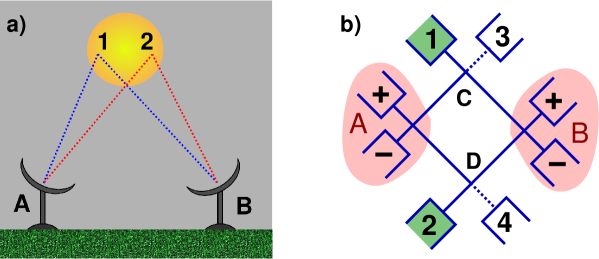
Figure 1: a) Schematic of the Hanbury Brown Twiss intensity interferometer used to measure the angular diameter of stars. Two uncorrelated points 1,2 on the star act as sources. The signal is detected at A and B. b) Schematic of the topologically equivalent two-particle interferometer (2PI) [3] with beam splitters C,D and biased, active (grounded, inactive) source contacts 1,2 (3,4). Detector regions A and B (red shaded) contain beam splitters and grounded contacts $\pm$.

To obtain a qualitative understanding of the physics of two-particle interferometers it is rewarding to compare the properties of optical, bosonic interferometers and electronic, fermionic interferometers. In Fig. 1 a schematic of a two-particle interferometer, topologically equivalent to the HBT-interferometer, is shown. A natural measure of the correlations between the particles at $A$ and $B$ is the probability to jointly detect one particle at $A$ and one at $B$. An expression for this joint detection probability for photons was derived by Glauber [44]. In Ref. [3] this was adapted to detection of electrons. Here we consider the probability to detect one photon/electron in detector $A\alpha$, $\alpha=\pm$, at time $t$ and one in detector $B\beta$, $\beta=\pm$ at a time $t+\tau$, given by

$$P_{A\alpha B\beta}(\tau)\propto\langle b^{\dagger}_{B\beta}(t)b^{\dagger}_{A\alpha}(t+\tau)b_{A\alpha}(t+\tau)b_{B\beta}(t)\rangle$$ (2)

The photon/electron creation operators at A are $b^{\dagger}_{A\alpha}(t)=\int dE~{}\mbox{exp}(iEt/\hbar)b_{A\alpha}^{\dagger}(E)$, with $b_{A\alpha}^{\dagger}(E)$ creating a particle in $A\alpha$ at energy $E$ and similarly at B. For photons we consider thermal sources in $1$ and $2$ while $3$ and $4$ are left empty. A detector frequency window of size $\Delta\omega$ is assumed, over which the distribution functions of the sources are constant, i.e. $\Delta\omega\ll kT$. For electrons we assume zero temperature and the sources $1$ and $2$ biased at $eV$ while sources $3$ and $4$ are grounded. Only quasiparticle excitations, $E\geq 0$ are considered.

The probabilities are normalized such that $\sum_{\alpha,\beta=\pm}P_{A\alpha B\beta}=1$. Following the scattering theory for intensity/current correlations for bosons/fermions emitted from thermal sources [45, 46], we get

$$P_{A\alpha B\beta}(\tau) \propto |s_{A\alpha 1}|^{2}|s_{B\beta 1}|^{2}\left[1\pm g(\tau)\right]+|s_{A\alpha 2}|^{2}|s_{B\beta 2}|^{2}\left[1\pm g(\tau)\right]$$ (3)

$$+ |s_{A\alpha 1}|^{2}|s_{B\beta 2}|^{2}+|s_{A\alpha 2}|^{2}|s_{B\beta 1}|^{2}$$

$$\pm g(\tau)\left[s_{A\alpha 1}^{*}s_{B\beta 2}^{*}s_{B\beta 1}s_{A\alpha 2}+s_{A\alpha 1}s_{B\beta 2}s_{B\beta 1}^{*}s_{A\alpha 2}^{*}\right]$$

where $g(\tau)=\sin^{2}(\tau/\pi\tau_{C})/(\tau/\pi\tau_{C})^{2}$ contains the time dependence, with $\tau_{C}=h/eV$ the coherence time for electrons and $2/\pi\Delta\omega$ for photons. Here $s_{A\alpha 2}$ is the amplitude to scatter from source 2 to detector $A\alpha$ etc. The upper/lower signs $\pm$ correspond to electrons/photons.

Several interesting conclusions can be drawn directly from Eq. (3):

1) For $\tau\gg\tau_{C}$, $g(\tau)$ approaches zero and $P_{A\alpha B\beta}$ is just proportional to the product of the two mean currents/intensities. The fermionic versus bosonic statistics of the particle plays no role.

2) For shorter times, $\tau\leq\tau_{C}$, $g(\tau)$ is finite and the statistics is important. Note that, as pointed out above, that the statistics of the particles enter in two different ways.
i) The first two terms in Eq. (3) describe a direct bunching (+) or anti-bunching (-) effect for two particles emitted from the same reservoir within a time $\tau\leq\tau_{C}$. This effect would still be present if one of the sources $1$ or $2$ is removed.
ii) The last two terms describe the two-particle, or exchange [45, 46], interference, where the $\pm$ sign explicitly follows from the interchange of the two detected particles. This two particle interference is only present when both sources are active.

For semitransparent beam-splitters $A,B,C$ and $D$ and coincident detection $\tau\ll\tau_{C}$ we have

$$P_{A\alpha B\beta}=\left\{\begin{array}[]{cc}\frac{1}{4}\left[1+\alpha\beta\cos\phi\right]&\mbox{fermions}\\ \frac{1}{4}\left[1+\frac{\alpha\beta}{2}\cos\phi\right]&\mbox{bosons}\end{array}\right.$$ (6)

where $\phi$ is a scattering phase. From this expression a very important difference between bosonic and fermionic thermal sources is apparent: the visibility

$$\nu=\frac{P_{A\alpha B\beta}^{max}-P_{A\alpha B\beta}^{min}}{P_{A\alpha B\beta}^{max}+P_{A\alpha B\beta}^{min}}$$ (7)

of the oscillations is $1$ for fermions but only $1/2$ for bosons. This is directly related to the fact that while the emitted fermionic two-particle state is maximally entangled, the bosonic state is unentangled [49].

3 Fermionic two particle interferometer: theory

In Ref. [3] we proposed an implementation of an electronic 2PI in a conductor in the quantum Hall regime, with electrons propagating along single, spin polarized edge states (see Fig. 2). Two electronic reservoirs $1,2$ biased at $eV$ act as sources for electrons while the reservoirs $3,4$ as well as the detector reservoirs are grounded. All reservoirs are kept at the same temperature $T$. Moreover, we consider here only the linear regime in voltage where electron-electron interactions can be neglected. This regime is relevant for the experiment [23]. The QPC’s at $A,B,C$ and $D$ act as beamsplitters with transparencies $T_{A},T_{B},T_{C}$ and $T_{D}$ respectively.

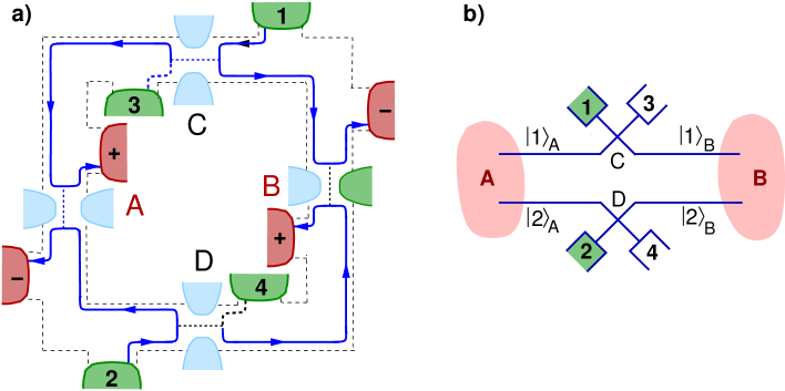
Figure 2: a) Fermionic 2PI implemented in a conductor in the quantum Hall regime, from [3]. See text for details. b) Schematic of the source part of the 2PI, with the the orbital states $|1\rangle_{A},|2\rangle_{A},|1\rangle_{B}$ and $|2\rangle_{B}$ for particles emitted out from the source towards the detectors are shown.

The scattering amplitude $s_{A+1}=\sqrt{T_{A}R_{C}}e^{i\phi_{AC}}$, where $R_{C}=1-T_{C}$ and $\phi_{AC}$ is the scattering phase picked up by the electron up when traveling from C to A. Similar relations hold for the other scattering amplitudes. Note that the total phase $\phi=\phi_{AC}-\phi_{AD}+\phi_{BD}-\phi_{BC}$ is, up to a constant term, given by $2\pi\Phi/\Phi_{0}$ where $\Phi$ is the magnetic flux threading the 2PI and $\Phi_{0}=h/e$, the single particle flux quanta. Importantly, the Corbino geometry in Fig. 2 with unidirectional edge states and reflectionless beam-splitters is topologically equivalent to the 2PI shown in Fig. 1.

3.1 Two particle Aharonov-Bohm effect

The standard tools for investigating transport properties in mesoscopic electronic systems are average electrical current and current correlation measurements [47]. A scattering theory calculation [48] gives the average current at contact $A\alpha$

$$I_{A\alpha} = \frac{e}{h}\int dE\left(|s_{A\alpha 1}|^{2}+|s_{A\alpha 2}|^{2}\right)\left[f_{V}(E)-f(E)\right]$$

and similar at $B\beta$. Here $f_{V}=1/(1+e^{(E-eV)/kT})$ and $f=1/(1+e^{E/kT})$ are the Fermi distributions of the biased, $1,2$ and the grounded, $3,4$ reservoirs respectively. The irreducible zero frequency correlator

$$S_{A\alpha B\beta}=\int dt\langle\Delta I_{A\alpha}(0)\Delta I_{B\beta}(t)\rangle$$ (9)

between currents $I_{A\alpha}(t)=I_{A\alpha}+\Delta I_{A\alpha}(t)$ and $I_{B\beta}(t)=I_{B\beta}+\Delta I_{B\beta}(t)$ [46] becomes

$$S_{A\alpha B\beta}=\frac{e^{2}V}{h}\int dE\left(|s_{A\alpha 1}^{*}s_{B\beta 1}+s_{A\alpha 2}^{*}s_{B\beta 2}|^{2}\right)\left[f_{V}(E)-f(E)\right]^{2}$$ (10)

These expressions are valid for arbitrary temperature but for the rest of the discussion in this section we only consider the zero temperature case. In particular, for the simplest possible case, with all beam-splitters semitransparent and energy-independent scattering amplitudes, we have

$$I_{A\alpha}=I_{B\beta}=\frac{e^{2}V}{2h},\hskip 14.22636ptS_{A\alpha B\beta}=\frac{e^{3}V}{4h}\left[1+\alpha\beta\cos\phi\right]$$ (11)

While the average current is a function of QPC-transparencies only, the current cross correlator depends also on the phase $\phi$. Since this phase is proportional to the magnetic flux $\Phi$ threading the 2PI, we call this a two-particle Aharonov-Bohm (AB) effect.

Interestingly, we can directly relate the coincident detection probability in Eq. (3) at times $\tau\ll\tau_{C}$ with the currents in Eq. (LABEL:curr) and the zero frequency noise correlators in Eq. (10) as $[g(0)=1]$

$$P_{A\alpha B\beta}(0) \propto |s_{A\alpha 1}s_{B\beta 1}^{*}+s_{A\alpha 2}s_{B\beta 2}^{*}|^{2}+\left(|s_{A\alpha 1}|^{2}+|s_{A\alpha 2}|^{2}\right)\left(|s_{B\beta 1}|^{2}+|s_{B\beta 2}|^{2}\right)$$ (12)

$$\propto S_{A\alpha B\beta}+2\tau_{C}I_{A\alpha}I_{B\beta}$$

This is a direct consequence of fermionic anti-bunching, leading to a filled stream of electrons emitted from the source reservoirs and hence making long time observables an effective average of many individual, short time, single and two-particle events.

3.2 Entanglement

The connection between this two-particle Aharonov-Bohm effect and entanglement can be seen by considering the many-body ground state $|\Psi_{in}\rangle$ of the electrons injected into the 2PI. Electrons at different energies are independent and the many-body state at zero temperature is thus a product state in energy

$$|\Psi_{in}\rangle=\prod_{0\leq E\leq eV}a_{1}^{\dagger}(E)a_{2}^{\dagger}(E)|\bar{0}\rangle$$ (13)

where $|\bar{0}\rangle$ is the filled Fermi sea and $a^{\dagger}_{1}(E)$ creates an electron at energy $E$, incident from reservoir $1$. Adopting the formalism of Ref. [2] we first define $|\Psi_{in}(E)\rangle=a_{1}^{\dagger}(E)a_{2}^{\dagger}(E)|\bar{0}\rangle$ the injected state at energy $E$. We have the scattering relations at the two source beam splitters, suppressing energy notation

$$\left(\begin{array}[]{c}b_{A1}\\ b_{B1}\end{array}\right)=\left(\begin{array}[]{cc}r_{C}&t_{C}^{\prime}\\ t_{C}&r_{C}^{\prime}\end{array}\right)\left(\begin{array}[]{c}a_{1}\\ a_{3}\end{array}\right),\hskip 14.22636pt\left(\begin{array}[]{c}b_{A2}\\ b_{B2}\end{array}\right)=\left(\begin{array}[]{cc}r_{D}&t_{D}^{\prime}\\ t_{D}&r_{D}^{\prime}\end{array}\right)\left(\begin{array}[]{c}a_{2}\\ a_{4}\end{array}\ \right)$$ (14)

for incoming (a’s) and outgoing (b’s) electrons. The primed scattering amplitudes thus describes particles incoming from the unbiased sources. This gives the emitted state for the electrons at energy $E$, after beam-splitters $C,D$ but before impinging on the detector beam splitters $A,B$, as

$$|\Psi_{out}(E)\rangle=\left(r_{C}b_{A1}^{\dagger}+t_{C}b_{B1}^{\dagger}\right)\left(r_{D}b_{A2}^{\dagger}+t_{D}b_{B2}^{\dagger}\right)|\bar{0}\rangle$$ (15)

Since we are interested in entanglement between particles in the two, spatially separated detector regions A and B we project out the part of the wave function with one particle in A and one in B yielding the normalized wavefunction

$$|\Psi_{AB}(E)\rangle=\frac{1}{\sqrt{N}}\left(r_{C}t_{D}b_{A1}^{\dagger}b_{B2}^{\dagger}-r_{D}t_{C}b_{A2}^{\dagger}b_{B1}^{\dagger}\right)|\bar{0}\rangle$$ (16)

with $N=|r_{D}t_{C}|^{2}+|r_{C}t_{D}|^{2}=R_{C}T_{D}+R_{D}T_{C}$ the normalization constant. Here we introduced the transmission and reflection probabilities of the source beam splitters as $T_{C}=|t_{C}|^{2}=|t_{C}^{\prime}|^{2}$ and $R_{C}=|r_{C}|^{2}=|r_{C}^{\prime}|^{2}=1-T_{C}$ for C and similarly for D. To make this more transparent we can, since the two particles live in well separated Hilbert spaces, introduce the Dirac notation $|1\rangle_{A}\equiv b_{A1}^{\dagger}|\bar{0}\rangle$ etc, and write

$$|\Psi_{AB}(E)\rangle=\frac{1}{\sqrt{N}}\left[r_{C}t_{D}|1\rangle_{A}|2\rangle_{B}-t_{C}r_{C}|2\rangle_{A}|1\rangle_{B}\right]$$ (17)

which for semi-transparent beam splitters (and scattering phase $\phi=0$) reduces to the singlet state $|\Psi_{s}\rangle$ in Eq. (1). The orbital states are shown in Fig. 2

The entanglement of the state $|\Psi_{AB}(E)\rangle$ can conveniently be quantified in terms of the concurrence $C$ [50], which ranges from zero for an unentangled state to unity for a maximally entangled state. Working in the computational basis $\{|1\rangle_{A}|1\rangle_{B},|1\rangle_{A}|2\rangle_{B},|2\rangle_{A}|1\rangle_{B},|2\rangle_{A}|2\rangle_{B}\}$, for the pure state $|\Psi_{AB}\rangle$ in Eq. (17) we have

$$C=|\langle\Psi_{AB}|(\sigma_{y}\otimes\sigma_{y})|\Psi_{AB}^{*}\rangle|$$ (18)

where $|\Psi_{AB}^{*}\rangle$ is $|\Psi_{AB}\rangle$ with all coefficients complex conjugated, $\sigma_{y}$ a Pauli matrix and $\otimes$ the direct, tensor product. We thus find for $|\Psi_{AB}\rangle$ the concurrence

$$C=\frac{2}{N}|r_{C}t_{C}r_{D}t_{D}|=\frac{2}{N}\sqrt{R_{C}T_{C}R_{D}T_{D}}$$ (19)

which reaches unity for semitransparent beam splitters, i.e. for the singlet state in Eq. (1). Note that the normalization factor $N$ is maximal, equal to $1/2$, for semitransparent beam splitters. This demonstrates that at most only half of the particles injected from $1$ and $2$ lead to split pairs, with one particle emitted towards $A$ and one towards $B$, i.e. a maximal pair emission rate of $1/2$. For a measurement during a time $\tau$ the maximum concurrence production [11] is thus ${\mathcal{N}}/2$, where ${\mathcal{N}}=\tau eV/h$ the number of pairs injected from $1$ and $2$ in the time $\tau$ and energy interval $0\leq E\leq eV$

3.3 Dephasing

There are several microscopic mechanisms that can lead to dephasing, typically suppressing the two-particle interference. For low temperatures it is commonly believed that the dominatinating mechanism for dephasing is electron-electron interactions, but this is still a topic of ongoing research and goes beyond the scope of the present work. Here we consider no specific mechanism but model dephasing qualitatively by coupling one of the interferometer arms to a dephasing voltage probe [51, 52, 53, 54]. In this context we point out a recent experiment [55]: a voltage probe was coupled, via a tunable quantum point contact, to one arm of a Mach Zehnder interferometer in the quantum Hall regime, demonstrating controllable dephasing. Considering semitransparent beam splitters, the dephasing probe coupled with a strength $0\leq\gamma\leq 1$ lead to a modification of the current correlator in Eq. (11) to [56]

$$S_{A\alpha B\beta}^{deph}=\frac{e^{3}V}{4h}\left[1+\gamma\alpha\beta\cos\phi\right]$$ (20)

From this expression it is clear that $\gamma$ enters as a decoherence parameter; decreasing $\gamma$ from $1$ to $0$ leads to a suppression the phase dependence of the current correlator. In the presence of dephasing the emitted state is no longer a pure state, it is instead a mixed state described by a density matrix $\sigma_{AB}$. Considering zero temperature, working in the computational basis the result for $S_{A\alpha B\beta}^{deph}$ corresponds to a suppression of the off-diagonal components of $|\Psi_{AB}\rangle\langle\Psi_{AB}|\rightarrow\sigma_{AB}$ as

$$\sigma_{AB}=\frac{1}{2}\left(\begin{array}[]{cccc}0&0&0&0\\ 0&1&-\gamma&0\\ 0&-\gamma&1&0\\ 0&0&0&0\end{array}\right)$$ (21)

The concurrence for a mixed state is [50]

$$C=\mbox{max}\left\{\sqrt{\lambda_{1}}-\sqrt{\lambda_{2}}-\sqrt{\lambda_{3}}-\sqrt{\lambda_{4}},0\right\}$$ (22)

where $\lambda_{i}$, $i=1-4$, are the eigenvalues in decreasing order of $\sigma_{AB}(\sigma_{y}\otimes\sigma_{y})\sigma^{*}_{AB}(\sigma_{y}\otimes\sigma_{y})$. We then have

$$C=\gamma$$ (23)

This means that the entanglement persists even for very strong dephasing [31, 32, 33]. This is a consequence of the 2PI-geometry, where scattering between the arms, i.e. pseudo spin-flip scattering, is prohibited.

3.4 Fermionic two particle interferometer: experiment

Very recently the electronic 2PI was realized experimentally by Neder et al. In the experiment, in the quantum Hall regime, it was possible to electrically tune the system between two individual Mach Zehnder interferometers and a 2PI, as shown schematically in fig. 3.

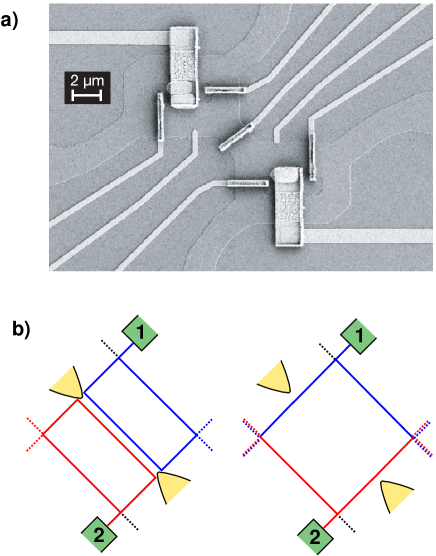
Figure 3: Fermionic two-particle interferometer implemented in a conductor in the quantum Hall regime in Ref [23]. a) Figure reproduced from Ref. [23]. Micrograph of the sample. b) Left: The system in the two Mach Zehnder interferometers configuration. Right: The system in the 2PI configuration.

The authors first tuned the system to two Mach-Zehnder interferometers and measured the single particle interference in the average current for each interferometer. They found a very large visibility in both interferometers, around $80\%$. They also determined the periods of the single particle AB-oscillations as a function of both the area and the magnetic flux enclosed by the interferometers. Thereafter the system was tuned to a single 2PI. As predicted by theory [3] no single-particle AB-oscillations in the average current were observed but the current cross correlations displayed clear two-particle AB-oscillations, with an amplitude $25\%$ of the predicted coherent, zero temperature value. By measuring also the period of the two-particle oscillations as a function of interferometer area and enclosed flux and comparing to the sum of the periods for the two Mach Zehnder interferometers, the two-particle nature of the AB-oscillations could be established beyond doubt.

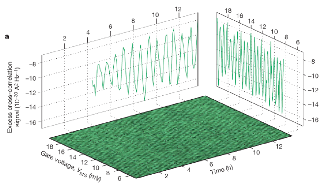
Figure 4: Figure reproduced from Ref. [23]. Experimental demonstration of the two-particle AB-effect. Current cross correlation displaying clear oscillations as a function of the effective interferometer area and enclosed magnetic flux.

In the experiment semitransparent beam splitters were used, $T_{C}=T_{D}=1/2$. For the current cross correlations, theory for finite temperature and dephasing [56] predicts, for $A+,B+$,

$$S_{A+B+}=-\frac{e^{3}V}{4h}H\left[1-\gamma\sin\phi\right].$$ (24)

The temperature dependence is fully contained in

$$H=\coth\left(\frac{eV}{2kT}\right)-\frac{2kT}{eV},$$ (25)

varying from unity for $kT\ll eV$ to zero for $kT\gg eV$. The effect of finite temperature is thus to suppress the overall amplitude of the current cross correlation oscillations. In the experiment, the applied bias was $7.8\mu V$. The electron temperature was estimated from independent auto-correlation measurements to be $10mK$. This yields the temperature suppression factor $H=0.78$. A direct comparison to Eq. (24) then gives the oscillation amplitude $H\gamma=0.25$, i.e. $\gamma=0.32$, a substantial dephasing.

4 Finite temperature state

Our main aim of this work is to theoretically investigate the effects of finite temperature on the entanglement of the state emitted out from the source, towards the detectors. A prerequisite is to obtain both a qualitative and a quantitative description of the emitted many-body state at finite temperature. We consider the experimentally relevant situation with all source and detector reservoirs kept at the same temperature $T$. Due to the finite temperature, not only the electrons emitted from the source in the energy range $0\leq E\leq eV$ are of interest, we must in principle take into account particles emitted from all reservoirs at all possible energies. However, due to the chiral geometry of the 2PI in Fig. 2, particles emitted from the detectors can never scatter back to the detectors, i.e. detector cross talk is topologically prohibited. The particles arriving at the detectors thus all originate from the source reservoirs and we can focus on the many body state emitted by source $1$ to $4$. We note that in the slightly different geometry realized experimentally [23], there is the possibility for scattering between the detectors. It can however be shown [57] that this does not influence the entanglement of the emitted state.

At finite temperature the state injected from the sources is mixed and described by a density matrix [11]

$$\rho_{in} = \prod_{E}\rho_{in}(E)$$

$$\rho_{in}(E) = \prod_{\kappa=1}^{4}\left[[1-f_{\kappa}(E)]|0\rangle\langle 0|+f_{\kappa}(E)a^{\dagger}_{\kappa}(E)|0\rangle\langle 0|a_{\kappa}(E)\right]$$ (26)

where $f_{\kappa}(E)$ is the Fermi distribution of source reservoir $\kappa=1-4$. The outgoing state is then obtained by inserting the scattering relations of Eq. (14) int Eq. (26).

One can see from Eq. (26) that the effect of finite temperature is to give rise to states with 0 to 4 particles emitted at a given energy. For the terms of interest, i.e. with at least one particle at both A and B, there is at finite temperature the possibility for e.g. two particles at A and one at B etc. These terms are of central importance in the discussion below.

5 Projected two-particle density matrix

A theory for entanglement production in non-interacting [2] conductors at finite temperature was presented by Beenakker [11] and along similar lines in closed condensed matter systems by Dowling, Doherty and Wiseman [58]. At a given energy, only the component of the emitted many-body state with one particle in detector region A and one in B has nonzero entanglement. Moreover, as emphasized in Ref. [58], only this term describes two particles which each live in a well defined $2\times 2$ Hilbert spaces at A and B respectively, i.e. two coupled orbital qubits. We point out that this definition does not take into account occupation-number, or Fock-space entanglement. The first step is thus to project out the two-particle component from the many-body wave function, which is accomplished by the projection operator

$$\Pi=\Pi_{A}\otimes\Pi_{B},\hskip 14.22636pt\Pi_{\alpha}=n_{\alpha 1}(1-n_{\alpha 2})+n_{\alpha 2}(1-n_{\alpha 1})$$ (27)

where $n_{Aj}=b_{Aj}^{\dagger}b_{Aj}$ with $j=1,2$ etc is the number operator (suppressing energy notation). This yields the projected density matrix

$$\rho_{p}(E)=\Pi\rho(E)\Pi$$ (28)

The elements of the density matrix $\rho_{p}(E)$ are conveniently calculated from the relation [58]

$$[\rho_{p}(E)]_{ij,kl}=\langle\Pi b_{Ai}^{\dagger}b_{Bj}^{\dagger}b_{Bk}b_{Al}\Pi\rangle$$ (29)

where, for any operator X, $\langle X\rangle=\mbox{tr}[X\rho]$ is the standard quantum-statistical average. Some algebra gives the projected density matrix, formally equivalent to the density matrix calculated in [11], Eqs. (B9) - (B13),

$$\rho_{p}(E)=(1-f)^{2}f_{V}^{2}\left(\begin{array}[]{cccc}\chi&0&0&0\\ 0&c_{12}^{12}&c_{12}^{21}&0\\ 0&c_{21}^{12}&c_{21}^{21}&0\\ 0&0&0&\chi\end{array}\right)$$ (30)

where $\chi=e^{-eV/kT}$ and $f$ and $f_{V}$ the Fermi distribution functions of the grounded and biased source reservoirs respectively. The coefficients

$$c_{12}^{12} = (R_{C}[1-\chi]+\chi)(T_{D}[1-\chi]+\chi),$$

$$c_{21}^{21} = (T_{C}[1-\chi]+\chi)(R_{D}[1-\chi]+\chi),$$

$$c_{12}^{21} = (c_{21}^{12})^{*}=-\gamma\sqrt{R_{C}T_{C}R_{D}T_{D}}e^{i\phi_{0}}(1-\chi)^{2}$$ (31)

with $\phi_{0}$ an overall scattering phase of the beam splitters C and D. Thus, only the prefactor $f_{V}^{2}(1-f)^{2}$ depends on energy. As for the zero temperature case we have introduced dephasing as a suppression of the off-diagonal components of the density matrix. It follows from Eq. (30) that finite temperature leads to
i) an overall modification of the energy-dependent probability for two-particle emission via the prefactor $(1-f)^{2}f_{V}^{2}$.
ii) a suppression $\sim(1-\chi)^{2}$ of the off-diagonal components, equivalent to the effect of dephasing.
iii) a finite amplitude for the diagonal density matrix elements $[\rho_{p}(E)]_{11,11}$ and $[\rho_{p}(E)]_{22,22}$, i.e for two particles being emitted from either sources 1,3 or 2,4.

Additional insight follows from writing the projected density matrix as

$$\rho_{p}(E)=(1-f)^{2}f_{V}^{2}\left[\chi\rho_{p}^{diag}+(1-\chi)^{2}\rho^{int}\right]$$ (32)

where the diagonal density matrix

$$\rho_{p}^{diag}=\chi\hat{1}\otimes\hat{1}+(1-\chi)[\rho_{A}\otimes\hat{1}+\hat{1}\otimes\rho_{B}]$$ (33)

with the zero temperature single particle density matrices $\rho_{A}=R_{C}|1\rangle\langle 1|+R_{D}|2\rangle\langle 2|$ and $\rho_{B}=T_{C}|1\rangle\langle 1|+T_{D}|2\rangle\langle 2|$. The density matrix

$$\rho^{int} = R_{C}T_{D}|12\rangle\langle 21|+R_{D}T_{C}|21\rangle\langle 12|$$ (34)

$$- \gamma\sqrt{T_{C}R_{C}T_{D}R_{D}}[e^{i\phi_{0}}|21\rangle\langle 21|+e^{-i\phi_{0}}|12\rangle\langle 12|]$$

results from the two-particle interference. Here we used the shorthand notation $|12\rangle\equiv|1\rangle_{A}|2\rangle_{B}$ with $\langle 21|=(|12\rangle)^{\dagger}$ etc. Note that the effect of decoherence enters as a suppression of the two-particle interference $|\Psi^{int}\rangle\langle\Psi^{int}|\rightarrow\rho^{int}$, where $|\Psi^{int}\rangle=\sqrt{R_{C}T_{D}}|12\rangle-e^{i\phi_{0}}\sqrt{T_{C}R_{D}}|21\rangle$.

Writing $\rho_{p}(E)$ in the form in Eq. (32) shows that, taken the energy dependent prefactor $f_{V}^{2}(1-f)^{2}$ aside, the effects of finite temperature can be viewed as follows: First, the amplitude of the two-particle interference component $\rho^{int}$ is suppressed with increasing temperature as $\sim(1-\chi)^{2}$. Second, the density matrix acquires a purely diagonal component $\rho_{p}^{diag}$ with an amplitude $\sim\chi$ (note that $\mbox{tr}[\rho_{p}^{diag}]=4$, independent on temperature).

For the entanglement, following [11] we introduce $\sigma_{p}$ and $w_{p}(E)$, the normalized density matrix and the emission probability of the emitted two-particle state respectively, defined from

$$\rho_{p}(E) = w_{p}(E)\sigma_{p},$$

$$w_{p}(E) = \mbox{tr}[\rho_{p}(E)]=(1-f)^{2}f_{V}^{2}[(R_{C}T_{D}+T_{C}R_{D})(1-\chi)^{2}+4\chi]$$ (35)

where we note that $\sigma_{p}$ is independent on energy. The emission probability $w_{p}(E)$ is thus the probability, per unit energy, that the (normalized) two-particle state $\sigma_{p}$ is emitted. The concurrence production per unit energy is then

$$C_{p}(E) \equiv w_{p}(E)C(\sigma_{p})=\frac{(1-\chi)^{2}f_{V}^{2}(1-f)^{2}}{2}$$ (36)

$$\times \mbox{max}\left\{4\gamma\sqrt{R_{C}T_{C}R_{D}T_{D}}-\frac{1}{\sinh^{2}(eV/2kT)},0\right\}$$

and the total entanglement production during a time $\tau$, $C_{p}=(\tau/h)\int dEC_{p}(E)$, is then (${\mathcal{N}}=\tau eV/h$)

$$C_{p}=\frac{{\mathcal{N}}H}{2}\mbox{max}\left\{4\gamma\sqrt{T_{C}R_{C}T_{D}R_{D}}-\frac{1}{\sinh^{2}(eV/2kT)},0\right\}.$$ (37)

We denote this the projected entanglement. As shown in Fig. 5, $C_{p}$ decreases monotonically as a function of $T$. It reaches zero at a critical temperature $T_{c}^{p}$ given by

$$kT_{c}^{p}=eV\ln\left(\frac{\sqrt{1+4\gamma\sqrt{R_{C}T_{C}R_{D}T_{D}}}+1}{\sqrt{1+4\gamma\sqrt{R_{C}T_{C}R_{D}T_{D}}}-1}\right)$$ (38)

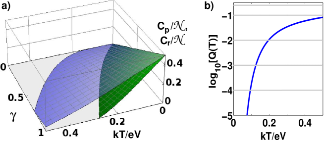
Figure 5: a) Entanglement production $C_{p}/{\mathcal{N}}$ (blue, transparent) and $C_{r}/{\mathcal{N}}$ (green, opaque) as functions of temperature $kT/eV$ and coherence $\gamma$ for the semi-transparent 2PI. b) Parameter $Q$ as a function of $kT/eV$ (blue line). Values $0.25,10^{-1},10^{-2},10^{-3},10^{-4}$ shown (gray lines). Figure reproduced from Ref. [34].

For semi-transparent beam-splitters and zero dephasing, $\gamma=1$, the entanglement thus survives up to [11] $kT_{c}^{p}=0.57eV$.

Inserting the parameter values from the experiment, we get $C_{p}\approx 0.1{\mathcal{N}}$ and $C(\sigma_{p})\approx 0.3$, i.e. the state emitted by the 2PI is clearly entangled. Importantly, the effect of finite temperature is essentially negligible, the reduction in entanglement comes from decoherence.

The entanglement of the projected density matrix is the entanglement one could access, had one been able to do arbitrary local operations and classical communication between A and B, i.e. fully energy and particle resolved measurements. Under realistic conditions this is not possible, the accessible physical quantities are currents and current cross correlators. Is it possible to determine the projected entanglement with such measurements? The answer to this question is no, for two main reasons:
i) As discussed above, at nonzero temperatures it is not only the biased source reservoirs which emit particles but also the grounded source reservoirs do. As a consequence, there is a finite amplitude for emitted states with two-particles at A and/or at B. These unentangled states contribute to currents and current correlators, which results in a detectable state with suppressed entanglement.
ii) The current and current correlators provide information on the energy integrated properties of the many-body state, not on the emitted state at each energy. This lack of energy-resolved information leads to a further suppression of the detectable entanglement.
Clearly, these effects of the thermally excited Fermi sea constitute generic problems when trying to detect entanglement in mesoscopic conductors.

As a remedy for these finite temperature read-out problems it was suggested to work with detectors at very low temperatures [11]. Another idea was recently presented by Hannes and Titov [8]. They investigated detection of entanglement at finite temperatures via a Bell inequality and proposed to introduce energy filters at the drains. However, both schemes [11, 8] would lead to additional experimental complications in systems which already are experimentally very challenging. Our idea is instead to investigate what information about the projected entanglement can actually be deduced from current and current correlation measurements.

In this context we also mention the recent proposal by Kindermann [9], to produce and detect entangled electron-hole pairs in graphene via a Bell inequality formulated in terms of the transport part of the current cross correlators [46], i.e. by subtracting away the thermal equilibrium correlators from the finite bias ones. In our work [34] we proposed a similar scheme for a general mesoscopic conductor. However, as was pointed out in [34] and is further discussed below, it is important that one performs a detailed comparison of the projected entanglement and the entanglement obtained from current cross correlation measurements. Without such a comparison, there is the possibility that one concludes, based on correlation measurements, finite entanglement where there is none, i.e. the projected entanglement is zero.

6 Reduced two-particle density matrix

We first consider the expression for the current and zero frequency current cross correlators at contacts $A+$ and $B+$ at finite temperatures. We have

$$I_{A+} = \frac{e}{h}\int dE\left[\langle n_{A+}\rangle-f\right],\hskip 14.22636ptI_{B+}=\frac{e}{h}\int dE\left[\langle n_{B+}\rangle-f\right],$$

$$S_{A+B+} = \frac{e^{2}}{h}\int dE\langle\Delta n_{A+}\Delta n_{B+}\rangle$$ (39)

where $\langle\Delta n_{A+}\Delta n_{B+}\rangle=\langle n_{A+}n_{B+}\rangle-\langle n_{A+}\rangle\langle n_{B+}\rangle$ is the irreducible correlator. As discussed above, the many-body state incident on the detectors originates from the sources. It is the properties of this state that determines the observables $\langle n_{A+}\rangle,\langle n_{B+}\rangle$ and $\langle\Delta n_{A+}\Delta n_{B+}\rangle$ and thus establishes a connection between the emitted state and the physical quantities accessible in a measurement.

6.1 Energy resolved reduced density matrix

In order to better understand the readout problem discussed above, we first discuss the energy resolved properties of the emitted state. If one would have access to energy filters, as proposed in [8], or would be working at zero temperature, by combining current and current cross correlations it would be possible to get direct access to the energy resolved quantities $\langle n_{A+}\rangle,\langle n_{B+}\rangle$ and $\langle\Delta n_{A+}\Delta n_{B+}\rangle$. As is discussed below, by a suitable set of measurements with different settings of the beam splitters at A and B one could then tomographically reconstruct the (unnormalized) density matrix of the state emitted out from the source beam splitters C and D, $\rho_{r}^{E}$, with elements given by

$$[\rho_{r}^{E}]_{ij,kl}=\langle b_{Ai}^{\dagger}b_{Bj}^{\dagger}b_{Bk}b_{Al}\rangle$$ (40)

We denote $\rho_{r}^{E}$ the energy resolved reduced density matrix.

By comparing $\rho_{r}^{E}$ with the expression for the projected density matrix in Eq. (30) we see that it differs by the projection operators. Consequently, the reduced density matrix contains also the contributions from processes with more than one particle at A and/or at B. After some algebra we find the density matrix

$$\rho_{r}^{E}=(1-f)^{2}f_{V}^{2}\left(\begin{array}[]{cccc}\tilde{\chi}&0&0&0\\ 0&\tilde{c}_{12}^{12}&c_{12}^{21}&0\\ 0&c_{21}^{12}&\tilde{c}_{21}^{21}&0\\ 0&0&0&\tilde{\chi}\end{array}\right)$$ (41)

where we introduced $\tilde{\chi}=\chi/[(1-f_{V})(1-f)]$ and the coefficients

$$\tilde{c}_{12}^{12} = (R_{C}[1-\chi]+\chi)(T_{D}[1-\chi]+\tilde{\chi}),$$

$$\tilde{c}_{21}^{21} = (T_{C}[1-\chi]+\chi)(R_{D}[1-\chi]+\tilde{\chi}).$$ (42)

A comparison to the projected density matrix in Eq. (30) shows that $\rho_{r}^{E}$ only differs formally from $\rho_{p}(E)$ by the change $\chi\rightarrow\tilde{\chi}$ at a number of places. This has the consequence that the normalized density matrix $\sigma_{r}^{E}=\rho_{r}^{E}/w_{r}^{E}$, with $w_{R}^{E}=\mbox{tr}[\rho_{r}^{E}]$ depend on energy. That is, in contrast to $\rho_{p}$ both the normalized, emitted two-particle state as well as the emission probability depend on energy. Qualitatively, as discussed above, the difference between $\rho_{r}^{E}$ and $\rho_{p}(E)$ arises from the fact that also states with more than one particle at A and/or B contribute to $\rho_{r}^{E}$ but not to $\rho_{p}(E)$. Writing $\rho_{r}^{E}$ on a form similar to Eq. (32) one sees that these three and four particle states contribute only to the diagonal part of $\rho_{r}^{E}$.

Turning to the entanglement, the concurrence production $C_{r}^{E}=w_{r}^{E}C(\sigma_{r}^{E})$ at energy $E$ is then

$$C_{r}^{E} = \frac{(1-\chi)^{2}f_{V}^{2}(1-f)^{2}}{2}$$ (43)

$$\times \mbox{max}\left\{4\gamma\sqrt{R_{C}T_{C}R_{D}T_{D}}-\frac{1}{\sinh^{2}(eV/2kT)}\frac{1}{(1-f_{V})(1-f)},0\right\}$$

From the expression for the concurrence it becomes clear that the separable three and four-particle states are detrimental for the entanglement. Hence, finite temperature leads to a stronger suppression of the reduced, energy resolved density matrix than of the projected one. This is illustrated in fig. 6 where the corresponding concurrencies are plotted for semitransparent beam-splitters and different values of $kT/eV$.

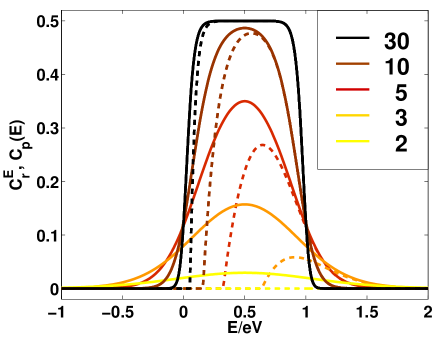
Figure 6: A comparison of the concurrence production rates $C_{r}^{E}$ (dashed) and $C_{p}(E)$ (solid), as a function of energy for $T_{C}=T_{D}=1/2$ and different ratios $eV/kT$.

As is clear from the figure, there is an energy $E_{0}$ above which the concurrence is finite (up to $E\rightarrow\infty$). The energy $E_{0}$ is given by the condition $C_{r}^{E}(E_{0})=0$, as

$$E_{0}=kT\left(\ln[2]-\ln\left[(1-\chi)\sqrt{1+4\sqrt{R_{C}T_{C}R_{D}T_{D}}}-(1+\chi)\right]\right)$$ (44)

What is moreover clear from Fig. 6 is that, for all energies, $C_{r}^{E}(E)<C_{p}(E)$. The difference is obvious for energies $E<E_{0}$, where $C_{r}^{E}=0$. At these energies the probability for emission of separable three and four particle states is thus large enough to completely suppress the entanglement of the reduced density matrix.

Importantly, the relation $C_{r}^{E}(E)<C_{p}(E)$ holds for all settings of the beam splitters $T_{C}$ and $T_{D}$, as is clear by comparing Eqs. (36) and (43). The reason for this is that the reduced density matrix contains contributions from all individual particle density matrices $\sigma_{ij}$ with $i,j\geq 1$ (e.g. $\sigma_{12}$ describes one particle at A and two at B) while the projected density matrix only depends on $\sigma_{11}$. Since all $\sigma_{12},\sigma_{21},\sigma_{22}$ are separable and the concurrence is a convex quantity, i.e. $C(p_{1}\sigma_{1}+p_{2}\sigma_{2})\leq p_{1}C(\sigma_{1})+p_{2}C(\sigma_{2})$ for $p_{1}+p_{2}=1$, the concurrence $C_{r}^{E}$ is always smaller than $C_{p}(E)$. We point out that this carries over to the total concurrence production found by integrating Eq. (43) over energy (result not presented here).

It follows from Eq. (44) that for a critical temperature $T_{c}^{rE}$ the energy $E_{0}\rightarrow\infty$, i.e. the entanglement is zero for any energy. Interestingly, this happens for the same temperature as for the projected concurrence, Eq. (38).

6.2 Finite temperature reduced density matrix

Importantly, at finite temperature, without any energy filters, we do not have access to the energy resolved quantities discussed above, only to the total currents and current correlators measured at contacts $A\alpha,B\beta$. In Ref. [35] it was discussed how to, at zero temperature, tomographically reconstruct the reduced density matrix using currents and current correlations. Extending this scheme to nonzero temperatures it is natural to define the finite temperature reduced density matrix $\rho_{r}$ via the relation

$$\frac{I_{A\alpha}I_{B\beta}}{(Ve^{2}/h)^{2}}+\frac{S_{A\alpha B\beta}}{2Ve^{3}/h}=\mbox{tr}\left\{\left[I_{A\alpha}^{O}\otimes I_{B\beta}^{O}\right]\rho_{r}\right\}.$$ (45)

We emphasize that $\rho_{r}$ is reconstructed from observables already integrated over energy and does hence not depend on energy. Also note that $\rho_{r}$ is not given by integrating $\rho_{r}^{E}$ over energy, in fact the difference between the two density matrices is further discussed below.

In Eq. 45 the orbital current operators in the local basis $\{|1\rangle,|2\rangle\}$, including the rotations at the detector splitters, are $I_{A\alpha}^{O}=(\hat{1}+\alpha{\mathbf{n}}_{A}\cdot\hat{\sigma})/2$ and $I_{B\beta}^{O}=(\hat{1}+\beta{\mathbf{n}}_{B}\cdot\hat{\sigma})/2$, with ${\mathbf{n}}_{A}\cdot\hat{\sigma}=S_{A}\sigma_{z}S_{A}^{\dagger}$ and ${\mathbf{n}}_{B}\cdot\hat{\sigma}=S_{B}\sigma_{z}S_{B}^{\dagger}$ where $\hat{\sigma}=[\sigma_{x},\sigma_{y},\sigma_{z}]$ a vector of Pauli matrices and $S_{A}~{}(S_{B})$ the scattering matrix of the beam splitter at A (B).

Making use of the results for finite temperature current and current correlations in [56] we obtain the reduced density matrix

$$\rho_{r}=\left(\begin{array}[]{cccc}R_{C}T_{C}(1-H)&0&0&0\\ 0&R_{C}T_{D}&d^{12}_{21}&0\\ 0&d_{12}^{21}&R_{D}T_{C}&0\\ 0&0&0&R_{D}T_{D}(1-H)\end{array}\right)$$ (46)

where $d^{12}_{21}=(d_{12}^{21})^{*}=-H\gamma\sqrt{R_{C}T_{C}R_{D}T_{D}}e^{i\phi_{0}}$. Comparing $\rho_{r}$ to both $\rho_{p}(E)$ and $\rho_{r}^{E}$ in Eqs. (30) and (41) it is clear that the qualitative effect of finite temperature is the same for the reduced density matrix. The quantitative effects are however different. First, the temperature dependence enters via $H$ rather than via $\chi$, giving a much stronger effect of finite temperature. This is the effect of having access to energy integrated quantities only. Second, in the expression for the average current in Eq. (39), in the integrand one subtracts $f$ which arises due to particles flowing out of the detector reservoirs. This yields smaller diagonal terms, to be further discussed below.

It is illuminating, just as for $\rho_{p}(E)$, to write $\rho_{r}$ as a sum of a diagonal and an interference part,

$$\rho_{r}=(1-H)[\rho_{A}\otimes\rho_{B}]+H\rho^{int}.$$ (47)

From this we see that the effect of increasing temperature is to monotonically increase the amplitude for the separable product state $\rho_{A}\otimes\rho_{B}$, while the amplitude of the interference component is suppressed. We can thus conclude the following properties for all three density matrices $\rho_{p}(E),\rho_{r}^{E}$ and $\rho_{r}$:
i) At zero temperature they all reduce to the same expression, $\rho^{int}$.
ii) Increasing temperature leads to a monotonic suppression of the two-particle interference component.
iii) Finite temperature introduces an additional diagonal component, different for the three density matrices.

Turning to entanglement, introducing the normalized reduced density matrix $\sigma_{r}$ we can write

$$\rho_{r} = w_{r}\sigma_{r}$$

$$w_{r} = \mbox{tr}[\rho_{r}]=[R_{C}T_{C}+R_{D}T_{D}](1-H)+R_{C}T_{D}+R_{D}T_{C}.$$ (48)

We then define the total entanglement production during a time $\tau$ as $C_{r}\equiv{\mathcal{N}}w_{r}C(\sigma_{r})$. It is

$$C_{r}=2{\mathcal{N}}\mbox{max}\{\sqrt{T_{C}R_{C}T_{D}R_{D}}[H(1+\gamma)-1],0\}$$ (49)

here called the reduced entanglement. As $C_{p}$, $C_{r}$ decreases monotonically with increasing $T$. It reaches zero at a critical temperature $T_{c}^{r}$ given by the relation

$$H(T_{c}^{r})=\frac{1}{1+\gamma}$$ (50)

For perfect coherence, $\gamma=1$, we have $kT_{c}^{r}=0.28eV$, close to one half of $kT_{c}^{p}$. Importantly, in contrast to $T_{c}^{p}$, $T_{c}^{r}$ is independent on the setting of the beam splitters.

By comparing the expressions for the two quantities of main interest, the projected and reduced concurrencies, $C_{p}$ in Eq. (37) and $C_{r}$ in Eq. (49), we can conclude the following:
i) For both $C_{p}$ and $C_{r}$ the origin of the entanglement is the two-particle interference, in fact the component $\rho^{int}$ gives rise to the positive term $2{\mathcal{N}}H\gamma\sqrt{T_{C}R_{C}T_{D}R_{D}}$, identical for $C_{p}$ and $C_{r}$.
ii) For both $C_{p}$ and $C_{r}$ finite temperature introduces a negative term, $-{\mathcal{N}}H/[2\sinh^{2}(eV/2kT)]$ for $C_{p}$ and $-2{\mathcal{N}}(1-H)\sqrt{T_{C}R_{C}T_{D}R_{D}}$ for $C_{r}$, which leads to a suppression of the concurrence. These terms arise from the separable, diagonal components of the corresponding density matrices.

7 Entanglement bound

Comparing Eqs. (37) and (49) quantitatively we find that $C_{p}\geq C_{r}$ for

$$Q(T)=\frac{H}{4(1-H)\sinh^{2}(eV/2kT)}\leq\sqrt{T_{C}R_{C}T_{D}R_{D}},$$ (51)

independent on $\gamma$ (see Fig. 5). Consequently, for beam splitters away from the strongly asymmetrical (tunneling) limit, the reduced entanglement constitutes a lower bound for the projected entanglement. In the tunneling limit, however, the reduced entanglement is larger than the projected one. Thus, in contrast to the energy-resolved reduced density matrix $\rho_{r}^{E}$, $\rho_{r}$ can be more entangled than $\rho_{p}$. The origin of this difference is, as pointed out above, that when calculating (and measuring) $\rho_{r}$ the average currents flowing out from the detector reservoirs are subtracted, yielding a smaller diagonal component and hence a larger entanglement $C_{r}$. Importantly, since the transparencies $T_{C}$ and $T_{D}$ can be controlled and measured via average currents in the experiment, it is always possible to verify independently that the condition in Eq. (51) is satisfied.

Turning to the experiment [23], for the relevant parameters we have $Q(T)\approx 4\times 10^{-4}\ll\sqrt{R_{C}T_{C}R_{D}T_{D}}\approx 0.25$, showing the validity of the bound. However, $C_{r}\approx 0.01{\mathcal{N}}$ and based on the measurement [23] no conclusive statement can be made about $C_{r}$ and hence not about $C_{p}$. In order to detect entanglement via measurements of currents and current correlations, one thus need to work at even lower temperature and further reduce the dephasing in the experiment.

A more detailed understanding of this finite temperature readout problem can be obtained by comparing the properties of $\sigma_{p}$ and $\sigma_{r}$. For perfect coherence $\gamma=1$ and identical beam splitters $T_{C}=T_{D}={\mathcal{T}}=1-{\mathcal{R}}$ one can (up to a local phase rotation) write

$$\sigma_{p/r}=\frac{1}{4}\xi_{p/r}\hat{1}\otimes\hat{1}+(1-\xi_{p/r})|\Psi_{s}\rangle\langle\Psi_{s}|$$ (52)

a Werner state [59], with singlet weight [$|\Psi_{s}\rangle$ is the singlet in Eq. (1)]

$$1-\xi_{p}=\frac{2\mathcal{RT}\sinh^{2}(2eV/kT)}{1+2\mathcal{RT}\sinh^{2}(2eV/kT},\hskip 14.22636pt1-\xi_{r}=\frac{H}{2-H}$$ (53)

Increasing $kT/eV$ from zero, $\xi_{p}\approx 2e^{-4eV/kT}/(\mathcal{RT})$ becomes exponentially small while $\xi_{r}\approx kT/eV$ increases linearly. These qualitatively different behaviors, clearly illustrated in Fig. 5, are a striking signature of how a small $kT/eV$, having negligible effect on $C(\sigma_{p})$, leads to a large suppression of $C(\sigma_{r})$.

From Eqs. (37) and (49) follows also a counter-intuitive result: finite amplitude of the AB-oscillations is no guarantee for finite two-particle entanglement. This is apparent for $\sigma_{r}$ in the limit of no decoherence $\gamma=1$ and identical beam splitters $T_{C}=T_{D}$, since a separable Werner state, $\xi_{r}>2/3$, can be decomposed [60] as

$$\sigma_{r}=\frac{1}{4}\sum_{n=1}^{4}|\phi^{A}_{n}\rangle\langle\phi_{n}^{A}|\otimes|\phi_{n}^{B}\rangle\langle\phi_{n}^{B}|$$ (54)

with the normalized states at $A$ and $B$

$$|\phi^{A/B}_{n}\rangle = \cos\theta^{A/B}_{n}|1\rangle+e^{i\pi[1-2n]/4}\sin\theta^{A/B}_{n}|2\rangle,$$

$$\theta_{1}^{A/B} = \theta_{3}^{A/B}=\mbox{atan}[y^{A/B}],\hskip 14.22636pt\theta_{2}^{A/B}=\theta_{4}^{A/B}=-\mbox{acot}[y^{A/B}]$$

$$y^{A/B} = \frac{\sqrt{2-\xi_{r}}+\sqrt{3\xi_{r}-2}}{\sqrt{\xi_{r}}\pm\sqrt{4-3\xi_{r}}},\hskip 14.22636pt+(-)~{}\mbox{for}~{}A(B)$$ (55)

This classically correlated state gives, via Eq. (45), AB-oscillations with amplitude $2(1-\xi_{r})/(2-\xi_{r})=H$. Moreover, the reduced local single particle states are completely featureless, $\mbox{tr}_{B}(\sigma_{r})=\mbox{tr}_{A}(\sigma_{r})=\hat{1}/2$ which means that there is no single particle Aharonov-Bohm effect. The existence of classically correlated two-particle states giving rise to Aharonov-Bohm oscillations in the current cross correlations but not in the currents provides further motivation for a complete tomographic reconstruction of the reduced density matrix in order to provide an unambiguous experimental demonstration of entanglement.

8 Detecting entanglement: Quantum State Tomography and Bell Inequality

8.1 Quantum state tomography

As pointed out at several places above, the reduced density matrix can be reconstructed by a suitable set of current and current correlations measurements with different settings of the beam splitters parameters, i.e. different ${\mathbf{n}}_{A},{\mathbf{n}}_{B}$. A detailed description of this scheme is given in [35]. Here we only emphasize that the necessary tools, controllable reflectionless electronic beams splitters and phase gates, are experimentally available, as demonstrated in e.g. [18, 19, 20, 21, 22, 23]

8.2 Bell Inequality

Another widely discussed [61, 31, 2, 3, 5, 6] approach to detect the entanglement in mesoscopic conductors is to use a Bell inequality. Violation of a CHSH-Bell inequality [62] formulated in terms of currents and low-frequency current correlations demonstrates finite entanglement of $\rho_{r}$. We point out that an optimal Bell test, requiring control over all three components of ${\bf n_{A}}$ and ${\bf n_{B}}$, demands the same number of measurement and level of experimental complexity as a tomographic reconstruction of $\rho_{r}$. The CHSH-Bell inequality is

$$\Omega_{Bp/r}\leq 2$$ (56)

where $\Omega_{Bp/r}$ is the Bell parameter for the projected/reduced state. The Bell parameter is formally determined by the projected/reduced density matrix $\sigma_{p/r}$ and different settings of the detector beam splitters, reaching its maximum value $\Omega_{Bp/r}^{max}$ for an optimal setting of ${\bf n_{A}}$ and ${\bf n_{B}}$. From $\sigma_{p}$ and $\sigma_{r}$ above, we can, using Ref. [63], calculate the maximal Bell parameters. For symmetric beam splitters, $T_{C}=T_{D}={\mathcal{T}}$, we have the simple result

$$\Omega_{Bp/r}^{max} = 2\sqrt{1+\gamma^{2}}(1-\xi_{p/r})$$ (57)

where the singlet weights $1-\xi_{p}$ and $1-\xi_{r}$ are given in Eq. (53). This shows that the effects of decoherence and finite temperature enters separately in the Bell parameter. Moreover, as pointed out in Refs. [31, 32, 33], at zero temperature a Bell inequality can in principle be violated for arbitrary dephasing. We also point out that a detailed investigation of conditions for violation of a Bell inequality in the presence of dephasing, in the solid state, was recently performed in Ref. [65].

The limiting value for violation $\Omega_{Bp/r}^{max}=2$ for ${\mathcal{T}}=1/2$ plotted in Fig. 5. It is clear that for the values $kT/eV$ and $\gamma$ of the 2PI-experiment, while $\Omega_{Bp}\leq 2$ in principle can be violated, a detection of entanglement by violating $\Omega_{Br}\leq 2$ is not possible. This demonstrates in a striking way the known fact [59, 64] that there are entangled states that do not give a violation of a Bell Inequality.

9 Conclusions

In conclusion, we have investigate the effect of finite temperature on the entanglement production and detection in the fermionic two-particle interferometer, presenting an extended discussion of the results in Ref. [34]. A calculation of the entanglement of the two-particle state projected out from the emitted, finite temperature many body state shows that the state emitted in the two-particle interferometer in the experiment by Neder et al [23] is clearly entangled. By comparing the entanglement of the projected two-particle state with the entanglement of the reduced two-particle state, accessible via quantum state tomography based on current and current correlation measurements, we establish that the entanglement of the reduced state constitute a lower bound for the entanglement of the projected state. In the two-particle interferometer experiment the reduced state is however marginally entangled. Moreover, a finite temperature Bell Inequality formulated in terms of currents and current correlators can not be violated in the experiment. This shows that an unambiguous demonstration of the entanglement via measurements of currents and current correlations requires a reduction of the dephasing and the temperature.

10 Acknowledgements

The work was supported by the Swedish VR, the Israeli SF, the MINERVA foundation, the German Israeli Foundation (GIF) and Project Cooperation (DIP), the US-Israel Binational SF, the Swiss NSF and MaNEP.

References

- [1] M.A. Nielsen and I.L. Chuang, Quantum Computation and Quantum Information, Cambridge University Press (2000).
- [2] C.W.J. Beenakker, C. Emary, M. Kindermann, and J. L. van Velsen, Phys. Rev. Lett. 91, 147901 (2003).
- [3] P. Samuelsson, E.V. Sukhorukov, and M. Büttiker, Phys. Rev. Lett. 92, 026805 (2004).
- [4] C.W.J. Beenakker, M. Kindermann, C.M. Marcus, and A. Yacoby, in Fundamental Problems of Mesoscopic Physics, edited by I.V. Lerner, B.L. Altshuler, and Y. Gefen, NATO Science Series II. Vol. 154 (Kluwer, Doordrect, 2004).
- [5] L. Faoro, F. Taddei, and R. Fazio, Phys. Rev. B 69, 125326 (2004).
- [6] A. V. Lebedev, G. Blatter, C. W. Beenakker, and G. B. Lesovik, Phys. Rev. B 69, 235312 (2004).
- [7] A. V. Lebedev, G. B. Lesovik, and G. Blatter, Phys. Rev. B 71, 045306 (2005).
- [8] W.-R. Hannes, and M. Titov, Phys. Rev. B 77, 115323 (2008).
- [9] K. Kindermann, Phys. Rev. B 79, 115444 (2009).
- [10] D. Frustaglia, and A. Cabello, arXiv:0812.2612
- [11] C.W.J. Beenakker, in Proc. Int. School Phys. E. Fermi, Vol. 162, Quantum Computers, Algorithms and Chaos, eds. G. Casati et al (IOS Press, Amsterdam, 2006).
- [12] B.I. Halperin, Phys. Rev. B 25, 2185 (1982).
- [13] M. Büttiker, Phys. Rev. B 38, 9375 (1988).
- [14] W. D. Oliver, J. Kim, R. C. Liu, Y. Yamamoto, Science 284, 299 (1999).
- [15] M. Henny, S. Oberholzer, C. Strunk, T. Heinzel, K. Ensslin, M. Holland, C. Schönenberger, Science 284, 296 (1999).
- [16] S. Oberholzer, M. Henny, C. Strunk, C. Schönenberger, T. Heinzel, K. Ensslin, and M. Holland, Physica E 6, 314 (2000).
- [17] M. Büttiker, P. Samuelsson, and E. V. Sukhorukov, Physica E 20, 33 (2003).
- [18] Y. Ji, Y. Chung, D. Sprinzak, M. Heiblum, D. Mahalu, and H. Shtrikman, Nature 422, 415 (2003).
- [19] M. Heiblum, Y. Levinson, D. Mahalu, and V. Umansky, Phys. Rev. Lett. 96 016804 (2006).
- [20] L. V. Litvin, A. Helzel, H.-P. Tranitz, W. Wegscheider, and C. Strunk, Phys. Rev. B 75, 033315 (2007).
- [21] P. Roulleau, F. Portier, P. Roche, A. Cavanna, G. Faini, U. Gennser, and D. Mailly, Phys. Rev. Lett. 100, 126802 (2008).
- [22] E. Bieri, M. Weiss, O. Göktas, M. Hauser, S. Csonka, S. Oberholzer, and C. Schonenberger, Phys. Rev. B 79, 245324 (2009).
- [23] I. Neder, N. Ofek, Y. Chung, M. Heiblum, D. Mahalu, and V. Umansky, Nature 448, 333 (2007).
- [24] G. Feve, A. Mahe, J. M. Berroir, T. Kontos, B. Placais, D. C. Glattli, A. Cavanna, B. Etienne, and Y. Jin, Science 316, 1169 (2007).
- [25] M. Moskalets, P. Samuelsson, and M. Büttiker, Phys. Rev. Lett. 100, 086601 (2008).
- [26] J. Keeling, A. V. Shytov, and L. S. Levitov, Phys. Rev. Lett. 101, 196404 (2008).
- [27] P. Samuelsson, and M. Büttiker, Phys. Rev. B 71, 245317 (2005).
- [28] C.W.J. Beenakker, M. Titov, and B. Trauzettel, Phys. Rev. Lett. 94, 186804 (2005).
- [29] Y. Sherkunov, J. Zhang, N.d’Ambrumenil, and B. Muzykantskii, Phys. Rev. B 80, 041313 (2009).
- [30] J. Splettstoesser, M. Moskalets, and M. Büttiker, Phys. Rev. Lett. 103, 076804 (2009).
- [31] P. Samuelsson, E.V. Sukhorukov, and M. Büttiker, Phys. Rev. Lett. 91, 157002 (2003).
- [32] J.L. van Velsen, M. Kindermann, and C.W.J. Beenakker, Turk. J. Phys. 27, 323 (2003).
- [33] P. Samuelsson, E.V. Sukhorukov, and M. Büttiker, Turk. J. Phys., 27 481 (2003).
- [34] P. Samuelsson, I. Neder, and M. Büttiker, Phys. Rev. Lett. 102, 106804 (2009).
- [35] P. Samuelsson, and M. Büttiker, Phys. Rev. B 73, 041305 (2006).
- [36] R. Hanbury Brown and R. Q. Twiss, Nature 177, 27, (1956).
- [37] R. Hanbury Brown and R. Q. Twiss, Nature 178, 1046, (1956).
- [38] For a review see e.g. G. Baym, Acta Phys. Pol, B 29 1839 (1998).
- [39] H. Kiesel, A. Renz, and F. Hasselbach, Nature 418, 392 (2002).
- [40] T. Jeltes. T. McNamara, W. Hogervorst, W. Vassen, V. Krachmalnicoff, M. Schellekens, A. Perrin, H. Chang, D. Boiron, A. Aspect, and C.I. Westbrook, Nature 445, 402 (2007).
- [41] L. Mandel, Rev. Mod. Phys. 71, S274 (1999).
- [42] R. Kaltenbach, B. Blauensteiner, M. Zukowski, M. Aspelmeyer, and A. Zeilinger, Phys. Rev. Lett 96, 240502 (2006).
- [43] E. M. Purcell, Nature 178, 1449 (1956).
- [44] R. J. Glauber, Phys. Rev. 130, 2529 (1963).
- [45] M. Büttiker, Phys. Rev. Lett. 65 2901 (1990).
- [46] M. Büttiker, Phys. Rev. B 46, 12485 (1992).
- [47] Ya. Blanter, and M. Büttiker, Phys. Rep. 336, 1 (2000).
- [48] M. Büttiker, Phys. Rev. Lett. 57 1761 (1986).
- [49] B. Yurke and D. Stoler, Phys. Rev. A 46, (1992).
- [50] W. K. Wootters, Phys. Rev. Lett. 80, 2245 (1998).
- [51] M. Büttiker, Phys. Rev. B 33, 3020 (1986).
- [52] M. Büttiker, IBM J. Res. Develop., 32, 63 (1988).
- [53] M. J. M. de Jong, and C. W. J. Beenakker, Physica A 230, 219 (1996).
- [54] S. Pilgram, P. Samuelsson, H. Förster, and M. Büttiker, Phys. Rev. Lett 97 066801 (2006).
- [55] P. Roulleau, F. Portier, P. Roche, A. Cavanna, G. Faini, U. Gennser, and D. Mailly, Phys. Rev. Lett. 102, 236802 (2009).
- [56] V.S.-W. Chung, P. Samuelsson, and M. Büttiker, Phys. Rev. B 72, 125320 (2005).
- [57] P. Samuelsson, I. Neder, and M. Büttiker, in preparation.
- [58] M. R. Dowling, A. C. Doherty, and H. M. Wiseman, Phys. Rev. A, 73, 052323 (2006)
- [59] R. F. Werner, Phys. Rev. A 40, 4277 (1989).
- [60] J. Samsonowicz, M. Kuz, and M. Lewenstein Phys. Rev. A 76, 022314 (2007).
- [61] N.M. Chtchelkatchev, G. Blatter, G. B. Lesovik, and T. Martin, Phys. Rev. B 66, 161320 (2002).
- [62] J.F. Clauser, M. A. Horne, A. Shimony, and R. A. Holt, Phys. Rev. Lett. 23, 880 (1969).
- [63] R. Horodecki, P. Horodecki, and M. Horodecki, Phys. Lett. A 200, 340 (1995)
- [64] F. Verstraete, and M. M. Wolf, Phys. Rev. Lett. 89, 170401 (2002).
- [65] A. Kofman, arXiv:0804.4167