Nonclassical Correlations from Randomly Chosen Local Measurements

Abstract

We show that correlations inconsistent with any locally causal description can be a generic feature of measurements on entangled quantum states. Specifically, spatially-separated parties who perform local measurements on a maximally-entangled state using randomly chosen measurement bases can, with significant probability, generate nonclassical correlations that violate a Bell inequality. For $n$ parties using a Greenberger-Horne-Zeilinger state, this probability of violation rapidly tends to unity as the number of parties increases. We also show that, even with both a randomly chosen two-qubit pure state and randomly chosen measurement bases, a violation can be found about 10% of the time. Amongst other applications, our work provides a feasible alternative for the demonstration of Bell inequality violation without a shared reference frame.

One of the most remarkable features of quantum mechanics is that distant measurements can exhibit correlations that are inconsistent with any locally causal description (LCD) Bell . These quantum correlations are signatures of entanglement Horodecki:RMP:entanglement , and serve as a resource Resource for a range of classically-impossible information processing tasks such as quantum key distribution QKD , teleportation Teleportation and reduced communication complexity Brukner:PRL .

Not all quantum states are useful for quantum information processing tasks. Even for entangled states, nonclassical correlations are not an immediate consequence of the entanglement present in such systems (see Ref. BIVvsEnt and references therein). They also depend crucially on the choice of measurements to which they are subjected, and specifically how these measurements are correlated between parties. For example, in the standard scenarios to violate a Bell-Clauser-Horne-Shimony-Holt (Bell-CHSH) inequality Bell ; CHSH or more generally an $n$-party inequality using a Greenberger-Horne-Zeilinger (GHZ) state, a maximum violation is achieved by all parties using specific measurements in the common $x-y$ plane V.Scarani:JPA:2001 . In an experiment, this requires some care A.Aspect:0402001 ; for two parties using polarization-encoded single-photon pairs transmitted through long birefringent optical fibers, the random rotation of the polarization of each photon is first compensated through some method of alignment in order to set this frame BRS:RMP . With larger numbers of parties, greater violations can be achieved but more parties require an increasing complexity of alignments.

Several approaches to circumvent this problem have been studied. Encoded entangled states that are invariant with respect to some collective unitary operations S.D.Bartlett:RFF ; A.Cabello:RFFBIV can be used, but generally require much more complicated state preparation as well as joint measurements on multiple spins. Alternatively, an alignment of frames can be performed through the coherent exchange of quantum systems RudolphGrover:PRL:2003 ; BRS:RMP or by supplementing each system with a small quantum reference frame of bounded size F.Costa:0902.0935 . Such solutions are resource-intensive given that this alignment consumes many of these quantum resources that could otherwise be used to generate useful correlations.

Here, we prove that such resource-intensive approaches are unnecessary, and that nonclassical correlations occur with high probability even without any alignment of local measurements. Specifically, we investigate the detection of nonlocal correlations wherein each party uses randomly chosen measurement bases. Ruling out LCD in this scenario cannot be achieved deterministically for a general entangled quantum state A.Cabello:RFFBIV . However, we demonstrate that the probability of observing correlations inconsistent with LCD using randomly chosen measurement bases can be remarkably high. Although one might naively expect that increasing the number of parties participating in the test (and the corresponding complexity of alignments) would only complicate matters, we show that the probability of demonstrating a violation rapidly approaches unity as the number of parties increases. Finally, we demonstrate the possibility of two parties violating a Bell inequality using both randomly chosen measurements and a randomly chosen pure state.

We consider a typical scenario of an $n$-party Bell-experiment using spin-$1/2$ particles, wherein a verifier prepares $N\gg 1$ copies of the $n$-partite GHZ state

$$|\rm GHZ\rangle_{n}=\tfrac{1}{\sqrt{2}}\left(|0\rangle_{1}|0\rangle_{2}\cdots|0\rangle_{n}+|1\rangle_{1}|1\rangle_{2}\cdots|1\rangle_{n}\right)\,,$$ (1)

and distributes them to $n$ parties. Each particle is subjected to a local measurements with two possible outcomes, $\pm 1$. The measurement for each particle is chosen randomly, with equal probability, from a set of two measurement bases, defined for the $k$th party by a pair of spatial directions $\Omega^{[k]}_{s_{k}}(\theta,\phi)$, with $s_{k}=1,2$ labeling the bases. For spins measured via a Stern-Gerlach device, these directions correspond to the orientation of the magnetic field in the measurement apparatus. However, an equivalent picture in terms of spatial directions can be used for any quantum systems described by a two-dimensional Hilbert space (eg., the polarization encoding of single photons) via the Bloch sphere. After the completion of all measurements, the $n$ parties return to the verifier a list containing only the label $s_{k}$ of which measurement they performed for each particle and the value $\pm 1$ of the outcome they obtained for that measurement.

A relevant Bell inequality for this scenario is the $n$-partite Mermin-Ardehali-Belinskiǐ-Klyshko (MABK) inequality MerminIneq ; ZB:Complete:npartiteBI ; WW:Complete:npartiteBI ,

$$\mathcal{S}^{(n)}_{\mbox{\tiny MABK}}=\Bigl{|}\sum_{s_{1},\ldots,s_{n}=1}^{2}\beta(s_{1},\ldots,s_{n})E(s_{1},\ldots,s_{n})\Bigr{|}\leq 2^{n-\frac{1}{2}},$$ (2)

where

$$\beta(s_{1},\ldots,s_{n})=\!\!\!\!\!\!\!\sum_{k_{1},\ldots,k_{n}=\pm 1}\!\!\!\!\cos\Bigl{[}\frac{\pi}{4}\bigl{(}n+1-\sum_{l=1}^{n}k_{l}\bigr{)}\Bigr{]}\prod_{j=1}^{n}k_{j}^{s_{j}-1}.$$ (3)

Here, the $n$-partite correlation function $E(s_{1},\ldots,s_{n})$ is defined to be the expectation value of the product of measurement outcomes ($\pm 1$) given that the $k$th party measured their spin in the basis ${s_{k}}$. When $n=2$, the MABK inequality is equivalent to the familiar Bell-CHSH inequality $\mathcal{S}_{\mbox{\tiny CHSH}}=|E(1,1)+E(1,2)+E(2,1)-E(2,2)|\leq 2$ Bell ; CHSH .

In a standard Bell experiment, the maximal violations for a given Bell inequality are achieved by choosing the local orientations $\Omega^{[k]}_{1}$ and $\Omega^{[k]}_{2}$ to be perpendicular V.Scarani:JPA:2001 , i.e., $\Omega^{[k]}_{1}\cdot\Omega^{[k]}_{2}=0$, and by fixing the relative orientations of these measurements with the other experimentalists (and the verifier who prepared the systems). The latter necessitates the use of a shared reference frame; in what follows, we will see what can be achieved without a shared reference frame.

We will first consider the completely unconstrained case, wherein each party $k$ chooses both members of their pair of directions $\Omega^{[k]}_{s_{k}}$ for $s_{k}=1,2$ independently and uniformly from the set of all possible directions. We refer to this case as random isotropic measurements (RIM). In such a scenario, we determine the probability $p^{|\mbox{\tiny GHZ}_{n}\rangle}_{\mbox{\tiny MABK}}$ that the measurement statistics received by the verifier will give rise to a violation of the MABK inequality of Eq. (2), given by

$$p^{|\mbox{\tiny GHZ}_{n}\rangle}_{\mbox{\tiny MABK}}=\frac{1}{(4\pi)^{2n}}\!\!\int\prod_{k=1\ldots n\atop s_{k}=1,2}{\rm d}\Omega^{[k]}_{s_{k}}f^{\mbox{\tiny MABK}}_{n}(\{\Omega^{[k]}_{s_{k}}\}_{k=1}^{n})\,,$$ (4)

where ${\rm d}\Omega^{[k]}_{s_{k}}/4\pi$ is the Haar measure associated with measurement direction $\Omega^{[k]}_{s_{k}}$ and $f^{\mbox{\tiny MABK}}_{n}(\{\Omega^{[k]}_{s_{k}}\}_{k=1}^{n})$ is a function that returns 1 if orientations $\{\Omega^{[k]}_{s_{k}}\}_{k=1}^{n}$ give rise to a correlation (i.e., measurement statistics), that violates the MABK inequality and 0 otherwise. These integrals simply pick out those measurement directions that will give a violation, normalizing them against the total volume of possible measurement directions.

For the detection of nonclassical correlation, we can allow the verifier to make use of the freedom in relabeling all measurement settings and/or outcomes and/or parties WW:Complete:npartiteBI ; EquivalentBI . To appreciate the importance of this fact, consider as an example the following choice of local measurement for the $n=2$ case: $\{\sigma_{z},\sigma_{x}\}$ for Alice and $\{\frac{1}{\sqrt{2}}\left(\sigma_{x}+\sigma_{z}\right),\frac{1}{\sqrt{2}}\left(\sigma_{x}-\sigma_{z}\right)\}$ for Bob. Suppose that Alice has labeled her measurements such that $\sigma_{z}\leftrightarrow s_{1}{=}1$ and $\sigma_{x}\leftrightarrow s_{1}{=}2$, while Bob has labeled his measurements such that $\frac{1}{\sqrt{2}}\left(\sigma_{x}+\sigma_{z}\right)\leftrightarrow s_{2}{=}1$ and $\frac{1}{\sqrt{2}}\left(\sigma_{x}-\sigma_{z}\right)\leftrightarrow s_{2}{=}2$, then the verifier will find that as it is, $\mathcal{S}_{\mbox{\tiny CHSH}}$ vanishes, and hence does not lead to a Bell-CHSH inequality violation. However, if the verifier is also given the freedom to relabel the measurement settings, they could use, instead, the following labeling for Alice’s measurements: $\sigma_{x}\leftrightarrow s_{1}{=}1$ and $\sigma_{z}\leftrightarrow s_{1}{=}2$. As opposed to the original labeling, this new labeling unveils measurement statistics that violate the Bell-CHSH inequality maximally. We say that two Bell inequalities are equivalent if they can be obtained from each other by relabeling the measurement settings and/or outcomes and/or parties WW:Complete:npartiteBI ; EquivalentBI . In calculating the probability of observing a violation, we clearly want to include all such equivalent inequalities.

We numerically calculate $p^{|\mbox{\tiny GHZ}_{n}\rangle}_{\mbox{\tiny MABK}}$, using the relabeling strategy to test a given set of experimental data against all $2^{n+1}$ equivalent MABK inequalities fn:AllMABK ; see Fig. 1. The special case of $n=2$ can be solved analytically (see supplementary materials attached below for details) and is found to be $2(\pi-3)\approx 28.3\%$ (see also Ref. P.Lougovski:PRA:034302 for contrasting results). For $n>2$, the probability is less than this amount but increases monotonically for $n>3$ up to the limit of our analysis, $n=15$. Note, however, it appears that this probability is asymptotically approaching a value that is less than unity.

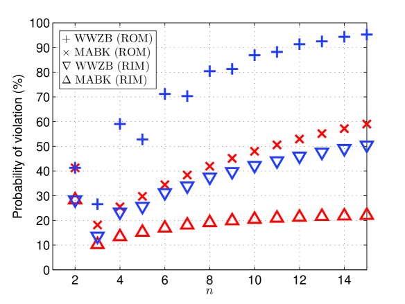
Figure 1: (Color online) Probability of finding a nonclassical $n$-partite GHZ correlation. The two sets of data at the bottom and top are, respectively, for correlation generated from random isotropic measurements (RIM) and random orthogonal measurements (ROM). The markers are for the scenarios when the verifier has access to (1) the $2^{n+1}$ MABK inequalities ($\Delta$ for RIM, $\times$ for ROM), and (2) the $2^{2^{n}}$ WWZB inequalities ($\nabla$ for RIM, $+$ for ROM).

The case of $n=2$ appears somewhat anomalous. The reason is that, for $n=2$, the equivalence class of Bell-CHSH inequalities obtained by relabeling $\mathcal{S}^{(2)}_{\mbox{\tiny MABK}}$ (or $\mathcal{S}_{\mbox{\tiny CHSH}}$) is both necessary and sufficient for determining if a given set of experimental statistics generated by performing two binary-outcome measurements per site admits a LCD A.Fine:PRL:1982 . In other words, in the space of measurement statistics generated by performing such measurements, all nonclassical correlations can be detected by this equivalence class of inequalities.

For $n>2$, there are (i) Bell inequalities with $n$-partite correlation functions that are not of the MABK form (2) and (ii) Bell inequalities involving less-than-$n$-partite correlation functions. To determine if a given correlation for $n>2$ is incompatible with any LCD, we need to test the measurement statistics against the complete set of Bell inequalities that are relevant to the particular experiment. For a small number of parties, this can be achieved efficiently using linear programming (see D.Gosal:PRA:042106 and the supplementary materials attached below) or by checking the correlation directly against the complete set of relevant Bell inequalities. Our results are summarized in Table 1.

$n$	2	3	4	5	6
RIM	28.3185%	74.6899%	94.2380%	99.5926%	$99.97\%$
$\tfrac{\text{Run}}{10^{5}}$	-	5000	500	25	0.8
ROM	41.2982%	96.2073%	99.9757%	$99.9999\%$	$100.00\%$
$\tfrac{\text{Run}}{10^{5}}$	5000	5000	500	25	0.8

Table 1: Probability of finding a nonclassical correlation from the $n$-partite GHZ state for the scenario where each party is allowed to perform binary projective measurements in two randomly chosen measurement bases. The number of data points (Run) used to compute the probabilities for RIM (ROM) is included in the third (fifth) row of the table.

These results clearly indicate that the probability of a violation rapidly approaches unity with increasing $n$. The input to the linear program, however, scales exponentially with $n$ (see supplementary materials attached below), thus making it intractable to determine the probability of violation reliably for larger values of $n$. To obtain some insight into the behavior, we can restrict our attention to the extensive set of $2^{2^{n}}$ $n$-partite correlation inequalities discovered independently by Werner & Wolf WW:Complete:npartiteBI and Żukowski & Brukner ZB:Complete:npartiteBI (WWZB). While violation of these inequalities is still sufficient to rule out LCD, the converse is generally not true. Thus, using this set of inequalities yields a lower bound on the probability that a given correlation is nonclassical.

To test if a given correlation satisfies all of the WWZB inequalities is equivalent to testing if it satisfies the following nonlinear inequality WW:Complete:npartiteBI ; ZB:Complete:npartiteBI

$$\sum_{k_{1},\ldots,k_{n}=\pm 1}\Bigl{|}\sum_{s_{1},\ldots,s_{n}=1}^{2}\prod_{j=1}^{n}k_{j}^{s_{j}-1}E(s_{1},\ldots,s_{n})\Bigr{|}\leq 2^{n}.$$ (5)

We have numerically computed the probability of finding a randomly generated correlation from RIM to violate inequality (5) for $n\leq 15$. As can be seen in Fig. 1, this probability generally increases with $n$ and is above 50% for $n=15$. However, it is inconclusive whether this probability asymptotes to unity or not for large $n$.

Finally, we consider another mechanism by which parties who do not share a reference frame can increase the probability of observing a violation. So far we have considered each of the two local measurement bases for each party to be chosen independently and isotropically. However, because the optimal violations are typically found when the pair of local measurement directions are orthogonal V.Scarani:JPA:2001 , we can consider a random selection of measurement bases under the constraint that each local pair are orthogonal. We have repeated the above calculations with this constraint (i.e., that $\Omega^{[k]}_{1}\cdot\Omega^{[k]}_{2}=0$); we refer to this distribution as random orthogonal measurements (ROM). The results reveal a significant increase in the probability of a violation, as shown in Fig. 1 and Table 1. For larger values of $n$, our results for the WWZB inequalities also strongly suggest that the probability asymptotes to unity for large $n$.

Our results so far have all made use of a fixed maximally-entangled pure state (1) (although clearly the local bases in which this state is defined are irrelevant for our result). We can also consider how the probability of observing a violation of LCD varies with the degree of entanglement of the distributed quantum state. For $n=2$, a pure quantum state can always be written as $|\Psi\rangle=\cos\theta|0\rangle_{1}|0\rangle_{2}+\sin\theta|1\rangle_{1}|1\rangle_{2}$ for some local bases. Numerically, we can compute the probability of violation as a function of entanglement (for details, see supplementary materials attached below). With this result, we can determine the probability of observing a violation of LCD using both randomly chosen measurement bases and a randomly chosen state. We sample two-qubit pure states randomly and uniformly from $\mathbb{C}^{2}\otimes\mathbb{C}^{2}$ according to the SU(4) Haar measure. Given that our results are independent of local choice of bases, we can reproduce this distribution by sampling Schmidt coefficients as for single-qubit mixed states from the uniform Bloch ball I.Bengtsson:Book . The relevant measure is the Hilbert-Schmidt measure on a single qubit, i.e., $P_{\mbox{\tiny HS}}(r)=24r^{2}$, where $r=\frac{\cos 2\theta}{2}$ is the length of the Bloch vector (pp. 354, Ref. I.Bengtsson:Book ). The probability of violation for a randomly chosen pure two-qubit state can then be determined by numerical integration to be, respectively, about 5.3% for RIM and 10.1% for ROM.

Conclusion and other directions.– We introduced the idea of performing a Bell experiment using randomly-chosen measurement bases, with the aim of demonstrating nonclassical correlations in the absence of a shared reference frame. We applied this idea to the $n$-partite GHZ state and showed that the probability of finding a nonclassical correlation rapidly tends to unity as the number of parties increases. Naively, one might have expected that this chance would diminish with increasing $n$, due to the increasing chance of misalignment of the experimenters’ measurement bases (or, alternatively, by considering the fragility of the GHZ state to dephasing). Our results clearly show otherwise. We have thus showed that without a shared reference frame, a Bell inequality violation can still be demonstrated reliably without resorting to complicated state preparation or consumption of expensive quantum resources. This, of course, significantly reduces the technical requirements for experimentally violating a Bell inequality, performing quantum key distribution based on such violations, or establishing large-scale quantum networks.

Our work also represents the first systematic study of the set of correlation derivable from a quantum resource such as the $n$-partite GHZ state. Specifically, our results indicate that the correlations obtained by performing projective measurements on this quantum resource are almost ubiquitously nonclassical (this can be rigorously quantified by considering a volume measure in the space of GHZ-attainable-correlations induced by RIM and ROM). Given that measurements and the resulting correlations play an important role in many quantum information processing tasks, the tools and ideas that we have introduced here, suitably generalized, may shed some light on the origin of the power of other quantum resources such as the highly entangled cluster state. In particular, they may add new insights to the computational power of correlations recently discussed in Ref. J.Anders:PRL:050502 .

The results presented here motivate several additional research directions. First, one may attempt to determine a new intuition for our result of increasing probability of violation with the number of parties $n$, by relating this probability to the average magnitude of the MABK violation, which also increases with $n$. Second, for many quantum information processing tasks, violation of the inequalities considered in the present work may not be sufficient, as other types of multipartite entanglement (perhaps different from that of the GHZ state) may be required that are not quantified by these inequalities. To this end, it will be interesting to investigate the efficiency of random measurements against inequalities that detect other, more general types of multipartite entanglement FullEntanglement . Finally, for real-world applications of these results, a critical issue is to determine how robust they are against decoherence.

I Supplementary Materials

I.1 MABK-violation without classical post-processing

In the main text, we have presented the probability of observing a violation by considering all equivalent Mermin-Ardehali-Belinskiǐ-Klyshko (MABK) inequalities. If the classical post-processing to optimize over the measurement labelings is not carried out (i.e., we calculate the probability to violate a particular inequality rather than an equivalent set), then we find $p^{|\mbox{\tiny GHZ}_{n}\rangle}_{\mbox{\tiny MABK}}$ decreases steadily with $n$; see Fig. 2. However, in this case, among those choices of bases that give rise to an MABK-violation, we find that their average violation increases with $n$ when normalized by the classical threshold $2^{n-\frac{1}{2}}$ but decreases when normalized by the maximal possible quantum violation $2^{\frac{3n}{2}-1}$ MerminIneq ; WW:Complete:npartiteBI . See also Ref. I.Pitowsky:PRA:022103 in this regard.

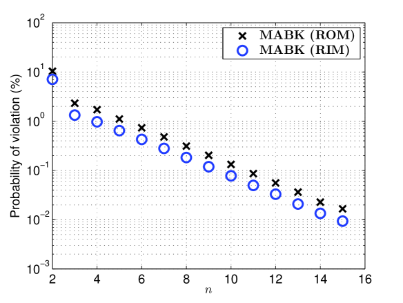
Figure 2: (Color online) Probability of finding a randomly generation correlation from $|\rm GHZ\rangle_{n}$ to violate a single MABK inequality.

I.2 Analytic derivation of probability of violation for $n=2$

For the specific case of $n=2$, the probability of violating the (2-party) MABK inequality, i.e., the Bell-CHSH inequality Bell ; CHSH

$$\mathcal{S}_{\mbox{\tiny CHSH}}=|E(1,1)+E(1,2)+E(2,1)-E(2,2)|\leq 2,$$ (6)

can be computed analytically. To this end, it is expedient to consider the two-qubit singlet state

$$|\Psi^{-}\rangle=\tfrac{1}{\sqrt{2}}\left(|0\rangle_{1}|1\rangle_{2}-|1\rangle_{1}|0\rangle_{2}\right),$$ (7)

instead of the 2-party GHZ state:

$$|{\rm GHZ}\rangle_{2}=\tfrac{1}{\sqrt{2}}\left(|0\rangle_{1}|0\rangle_{2}+|1\rangle_{1}|1\rangle_{2}\right).$$ (8)

Clearly, these states are local unitarily equivalent, and hence their probability of violating the Bell-CHSH inequality via random isotropic measurements (ROM) is identical. However, $|\Psi^{-}\rangle$ is also rotationally invariant (i.e., $U\otimes U|\Psi^{-}\rangle=|\Psi^{-}\rangle$ for arbitrary qubit unitary transformation $U$), which allows us to simplify our analysis considerably.

Let us begin by writing the measurement directions for Alice and Bob as $\vec{a}_{s_{1}}$ and $\vec{b}_{s_{2}}$. From some simple calculation, one can show that the correlation function, i.e., the average of the product of measurement outcomes for Alice measuring $\vec{a}_{s_{1}}\cdot\vec{\sigma}$ and Bob measuring $\vec{b}_{s_{s}}\cdot\vec{\sigma}$ is

$$E\left(\vec{a}_{s_{1}},\vec{b}_{s_{2}}\right)=-\vec{a}_{s_{1}}\cdot\vec{b}_{s_{2}},$$ (9)

where $\vec{\sigma}=(\sigma_{x},\sigma_{y},\sigma_{z})$ is the vector of Pauli matrices. Using this in Eq. (6), we are thus interested to know how often the inequality

$$\left|\vec{a}_{1}\cdot\vec{b}_{1}+\vec{a}_{1}\cdot\vec{b}_{2}+\vec{a}_{2}\cdot\vec{b}_{1}-\vec{a}_{2}\cdot\vec{b}_{2}\right|>2.$$ (10)

holds when the unit vectors $\vec{a}_{1}$, $\vec{a}_{2}$, $\vec{b}_{1}$ and $\vec{b}_{2}$ are chosen independently, randomly and isotropically. We can simplify this by defining the two orthogonal vectors, $\vec{r}_{\perp}=\vec{b}_{1}-\vec{b}_{2}$ and $\vec{r}=\vec{b}_{1}+\vec{b}_{2}$, in terms of which inequality (10) holds if and only if

$$\left|\vec{a}_{1}\cdot\vec{r}+\vec{a}_{2}\cdot\vec{r}_{\perp}\right|>2.$$ (11)

Note that as well as being orthogonal, the vectors $\vec{r}_{\perp}$ and $\vec{r}$ have lengths satisfying,

$$\left|\vec{r}\right|=\sqrt{2(1+\vec{b}_{1}\cdot\vec{b}_{2})}=\sqrt{2(1+x)},$$

$$\left|\vec{r}_{\perp}\right|=\sqrt{2(1-\vec{b}_{1}\cdot\vec{b}_{2})}=\sqrt{2(1-x)},$$ (12)

where $x=\vec{b}_{1}\cdot\vec{b}_{2}$.

By rewriting $\vec{r}$ in terms of its unit vector $\hat{r}$ and magnitude $|\vec{r}|$, i.e., $\vec{r}=\hat{r}|\vec{r}|=\hat{r}\sqrt{2(1+x)}$, and similarly for $\vec{r}_{\perp}$, inequality (11) becomes

$$\left|\vec{a}_{1}\cdot\hat{r}\sqrt{1+x}+\vec{a}_{2}\cdot\hat{r}_{\perp}\sqrt{1-x}\right|>\sqrt{2}.$$ (13)

Now the rotational invariance of dot products ensures that in determining the fraction of measurement directions that violate inequality (13), the actual direction of $\hat{r}$ and $\hat{r}_{\perp}$ is irrelevant. With some thought, one can see that to determine this fraction, and hence the probability of violating the Bell-CHSH inequality (6) via random isotropic measurements, it suffices to sample $x$ and the dot products $\vec{a}_{1}\cdot\hat{r}$, $\vec{a}_{2}\cdot\hat{r}_{\perp}$ uniformly from the interval $[-1,1]$. Writing $\beta=\vec{a}_{1}\cdot\hat{r}$ and $\alpha=\vec{a}_{2}\cdot\hat{r}_{\perp}$, we therefore wish to find the fraction of values of $\alpha,\beta,x\in[-1,1]$ satisfying,

$$\left|\alpha\sqrt{1-x}+\beta\sqrt{1+x}\right|>\sqrt{2}.$$ (14)

This problem has a useful geometrical interpretation. The set of all points $\alpha,\beta,x\in[-1,1]$ define a cube, $\mathfrak{C}$, which encloses a volume $2^{3}$ and has faces located at $\alpha,\beta,x=\pm{1}$. To find the fraction of Alice and Bob’s measurement directions that would violate the Bell-CHSH inequality we need to find what fraction of the volume of $\mathfrak{C}$ contains points $(\alpha,\beta,x)$ satisfying the constraint of Eq. (14).

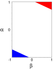
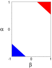
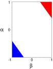
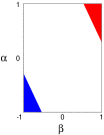
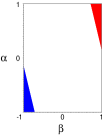
Figure 3: (Color online) Plots showing the triangular regions containing values of $\alpha$ and $\beta$ which satisfy inequality (14) (i.e., violating the Bell-CHSH inequality). From left to right, the plots are for values of $x=-0.8,-0.4,0,0.4,0.8$.

By separately considering the cases where $\alpha\sqrt{1-x}+\beta\sqrt{1+x}>0$ and $\alpha\sqrt{1-x}+\beta\sqrt{1+x}<0$, the regions of $\mathfrak{C}$ containing points satisfying Eq. (14) are given by,

$$\alpha>\frac{\sqrt{2}-\beta\sqrt{1+x}}{\sqrt{1-x}}$$ (15)

and,

$$\alpha<-\frac{\sqrt{2}+\beta\sqrt{1+x}}{\sqrt{1-x}}.$$ (16)

If we take a cross-section through $\mathfrak{C}$ corresponding to a particular fixed value of $x$, then these two expressions define triangular regions at the corners of the cube, as is shown in Fig. 3. From some straightforward computation, it can be shown that the total area of the two triangles for a given $x$ is

$$\frac{\left(\sqrt{1+x}+\sqrt{1-x}-\sqrt{2}\right)^{2}}{\sqrt{1-x^{2}}}.$$ (17)

Integrating this expression from $x=-1$ to 1, and dividing the result by $2^{3}$ (the total volume of $\mathfrak{C}$), we therefore find that the fraction of Alice and Bob’s measurement directions that will violate the Bell-CHSH inequality is:

$$\frac{\pi-3}{2}\simeq{7.0796\%}.$$ (18)

Notice that the above expression is the probability of violating inequality (6) without taking into account of any possible relabeling of measurement settings and/or outcomes. To take this into account, note that the four equivalent Bell-CHSH inequalities are as follows:

$$|E(1,1)+E(1,2)-E(2,1)-E(2,2)|\leq 2,$$ (19)

$$|E(1,1)+E(1,2)-E(2,1)+E(2,2)|\leq 2,$$ (20)

$$|E(1,1)-E(1,2)+E(2,1)+E(2,2)|\leq 2,$$ (21)

$$|-E(1,1)+E(1,2)+E(2,1)+E(2,2)|\leq 2.$$ (22)

It is not difficult to see that for any given measurement directions, at most one of these inequalities can be violated. To see this, suppose otherwise and one will find that an inequality like the following

$$E(1,1)+E(1,2)>2,$$ (23)

has to hold true. However, this is logically impossible as the absolute value of each of the correlation function $|E(s_{1},s_{2})|$ is upper bounded by 1.

Moreover, by symmetry, the probability of finding measurement directions that violate any of these equivalent inequalities is identical. Hence, the probability of finding measurement directions that violate any of the Bell-CHSH inequality, with the help of relabeling of measurement settings and/or outcomes is:

$$4\times\frac{\pi-3}{2}\simeq{28.3185\%}.$$ (24)

I.3 Identifying nonclassical correlation via linear programming

Linear programming is a convex optimization problem S.Boyd:Book:2004 which can be efficiently solved on a computer. For this kind of optimization problem, both the objective function and the constraints are linear in the variable $\mathbf{x}\in\mathbb{R}^{d}$. In its standard form, a linear program reads as S.Boyd:Book:2004 :

$$\,\text{~{}minimize}\qquad\mathbf{c}^{\mbox{\tiny T }}\mathbf{x},$$ (25a)

$$\text{~{}subject to}\quad A\mathbf{x}=\mathbf{b},$$ (25b)

$$\qquad\qquad\qquad\,\,\,\mathbf{x}\succeq\mathbf{0},$$ (25c)

where $\mathbf{c}\in\mathbb{R}^{d}$, $\mathbf{b}\in\mathbb{R}^{d^{\prime}}$, $A$ is a $d^{\prime}\times d$ matrix, $\succeq$ represents a component-wise inequality and $\mathbf{0}$ is a $d\times 1$ null vector.

For the experimental scenarios described in the main text, the $k$-th party is allowed to perform measurements in two different measurement directions $\Omega^{[k]}_{s_{k}}$, with $s_{k}=1,2$. Let us denote by $o^{[k]}_{s_{k}}$ the measurement outcome corresponding to the measurement direction $\Omega^{[k]}_{s_{k}}$. Now, recall that a given correlation admits a locally causal/ realistic description if and only if all local measurement outcomes $o^{[k]}_{s_{k}}$ are (probabilistically) determined in advance solely by the choice of the local setting $s_{k}$. Equivalently, a locally causal correlation is one where the experimental statistics admit a joint probability distribution

$$p_{1\ldots n}(o^{[1]}_{1},o^{[1]}_{2},\ldots,o^{[k]}_{1},o^{[k]}_{2},\ldots,o^{[n]}_{1},o^{[n]}_{2})$$

for all the $2n$ variables $o^{[k]}_{s_{k}}$, and which recovers all the observed experimental statistics as marginals fn:ExplicitBipartite . For example, the joint probability $p_{1n}$ of observing $o^{[1]}_{1}=1$ and $o^{[n]}_{2}=-1$, must be reproducible via:

$$p_{1n}(o^{[1]}_{1}=1,o^{[n]}_{2}=-1)$$

$$= \sum_{k=2}^{n-1}\sum_{o^{[1]}_{2},o^{[n]}_{1},o^{[k]}_{s_{k}}=\pm 1}p_{1\ldots n}(o^{[1]}_{1},o^{[1]}_{2},\ldots,o^{[k]}_{1},o^{[k]}_{2},\ldots,o^{[n]}_{1},o^{[n]}_{2});$$

likewise for all the correlation functions, such as

$$E(s_{1},s_{n})=\sum_{k=1,n}\sum_{o^{[k]}_{s_{k}}=\pm 1}\prod_{j=1,n}o^{[j]}_{s_{j}}\,p_{1n}(o^{[1]}_{s_{1}},o^{[n]}_{s_{n}}),$$

which must also be reproducible from appropriate linear combination of the entries of the joint probability distribution $p_{1\ldots n}$ (see Ref. D.Gosal:PRA:042106 for a more elaborate exposition of these constraints).

Clearly, these constraints can be put in the form of Eq. (25b), with $\mathbf{x}\in\mathbb{R}^{2^{2n}}$ being the entries of $p_{1\ldots n}$ sought for, with all (but one) entries of $\mathbf{b}\in\mathbb{R}^{3^{n}}$ being the measured correlation functions $E(s_{1},\ldots,s_{k})$, and with entries of $A$ giving the coefficients required to reproduce each $E(s_{1},\ldots,s_{k})$ from the entries of $p_{1\ldots n}$. On top of the $3^{n}-1$ correlation functions, $\mathbf{b}$ must also contain an additional entry that is set to 1; the same goes for the corresponding row of entries of $A$, which must all be set to 1. This last requirement ensures that the joint probability distribution $p_{1\ldots n}$ is normalized while the non-negativity of the probabilities is taken care of by Eq. (25c).

The problem of determining if a given correlation admits a locally causal description can then be cast as the following linear programming feasibility problem:

$$\,\text{~{}minimize}\qquad\quad\,0,$$

$$\text{~{}subject to}\quad A\mathbf{x}=\mathbf{b},$$

$$\qquad\qquad\qquad\,\,\,\mathbf{x}\succeq\mathbf{0}.$$

For an alternative formulation of the problem as a linear programming optimization problem, see Ref. M.B.Elliott:0905.2950 .

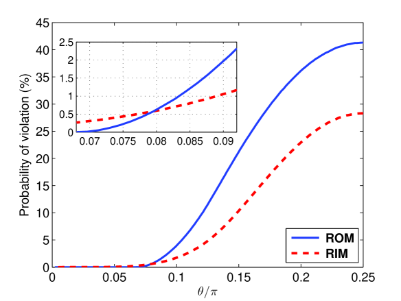
Figure 4: (Color online) Probability of finding the measurement statistics on a pure two-qubit state $|\Psi\rangle=\cos\theta|0\rangle_{1}|0\rangle_{2}+\sin\theta|1\rangle_{1}|1\rangle_{2}$ to violate the class of Bell-CHSH inequalities. Here, the largest Schmidt coefficient $\cos\theta$ quantifies the entanglement. The values $\theta=0$ and $\pi/4$ give, respectively, the pure product state and the maximally entangled two-qubit state. Inset: a magnified plot of the crossover region.

I.4 Probability of violation vs entanglement

For $n=2$, a pure quantum state can always be written as $|\Psi\rangle=\cos\theta|0\rangle_{1}|0\rangle_{2}+\sin\theta|1\rangle_{1}|1\rangle_{2}$ for some local bases. We numerically compute the probability of violation as a function of entanglement, as shown in Fig. 4. Note that, while the probability of violation is greater with ROM in most instances, it also decreases more rapidly to zero with decreasing $\theta$. In fact, at $\theta\approx 0.068\,\pi$, the probability of violation of $|\Psi\rangle$ is already close to $10^{-5}\%$ with ROM whereas the chance is still about 0.26% with RIM (inset, Fig. 4).

References

- (1) J. S. Bell, Speakable and Unspeakable in Quantum Mechanics (Cambridge University Press, Cambridge, 2004).
- (2) R. Horodecki et al., Rev. Mod. Phys. 81, 865 (2009).
- (3) J. Barrett et al., Phys. Rev. A71, 022101 (2005); N. Brunner, N. Gisin, and V. Scarani, New J. Phys. 7, 88 (2005).
- (4) A. K. Ekert, Phys. Rev. Lett. 67, 661 (1991); J. Barrett, L. Hardy, and A. Kent, ibid. 95, 010503 (2005); A. Acín, N. Gisin, and Ll. Masanes, ibid. 97, 120405 (2006); Ll. Masanes, ibid., 102, 140501 (2009).
- (5) C. H. Bennett et al., Phys. Rev. Lett. 70, 1895 (1993); R. Horodecki, M. Horodecki, and P. Horodecki, Phys. Lett. A 222, 21 (1996).
- (6) Č. Brukner et al., Phys. Rev. Lett. 92, 127901 (2004).
- (7) R. F. Werner and M. M. Wolf, Quant. Inf. Comp. 1, 1 (2001); Y.-C. Liang and A. C. Doherty, Phys. Rev. A75, 042103 (2007); Ll. Masanes, Y.-C. Liang and A. C. Doherty, Phys. Rev. Lett. 100, 090403 (2008).
- (8) J. F. Clauser et al., Phys. Rev. Lett. 23, 880 (1969).
- (9) V. Scarani and N. Gisin, J. Phys. A 34, 6043 (2001).
- (10) A. Aspect, eprint quant-ph/0402001 (2004).
- (11) S. D. Bartlett, T. Rudolph, and R. W. Spekkens, Rev. Mod. Phys. 79, 555 (2007).
- (12) S. D. Bartlett, T. Rudolph, and R. W. Spekkens, Phys. Rev. Lett. 91, 027901 (2003).
- (13) A. Cabello, Phys. Rev. A68, 042104 (2003); A. Cabello, Phys. Rev. Lett. 91, 230403 (2003).
- (14) T. Rudolph and L. Grover, Phys. Rev. Lett. 91, 217905 (2003).
- (15) F. Costa et al., New J. Phys. 11, 123007 (2009).
- (16) N. D. Mermin, Phys. Rev. Lett. 65, 1838 (1990); S. M. Roy and V. Singh, ibid. 67, 2761 (1991); M. Ardehali, Phys. Rev. A46, 5375 (1992); A. V. Belinskiǐ and D. N. Klyshko, Phys. Usp. 36 653 (1993); N. Gisin and H. Bechmann-Pasquinucci, Phys. Lett. A 246, 1 (1998).
- (17) R. F. Werner and M. M. Wolf, Phys. Rev. A64, 032112 (2001).
- (18) M. Żukowski and Č. Brukner, Phys. Rev. Lett. 88, 210401 (2002).
- (19) Ll. Masanes, Quant. Inf. Comp. 3, 345 (2003); D. Collins and N. Gisin, J. Phys. A 37, 1775 (2004).
- (20) All distinct inequalities in the MABK class can be generated by applying the different permutations ( or for all ) to the coefficients of Eq. (3) defining the inequality.
- (21) P. Lougovski and S. J. van Enk, Phys. Rev. A80, 034302 (2009).
- (22) A. Fine, Phys. Rev. Lett. 48, 291 (1982)
- (23) D. Gosal et al., Phys. Rev. A70, 042106 (2004).
- (24) I. Bengtsson and K. Życzkowski, Geometry of Quantum States: An Introduction to Quantum Entanglement (Cambridge University Press, Cambridge, 2006).
- (25) J. Anders and D. E. Browne, Phys. Rev. Lett. 102, 050502 (2009).
- (26) D. Collins et al., Phys. Rev. Lett. 88, 170405 (2002); M. Seevinck and G. Svetlichny, ibid. 89, 060401 (2002).
- (27) I. Pitowsky, Phys. Rev. A70, 022103 (2004).
- (28) S. Boyd and L. Vandenberghe, Convex Optimization (Cambridge, New York, 2004).
- (29) An explicit demonstration of this fact for the scenario was first given by Fine in Ref. A.Fine:PRL:1982 .
- (30) M. B. Elliott, e-print arXiv:0905.2950 (2009).