3D molecular line formation in dwarf carbon-enhanced metal-poor stars

Abstract

We present a detailed analysis of the carbon and nitrogen abundances of two dwarf carbon-enhanced metal-poor (CEMP) stars: SDSS J1349-0229 and SDSS J0912+0216. We also report the oxygen abundance of SDSS J1349-0229. These stars are metal-poor, with [Fe/H] $<$ –2.5, and were selected from our ongoing survey of extremely metal-poor dwarf candidates from the Sloan Digital Sky Survey (SDSS). The carbon, nitrogen and oxygen abundances rely on molecular lines which form in the outer layers of the stellar atmosphere. It is known that convection in metal-poor stars induces very low temperatures which are not predicted by ‘classical’ 1D stellar atmospheres. To obtain the correct temperature structure, one needs full 3D hydrodynamical models. Using CO5BOLD 3D hydrodynamical model atmospheres and the Linfor3D line formation code, molecular lines of CH, NH, OH and C₂ were computed, and 3D carbon, nitrogen and oxygen abundances were determined. The resulting carbon abundances were compared to abundances derived using atomic C i lines in 1D LTE and NLTE. For one star, SDSS J1349-0229, we were able to compare the 3D oxygen abundance from OH lines to O i lines in 1D LTE and NLTE. There is not a good agreement between the carbon abundances determined from C₂ bands and from the CH band, and molecular lines do not agree with the atomic C i lines. Although this may be partly due to uncertainties in the transition probabilities of the molecular bands it certainly has to do with the temperature structure of the outer layers of the adopted model atmosphere. In fact the discrepancy between C₂ and CH is in opposite directions when using 3D and 1D models. Confronted with this inconsistency, we explore the influence of the 3D model properties on the molecular abundance determination. In particular, the choice of the number of opacity bins used in the model calculations and its subsequent effects on the temperature structure and molecular line formation is discussed.

1 Introduction

SDSS J1349-0229 and SDSS J0912+0216 were selected from our ongoing survey of extremely metal-poor star candidates from the Sloan Digital Sky Survey. SDSS J1349-0229 has an effective temperature of 6200 K, log $g$ = 4.00 and [Fe/H] = –3.0. SDSS J0912+0216 is slightly hotter with a temperature of 6500 K, log $g$ = 4.50 and [Fe/H] = –2.5. These two stars belong to the class CEMP-r+s, since their atmospheres are enhanced in carbon, and show overabundances of $s$ and $r$-process elements. For details on the abundances of the neutron-capture elements, see Behara et al. (2009).

The focus of this study is on the abundances of CEMP stars determined predominately using molecular lines: carbon, nitrogen and oxygen. It is known that overcooling in the outermost layers of metal-poor stars produced by convection is not predicted by classical 1D stellar atmospheres and is best reproduced by 3D hydrodynamical simulations (Asplund et al. 1999; Caffau & Ludwig 2007; González Hernández et al. 2008). An accurate description of these outer layers is crucial for the determination of the molecular abundances.

Fortunately these two CEMP stars are hot enough to display atomic carbon lines. These lines are formed much deeper in the atmosphere compared to molecular lines, and are thus shielded from the overcooled region of the atmosphere, allowing for a validity check of the abundances obtained from molecular lines.

2 Abundance analysis

In our analysis, we used 3D model atmospheres computed with the CO⁵BOLD code (Freytag et al. 2002; Wedemeyer et al. 2004). The 3D spectral synthesis calculations were performed with the code Linfor3D. The parameters of the 3D models used are listed in Table 1.

Table 1: Parameters of the 3D models. The model $a$ was used in the analysis of SDSS J1349-0229. We interpolated between the corrections from the models $b$ for SDSS J0912+0216. The first five models were computed using 6 opacity bins, while the last three using 12 bins - see discussion for details.

Model	Teff	log $g$	[Fe/H]
d3t63g40mm30n01a	6270	4.00	–3.0
d3t65g45mm20n01b	6530	4.50	–2.0
d3t65g45mm30n01b	6550	4.50	–3.0
d3t63g40mm20n01	6280	4.00	–2.0
d3t63g40mm10n01	6260	4.00	–1.0
d3t63g40mm30n02	6240	4.00	–3.0
d3t63g40mm20n02	6250	4.00	–2.0
d3t63g40mm10n02	6250	4.00	–1.0

We compared each of our 3D models to a corresponding standard hydrostatic 1D model, and define the 3D correction of an abundance measure in the sense 3D – 1D. The 1D models are calculated using plane-parallel geometry and employ the same equation-of-state and opacities as the CO⁵BOLD models.

With the exception of C₂, all of the abundances were determined using equivalent widths of unblended lines. The C₂ abundance was determined by line fitting using the same code used by Caffau et al. (2005). For CH, we adopted the line list used by Bonifacio et al. (1998), for the UV OH lines the $gf$ values have been computed from the lifetimes calculated by Goldman & Gillis (1981), and for C₂ and NH we used the molecular line lists by Kurucz (2005). The results for the two stars are listed in Table 2.

Table 2: 3D and 1D abundances expressed with respect to solar abundances of log ($\epsilon$) = 8.50, 7.86, and 8.76 for carbon, nitrogen and oxygen, respectively.

	SDSS J1349-0229
Element	[X/Fe]1D	[X/Fe]3D
CH	2.82	2.09
C2	3.16	1.72
C i NLTE	2.42	2.51
NH	1.60	0.67
OH	1.88	1.70
O i NLTE	1.63	1.69
	SDSS J0912+0216
CH	2.17	1.67
C i NLTE	1.38	1.44
NH	1.75	1.07

3 Discussion

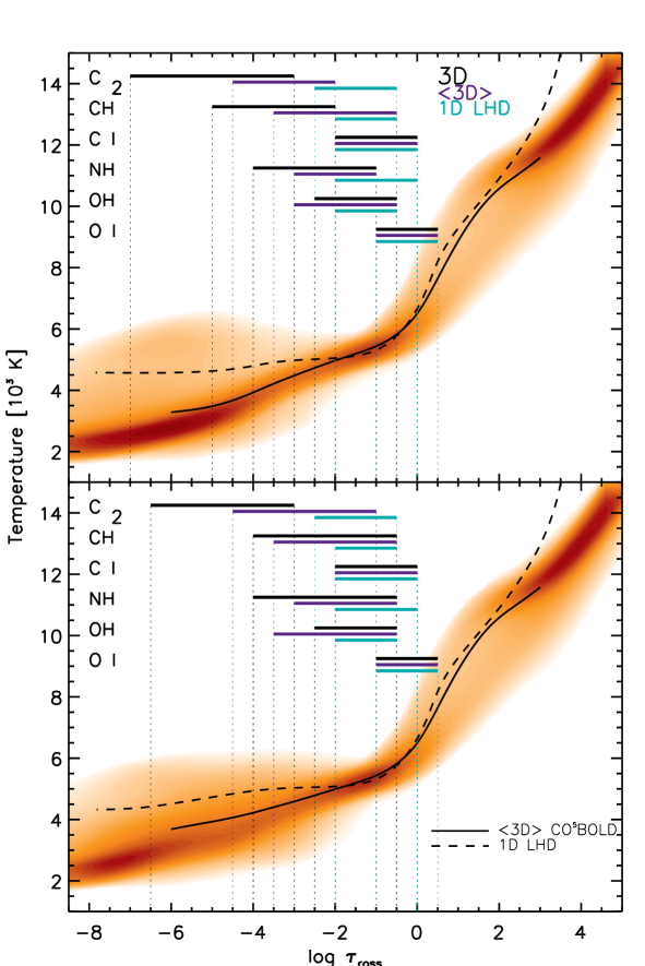
Figure 1: The temperature structures of the 3D 6 bin model d3t63g40mm30n01 (top) and 12 bin model d3t63g40mm30n02 (bottom) are plotted as a function of optical depth along with the average 3D (solid line) and corresponding 1D (dashed line) temperature structures. Overplotted on the figure are the ranges of depth of formation of the C₂, CH, C i, NH, OH and O i spectral lines used in the analysis.

The sensitivity of the molecular lines to temperature is clear from the significant 3D corrections. In Figure 1 we have plotted the temperature distributions for the models used in the analysis of SDSS J1349-0229. The ranges of depth of formation of the lines used in the analysis are overplotted for comparison. The different depth of formation of the C₂ and CH lines in the 1D and 3D models explains why in 1D we derive a larger C abundance from the C₂ lines than from the CH lines, while in 3D the reverse is true. The C₂ lines are formed much higher up in the atmosphere compared to the CH lines, and this tendency is much larger in the 3D than in the 1D model. The 3D models on the other hand do not achieve a better consistency between CH and C₂ lines. The C i lines are quite insensitive to 3D effects. Neither in 3D nor in 1D we achieve consistent results between molecular lines and C i lines.

To shed light on the discrepancy between the carbon abundance indicators, we use our best indicator, C i, as a reference and explore the influence of the 3D model properties on the molecular abundance determination. In particular, we explore the effect of increasing the number of opacity bins in the opacity groups from 6 bins to 12 bins as described in Ludwig et al. (2009). The new abundance obtained for SDSS J1349-0229 are listed in Table 3.

Table 3: Comparison between 3D abundances derived using models with 6 and 12 opacity bins.

Element	6 bin [X/Fe]3D	12 bin [X/Fe]3D
CH	2.09	2.22
C2	1.72	1.99
C i NLTE	2.51	2.50
NH	0.67	0.87
OH	1.69	1.69
O i NLTE	1.69	1.68

The temperature distribution of the 12 bin model is shown in Figure 1 below the 6 bin model. The different binning scheme results in a decrease of the overcooling, thus lowering the 3D corrections of the molecules formed higher in the atmosphere.

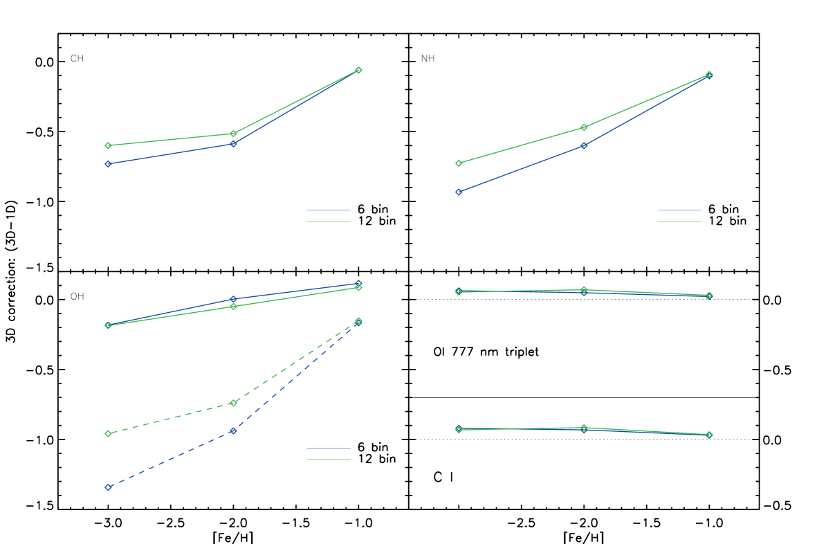
Figure 2: 3D corrections as a function of metallicity for CH, OH, NH, O i and C i. The 6 bin models are plotted in black, while the 12 bin models are plotted in grey. The OH correction have been calculated assuming a typical CEMP composition: an enhanced carbon-to-oxygen ratio of +1.0. Overplotted as dashed lines are the corrections using scaled solar abundances.

The atomic lines, formed deeper in the atmosphere are unaffected. The 12 bin models give a better agreement between the CH the C₂ lines and both molecular features appear to be in better agreement with the C i. Although these results appear encouraging, the formation region is so external and at low density, that the validity of LTE for molecule formation and levels population should be questioned.

To explore the sensitivity of the models to the different binning schemes, we compute 3D corrections for CH, C i, NH, OH and O i for [Fe/H] = –3.0, –2.0 and –1.0 using the models listed in Table 1. The corrections are shown in Figure 2. The OH lines computed using scaled-solar abundances appear the most sensitive. In carbon-enhanced atmospheres however, the effect is much reduced. Overall, with regards to the molecular lines, the sensitivity to the binning scheme as well as the 3D corrections decrease with increasing metallicity. The atomic lines proved to be immune to both the 3D model properties and 3D effects.