Higher-order brane gravity models

Abstract

We discuss a very general theory of gravity, of which Lagrangian is an arbitrary function of the curvature invariants, on the brane. In general, the formulation of the junction conditions (except for Euler characteristics such as Gauss-Bonnet term) leads to the powers of the delta function and requires regularization. We suggest the way to avoid such a problem by imposing the metric and its first derivative to be regular at the brane, the second derivative to have a kink, the third derivative of the metric to have a step function discontinuity, and no sooner as the fourth derivative of the metric to give the delta function contribution to the field equations. Alternatively, we discuss the reduction of the fourth-order gravity to the second order theory by introducing extra scalar and tensor fields: the scalaron and the tensoron. In order to obtain junction conditions we apply two methods: the application of the Gauss-Codazzi formalism and the application of the generalized Gibbons-Hawking boundary terms which are appended to the appropriate actions. In the most general case we derive junction conditions without assuming the continuity of the scalaron and the tensoron on the brane. The derived junction conditions can serve studying the cosmological implications of the higher-order brane gravity models.

1 1. Introduction

In recent years there have been growing interest both in brane universes RS ; brane1 and in the higher-order gravity theories of which the simplest is $f(R)$ gravity f(R) . In this talk we are going to combine both ideas and formulate the higher-order gravities on the brane. It emerges that the formulation is a bit non-trivial, since one faces ambiguities of the quadratic delta function contributions to the field equations. We will say how to avoid these problems and show how the Israel junction conditions for such higher-order brane gravity models can be formulated.

2 2. Fourth-order gravities.

When one considers the general gravity theories (e.g. clifton ; braneR2 ):

$$S=\chi^{-1}\int d^{D}\sqrt{-g}f(X,Y,Z)$$ (1)

in a D-dimensional spacetime ($\chi=$ const.), where $X,Y,Z$ are curvature invariants

$$X=R,\hskip 11.38092ptY=R_{ab}R^{ab},\hskip 11.38092ptZ=R_{abcd}R^{abcd},$$ (2)

then one immediately faces the 4th order field equations, except when they reduce to the theories with Euler densities of the n-th order $I^{(n)}$ lovelock

$$S=\int_{M}d^{D}x\sqrt{-g}\sum_{n}\kappa_{n}I^{(n)}~{},$$ (3)

the lowest of them being the cosmological constant $I^{(0)}=1$ ($\kappa_{0}=-2\Lambda(2\kappa^{2})^{-1}=-2\Lambda/16\pi G$), the Ricci scalar $I^{(1)}=R$ ($\kappa_{1}=(2\kappa^{2})^{-1}$), and the Gauss-Bonnet density $I^{(2)}=R{GB}=R^{2}-4R_{ab}R^{ab}+R_{abcd}R^{abcd}$ ($\kappa_{2}=\alpha(2\kappa^{2})^{-1}$, $\alpha=$ const.).

However, the theories based on the Lagrangians which are the functions of the Euler densities such as

$$f(R)=f(X),\hskip 42.67912ptf(R_{GB})=f(Z-4Y+X^{2})~{},\hskip 42.67912ptf=f(I^{(n)})$$ (4)

are again fourth-order.

3 3. Formulation of the 4th order gravities on the brane - Israel formalism.

In the context of the recent interest in string/M-theory, it is interesting to formulate the general gravity theories (1) within the framework of the brane models PRD08 . The full brane action for such a theory reads as

$$S = \chi^{-1}\int_{M}d^{D}x\sqrt{-g}f(X,Y,Z)+S_{brane}+S_{m}~{},$$ (5)

with the total energy-momentum tensor

$$T_{a}^{~{}b}=T_{a}^{~{}b~{}-}\theta(-w)+T_{a}^{~{}b~{}+}\theta(w)+\delta(w)S_{a}^{~{}b},$$ (6)

where $S_{a}^{~{}b}$ is the energy-momentum tensor on the brane, and $T_{a}^{~{}b~{}\pm}$ are the energy-momentum tensors on the both sides of the brane, $\theta(w)$ is the Heaviside step function, and $\delta(w)$ is the Dirac delta function.

We assume Gaussian normal coordinates, i.e., $(\mu,\nu=0,1,2,\ldots,D-2;w=D)$

$$ds^{2}=g_{ab}dx^{a}dx^{b}=\epsilon dw^{2}+h_{\mu\nu}dx^{\mu}dx^{\nu}~{},$$ (7)

where $\epsilon=\vec{n}\cdot\vec{n}=+1$ for a spacelike hypersurface, $\epsilon=-1$ for a timelike hypersurface, and $h_{ab}=g_{ab}-\epsilon n_{a}n_{b}$ is a projection tensor onto a $(D-1)$-dimensional hypersurface, $\vec{n}$ is the normal vector to the hypersurface. In these coordinates the extrinsic curvature is

$$K_{\mu\nu}=-{1\over 2}{\partial h_{\mu\nu}\over\partial w}~{},$$ (8)

and the Gauss-Codazzi equations read brane2

$$R_{w\mu w\nu} = {\partial K_{\mu\nu}\over\partial w}+K_{\rho\nu}K^{\rho}_{\,\,\mu},$$ (9)

$$R_{w\mu\nu\rho} = \nabla_{\nu}K_{\mu\rho}-\nabla_{\rho}K_{\mu\nu},$$ (10)

$$R_{\lambda\mu\nu\rho} = ~{}^{(D-1)}R_{\lambda\mu\nu\rho}+\epsilon\left[K_{\mu\nu}K_{\lambda\rho}-K_{\mu\rho}K_{\lambda\nu}\right]~{}.$$ (11)

In the standard Israel approach israel66 one assumes that at the brane position $w=0$:

$$h^{-}_{\mu\nu} = h^{+}_{\mu\nu}~{},$$ (12)

$$h^{-}_{\mu\nu,w} \neq h^{+}_{\mu\nu,w}~{},\hskip 14.22636ptK^{-}_{\mu\nu}\neq K^{+}_{\mu\nu}~{},$$ (13)

i.e., the metric is continuous but it has a kink, its first derivative has a step function discontinuity, and its second derivative gives the delta function contribution.

In terms of $\theta(w)$ and $\delta(w)$ functions this is equivalent to

$$h_{\mu}{{}_{\nu}}(w) = h^{-}_{\mu\nu}(w)\theta(-w)+h^{+}_{\mu\nu}(w)\theta(w)~{},$$ (14)

$${\partial h_{\mu\nu}}\over\partial w = {\partial h^{+}_{\mu\nu}\over\partial w}\theta(-w)+{\partial h^{-}_{\mu\nu}\over\partial w}\theta(w)~{},$$ (15)

$${\partial{{}^{2}}{h_{\mu}{{}_{\nu}}}\over\partial w{{}^{2}}} = {\partial{{}^{2}}h^{-}_{\mu\nu}\over\partial w{{}^{2}}}\theta(-w)+{\partial{{}^{2}}h^{+}_{\mu\nu}\over\partial w{{}^{2}}}\theta(w)$$ (16)

$$+ \left({\partial h^{-}_{\mu\nu}\over\partial w}-{\partial h^{+}_{\mu\nu}\over\partial w}\right)\delta(w)~{}.$$

For the standard brane models with the Einstein-Hilbert action in the bulk

$$S=\frac{1}{2\kappa^{2}}\int_{M}d^{D}x\sqrt{-g}R+S_{brane}+S_{m}$$ (17)

the field equations read as brane2

$$G^{w}_{~{}w} = -{1\over 2}~{}^{(D-1)}R+{1\over 2}\epsilon\left[K^{2}-Tr(K^{2})\right]=\kappa^{2}T^{w}_{~{}w},$$ (18)

$$G^{w}_{~{}\mu} = \epsilon\left[\nabla_{\mu}K-\nabla_{\nu}K^{\nu}_{\,\,\mu}\right]=\kappa^{2}T^{w}_{~{}\mu},$$ (19)

$$G^{\mu}_{~{}\nu} = ~{}^{(D-1)}G^{\mu}_{~{}\nu}+\epsilon\left[{\partial K^{\mu}_{~{}\nu}\over\partial w}-\delta^{\mu}_{~{}\nu}{\partial K\over\partial w}\right]$$

$$+ \epsilon\left[-KK^{\mu}_{~{}\nu}+{1\over 2}\delta^{\mu}_{~{}\nu}Tr(K^{2})+{1\over 2}\delta^{\mu}_{~{}\nu}K^{2}\right]=\kappa^{2}T^{\mu}_{~{}\nu}~{}.$$

and in the limit $\lim_{w\to 0}\int_{-w}^{w}$, which “fishes out” the delta function contributions, one gets the standard Israel junction conditions as brane2 :

$$\epsilon\{[K^{\mu}_{~{}\nu}]-\delta^{\mu}_{~{}\nu}[K]\} = \kappa^{2}{S}^{\mu}_{~{}\nu},\hskip 14.22636pt[K^{\mu}_{~{}\nu}]\equiv K^{\mu~{}+}_{~{}\nu}-K^{\mu~{}-}_{~{}\nu}.$$ (21)

By $[X]=X^{+}+X^{-}$ we define a jump of an appropriate quantity $X$ at the brane.

However, for the general $f(X,Y,Z)$ theory on the brane, the standard continuity relations (12)-(13) do not work. This can be seen from the field equations of the action (1)

$$P_{ab} = \frac{\chi}{2}T_{ab},$$ (22)

$$P^{ab} = -\frac{1}{2}fg^{ab}+f_{X}R^{ab}+2f_{Y}R^{c(a}{R^{b)}}_{c}+2f_{Z}R^{edc(a}{R^{b)}}_{cde}$$ (23)

$$+ f_{X;cd}(g^{ab}g^{cd}-g^{ac}g^{bd})+\square(f_{Y}R^{ab})+g^{ab}(f_{Y}R^{cd})_{;cd}$$

$$- 2(f_{Y}R^{c(a})_{;\;\;c}^{\;b)}-4(f_{Z}R^{d(ab)c})_{;cd},$$

where $f_{X}={\partial f/\partial X}$ etc.

Take, for example, the square of the Ricci scalar

$$R = ~{}^{(D-1)}R+\epsilon\left[2h^{\mu\nu}{\partial K_{\mu\nu}\over\partial w}+3Tr(K^{2})-K^{2}\right]~{},$$

where $K\equiv K^{\mu}_{\,\,\mu}$ , $Tr(K^{2})\equiv K^{\mu\nu}K_{\mu\nu}$, and appropriately, of the Ricci tensor, and of the Riemann tensor. These squares produce the terms of the type

$${\partial^{2}h^{\mu\nu}\over\partial^{2}w}{\partial K_{\mu\nu}\over\partial w},{\partial K_{\mu\nu}\over\partial w}{\partial K^{\mu\nu}\over\partial w},\left({\partial K\over\partial w}\right)^{2}~{},$$ (24)

which are proportional to $\delta^{2}(w)$, and so they are ambiguous.

Amazingly, all these ambiguous terms cancel each other exactly in the case of the Euler densities meissner01 . In fact, the junction conditions for one of the Euler densities – the Gauss-Bonnet density, were already obtained as deruelle00 ; davis

$$2\alpha\left(3[J_{\mu\nu}]-[J]h_{\mu\nu}-2[P]_{\mu\rho\nu\sigma}[K]^{\rho\sigma}\right)+[K_{\mu\nu}]-[K]h_{\mu\nu}=-\kappa^{2}S_{\mu\nu}~{},$$ (25)

where

$$P_{\mu\rho\nu\sigma} = R_{\mu\rho\nu\sigma}+2h_{\mu[\sigma}R_{\nu]\rho}+2h_{\rho[\nu}R_{\sigma]\mu}+Rh_{\mu[\nu}h_{\sigma]\rho}~{},$$ (26)

$$J_{\mu\nu} = \frac{1}{3}\left(2KK_{\mu\sigma}K^{\sigma}_{\nu}+K_{\sigma\rho}K^{\sigma\rho}K_{\mu\nu}-2K_{\mu\rho}K^{\rho\sigma}K_{\sigma\nu}-K^{2}K_{\mu\nu}\right)~{}.$$ (27)

In the limit $\alpha\to 0$, they just give Einstein-Hilbert action junction conditions (21).

In view of the ambiguities of the terms in (24), we find two ways to formulate the junction conditions for general $f(X,Y,Z)$ theories on the brane.

3.1 A. Smoothing out the continuity conditions for the metric tensor at the brane

In order to do that we impose more regularity onto the metric tensor at the brane position, i.e., we consider a singular hypersurface of the order three israel66 which fulfills the conditions (compare (12)-(13))

$$h^{-}_{\mu\nu} = h^{+}_{\mu\nu}~{},$$ (28)

$$h^{-}_{\mu\nu,w} = h^{+}_{\mu\nu,w}~{},\hskip 14.22636ptK^{-}_{\mu\nu}=K^{+}_{\mu\nu}~{},$$ (29)

$$h^{-}_{\mu\nu,ww} = h^{-}_{\mu\nu,ww}~{},\hskip 14.22636ptK^{-}_{\mu\nu,w}=K^{+}_{\mu\nu,w}~{},$$ (30)

$$h^{-}_{\mu\nu,www} \neq h^{+}_{\mu\nu,www}~{},\hskip 14.22636ptK^{-}_{\mu\nu,ww}\neq K^{+}_{\mu\nu,ww}~{},$$ (31)

i.e., the metric and its first derivative are regular, the second derivative of the metric is continuous, but possesses a kink, the third derivative of the metric has a step function discontinuity, and no sooner than the fourth derivative of the metric on the brane produces the delta function contribution.

The physical interpretation as put in terms of the second-order theory can be that there is a jump of the first derivative of the energy-momentum tensor (e.g. jump of a pressure gradient) at the brane.

In his seminal work, Israel israel66 proposed a singular hypersurface of order two, which physically corresponded to a boundary surface characterized by a jump of the energy-momentum tensor (e.g. a boundary surface separating a star from the surrounding vacuum) which was characterized by

$$h^{-}_{\mu\nu} = h^{+}_{\mu\nu}~{},$$ (32)

$$h^{-}_{\mu\nu,w} = h^{+}_{\mu\nu,w}~{},\hskip 14.22636ptK^{-}_{\mu\nu}=K^{+}_{\mu\nu}~{},$$ (33)

$$h^{-}_{\mu\nu,ww} \neq h^{-}_{\mu\nu,ww}~{},\hskip 14.22636ptK^{-}_{\mu\nu,w}=K^{+}_{\mu\nu,w}~{},$$ (34)

i.e., the metric is regular, the first derivative of the metric is continuous, but possesses a kink, the second derivative of the metric has a step function discontinuity, and the third derivative of the metric on the brane produces the delta function contribution.

The appropriate junction conditions can be obtained as follows. We rewrite the field equations (22)-(23) as

$$\sqrt{-g}C_{ab}{W^{abd}}_{;d}+\sqrt{-g}C_{ab}V^{ab}={\chi\over 2}T^{ab}C_{ab}\sqrt{-g}~{},$$ (35)

where we have introduced is an arbitrary tensor field $C_{ab}$, and

$$W^{abd} = f_{X;c}(g^{ab}g^{cd}-g^{(ac}g^{b)d})+(f_{Y}R^{ab})^{;d}$$

$$+ g^{ab}(f_{Y}R^{cd})_{;c}-2(f_{Y}R^{d(a})^{;b)}-4(f_{Z}R^{d(ab)c})_{;c}~{},$$

$$V^{ab} = -\frac{1}{2}fg^{ab}+f_{X}R^{ab}+2f_{Y}R^{c(a}{R^{b)}}_{c}$$ (37)

$$+ 2f_{Z}R^{edc(a}{R^{b)}}_{cde}~{},$$

contain third derivatives of the metric giving a step function discontinuity, so that ${W^{abd}}_{;d}$ is proportional to $\delta(w)$. Then, we integrate both sides of the formula (35) over the volume $V$ which contains the following parts (cf. Fig. 1): $G1$, $G2$ - are the left-hand-side and the right-hand-side bulk volumes which are separated by the brane, $A1=\partial G1+A0$, $A2=\partial G2-A0$ are the boundaries of these volumes, and $A0$ is the brane which orientation is given by the direction of the normal vector $\vec{n}$.

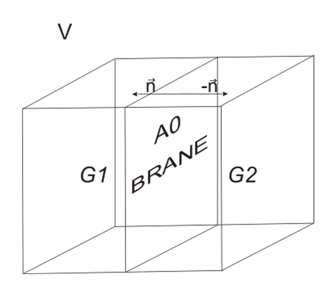
Figure 1: A schematic picture illustrating the domains of integration used in derivation of the junction conditions. Here $V=G1+G2$ is the total volume, $G1$, $G2$ - are the left-hand-side and the right-hand-side bulk volumes which are separated by the brane, $A1=\partial G1+A0$, $A2=\partial G2-A0$ are the boundaries of these volumes, and $A0$ is the brane which orientation is given by the direction of the normal vector $\vec{n}$.

We have

$$\int_{G1+G2}{\sqrt{-g}C_{ab}{W^{abd}}_{;d}d\Omega}+\int_{G1+G2}{\sqrt{-g}C_{ab}V^{ab}d\Omega}=\int_{G1+G2}{{\chi\over 2}T^{ab}C_{ab}\sqrt{-g}d\Omega}~{},$$ (38)

and so

$$\int_{G1+G2}\sqrt{-g}(C_{ab}W^{abd})_{;d}d\Omega-\int_{G1+G2}\sqrt{-g}C_{ab;d}W^{abd}d\Omega+\int_{G1+G2}\sqrt{-g}C_{ab}V^{ab}d\Omega$$ (39)

$$= \int_{G1}{\chi\over 2}T^{ab}C_{ab}\sqrt{-g}d\Omega+\int_{G2}{\chi\over 2}T^{ab}C_{ab}\sqrt{-g}d\Omega+\int_{A0}{\chi\over 2}S^{ab}C_{ab}\sqrt{-\gamma}d\sigma~{},$$

of which the first term can be integrated out to a boundary A1+A2 and then the limit $V\to A0$ (or $\lim_{w\to 0}\int_{-w}^{w}$ in Gaussian coordinates) is taken.

The final form of the junction conditions which generalize (21) onto the fourth-order gravity are

$$[W]^{abd}n_{d}-{\chi\over 2}S^{ab} = 0~{},\hskip 8.5359pt[W]^{abd}=W^{abd+}-W^{abd-}.$$ (40)

It is remarkable that these junction conditions involve the higher derivatives of the scale factor. To see this take for example $f(X,Y,Z)=f(R)$ theory in $D=5$ dimensions with metric

$$ds^{2}=-dt^{2}+a^{2}(t,w)[dr^{2}+r^{2}(d\Theta^{2}+sin^{2}\Theta d\phi^{2})]+dw^{2}~{}~{}.$$

The junction conditions (40) give a jump of the third derivative of $a(t,w)$, as expected

$$[a^{\prime\prime\prime}] = {\chi\over 2}{a_{0}}{p_{0}}~{},$$ (41)

$$p_{0} = \rho_{0}~{},$$ (42)

where $(\ldots)^{\prime}=\partial/\partial w$, $a_{0}=a(w=0)$, and the brane energy-momentum tensor is $S_{\mu}^{\nu}=(-\rho_{0},p_{0},p_{0},p_{0})$.

3.2 B. Reduction to an equivalent 2nd order theory

Yet another way to obtain the junction conditions is the reduction of the action (1) to a second-order action. This gives equivalent junction conditions, though at the expense of introducing a new tensor field $H^{abcd}$ (tensoron). In fact, starting from the action kijowski

$$S_{G} = \chi^{-1}\int_{M}d^{D}x\sqrt{-g}f(g_{ab},R_{abcd}).$$ (43)

we may transform to an equivalent 2nd order action in the form

$$S_{I}=\chi^{-1}\int_{M}d^{D}x\sqrt{-g}\{H^{ghij}(R_{ghij}-\phi_{ghij})+f(g_{ab},\phi_{cdef})\}~{},$$ (44)

where

$$H^{ghij}\equiv{\partial f(g_{ab},\phi_{abcd})\over\partial\phi_{ghij}}~{},\hskip 28.45274ptdet\left[{\partial^{2}f(g_{ab},\phi_{abcd})\over\partial\phi_{ghij}\partial\phi_{klmn}}\right]\neq 0.$$ (45)

This transition for $f(R)$ theory requires a new scalar $H=f^{\prime}(Q)$ (a scalaron) with the condition that $f^{\prime\prime}(Q)\neq 0$, and the equation of motion $Q=R$. Similarly, for $f(R_{GB})$ theory, one defines a scalar $H=f^{\prime}(A)$, with the equation of motion $A=R_{GB}$). In order to get junction conditions, we have to slightly redefine the tensoron

$$A^{abcd}={1\over 2}\{H^{acdb} + H^{abdc}-H^{cbda}-H^{acbd}-H^{abcd}+H^{cbad}\}$$ (46)

which in a particular case of $f(X,Y,Z)$ theory takes the form

$$A^{abcd}=f_{X}(g^{ad}g^{cb}-g^{cd}g^{ba})+f_{Y}(2R^{ad}g^{bc}-R^{cd}g^{ba}-R^{ba}g^{cd})+4f_{Z}R^{acbd}~{}.$$ (47)

The field equations for an equivalent action (43) read as

$$R_{ghij} = -{\partial V(g_{ab},H^{cdef})\over\partial H^{ghij}}~{},$$ (48)

$${1\over 2}g^{ab}f + {\partial f\over\partial g_{ab}}+H^{becd}\phi^{a}_{~{}ecd}(g_{ab},H^{klmn})+\{A^{(ab)cd}\}_{;dc}=-{\chi\over 2}T^{ab}~{},$$ (49)

where

$$V(g_{ab},H^{cdef})=-H^{hgij}\phi_{ghij}(g_{ab},H^{cdef})+f(g_{ab},\phi_{klmn}(g_{ab},H^{cdef}))$$ (50)

In fact, the possibility to express the fields $\phi_{abcd}$ as a function of $g_{ab}$ and $H^{cdef}$ is guaranteed by the condition (45) (which is an analogue of the condition $f^{\prime\prime}(Q)\neq 0$).

One can show that junction conditions of the second-order theory are equivalent to junction conditions of the fourth-order theory PRD08 .

Applying the same method as in the previous case (i.e. taking the limit of $V\to A0$) we notice that the first three terms of (49) do not give any contribution to the junction conditions (since they do not contain delta functions at all) which now have the form:

$$[{A^{(ab)cd}}_{;d}]n_{c}=-{\chi\over 2}S^{ab}~{}.$$ (51)

Assuming that

$$f(g_{ab},\phi_{abcd})=f({\phi_{ab}}^{ab},{\phi_{acb}}^{c}{\phi^{acb}}_{c},\phi_{abcd}\phi^{abcd}),$$ (52)

we can get the same result as in the 4th theory

$${[A^{(ab)cd}}_{;d}]n_{c} = {[A^{(ab)cd}}_{;c}]n_{d}=[-\{f_{X;c}(g^{ab}g^{cd}-g^{c(a}g^{b)d})$$ (53)

$$+ (f_{Y}R^{ab})^{;d}+g^{ab}(f_{Y}R^{cd})_{;c}$$

$$-2(f_{Y}R^{d(a})^{;b)} - 4(f_{Z}R^{d(ab)c})_{;c}\}]n_{d}=-[W^{abd}]n_{d}.$$

Similar approach was used for less-general $f(R)$ theories of gravity on the brane by Borzeszkowski and Frolov borzeszkowski ; Parry at al. branef(R) , Deruelle et al. deruelle07 , and for $f(X,Y,Z)=aX^{2}+bY+cZ$ ($a,b,c=$ const.) theories by Nojiri and Odintsov braneR2 .

4 4. Formulation of the 4th order gravities on the brane - Gibbons-Hawking Boundary Terms

In this approach, following the idea of Gibbons and Hawking GH , we do not assume any vanishing of the first derivative of the variation of the metric tensor $\delta g_{ab;c}$ on the boundary of the integration volume while using the variational principle. Strictly speaking, only the assumption of the vanishing of the normal derivative of the variation of the metric tensor $\delta g_{ab,w}$ is required. Instead, we postulate that some extra terms to the action are added and that these terms “kill” the first derivatives of the metric variation. These terms are called Gibbons-Hawking boundary terms now. In fact, the Gibbons-Hawking boundary term for the Einstein-Hilbert action is composed of the trace of the extrinsic curvature and it was found by Gibbons and Hawking themselves GH . Then, for the action being the combination of the square of the Weyl tensor and an arbitrary function of the scalar curvature they were found by Hawking and Lutrell lutrell and Barrow and Madsen madsen . For the Gauss-Bonnet and other Lovelock densities they were found by Bunch bunch81 , Mueller-Hoissen and Myers surface , Davis davis and Gravanis and Willinson gravanis . The boundary terms for the action being an arbitrary function of the curvature invariants were found by Barvinsky and Solodukhin barvinsky .

For the theories which are of interest for this talk, the Gibbons-Hawking boundary terms have the following form JCAP09 : for the $f(R)$ theory the term reads as

$$S_{GH,p}=-2(-1)^{p}\epsilon\int_{\partial M_{p}}\sqrt{-h}HKd^{D-1}x~{},$$ (54)

where $H=f^{\prime}(Q)$ is the scalaron, while for the $f(X,Y,Z)$ theory it reads as

$$S_{GH,p}=-(-1)^{p}\int_{\partial M_{p}}d^{D-1}x\sqrt{-h}A^{(ab)cd}n_{c}n_{d}\mathcal{L}_{\vec{n}}g_{ab}~{},$$ (55)

where $A^{(ab)cd}$ is the tensoron.

Using the method of the boundary terms we derived the most general Israel junction conditions for $f(R)$ theory as JCAP09 :

$$[K] = 0~{},$$ (56)

$$S^{ab}n_{a}n_{b} = 0~{},$$ (57)

$$S^{ab}h_{ac}n_{b} = 0~{},$$ (58)

$$-(D-1)[H_{;c}n^{c}]-D[H]K = \epsilon{\chi\over 2}S^{ab}h_{ab}~{},$$ (59)

$$-h_{ab}[H_{;c}n^{c}]-[H]Kh_{ab} + [HK_{ab}]$$

$$= \epsilon{\chi\over 2}S^{cd}h_{ca}h_{db}.$$

A generality of these conditions refers to the fact that no assumption about the continuity of the scalaron on the brane has been made. They reduce to the conditions already obtained in the literature, if one assumes $[H]=0$ deruelle07 .

On the other hand, the most general Israel junction conditions for the $f(X,Y,Z)$ theory, with no assumption about the continuity of the tensoron on the brane, are JCAP09 :

$$[KA^{(ab)cd}]n_{c}n_{d}+[\mathcal{L}_{\vec{n}}A^{(ab)cd}]n_{c}n_{d}$$ (62)

$$- \epsilon[A^{(ab)cd}K_{cd}]-g^{ab}[A^{(ef)cd}K_{ef}]n_{c}n_{d}$$

$$+ 2\epsilon[D_{s}A^{(ef)cd}n_{c}n_{d}]h^{s}_{e}h^{(a}_{f}n^{b)}-2\epsilon[{A^{(ab)cd}}_{;(c}]n_{d)}={\chi\over 2}S^{ab}~{},$$

$$n_{b}n_{c}[\mathcal{L}_{\vec{n}}g_{ad}]-n_{a}n_{c}[\mathcal{L}_{\vec{n}}g_{db}]-n_{b}n_{d}[\mathcal{L}_{\vec{n}}g_{ac}]+n_{a}n_{d}[\mathcal{L}_{\vec{n}}g_{cb}]=0~{}.$$

They reduce to the conditions (51), if one assumes continuity of the tensoron on the brane

$$[A^{(ab)cd}]=0~{}.$$ (63)

5 5. Fourth-order gravities and statefinders

We claim the fact that general $f(R,R_{ab}R^{ab},R_{abcd}R^{abcd})$ theories are fourth-order may have some advantageous consequences onto their observational verification by the application of statefinder diagnosis of the universe.

In fact, statefinders are the higher-order characteristics of the universe expansion which go beyond the Hubble parameter $H$ and the deceleration parameter $q$:

$$H = \frac{\dot{a}}{a}~{},\hskip 14.22636ptq=-\frac{1}{H^{2}}\frac{\ddot{a}}{a}=-\frac{\ddot{a}a}{\dot{a}^{2}}~{}.$$ (64)

They can generally be expressed as ($i\geq 2$)

$$x^{(i)} = (-1)^{i+1}\frac{1}{H^{i}}\frac{a^{(i)}}{a}=(-1)^{i+1}\frac{a^{(i)}a^{i-1}}{\dot{a}^{i}}~{},$$ (65)

and the lowest order of them are known as: jerk, snap (”kerk”), crack (”lerk”)

$$j = \frac{1}{H^{3}}\frac{\dot{\ddot{a}}}{a}=\frac{\dot{\ddot{a}}a^{2}}{\dot{a}^{3}}~{},\hskip 14.22636ptk=-\frac{1}{H^{4}}\frac{\ddot{\ddot{a}}}{a}=-\frac{\ddot{\ddot{a}}a^{3}}{\dot{a}^{4}}~{},l=\frac{1}{H^{5}}\frac{a^{(5)}}{a}=\frac{a^{(5)}a^{4}}{\dot{a}^{5}}~{},$$ (66)

and pop (”merk”), ”nerk”, ”oerk”, ”perk” etc. statefind .

In the case of the 4th order gravities, statefinders may become powerful tools to constrain such theories observationally, since they enter observational relations in the higher orders of redshift $z$ (see statefR for non-brane case diagnosis).

Apparently, a blow-up of statefinders may also be linked to an emergence of exotic singularities in the universe blowup .

6 6. Conclusions

We conclude the following:

• The formulation of the fourth-order gravity theories on the brane is non-trivial because of the powers of delta function ambiguities.

• Two methods were applied:
  A. Smoothing out the continuity conditions for the metric tensor at the brane;
  B. Reduction to an equivalent 2nd order theory.
  In both cases the Israel junction conditions have been obtained and they are also mutually equivalent.

• The method of the GH boundary terms was also applied and the most general junction conditions (with no continuity of the scalaron and tensoron on the brane assumed) were obtained that way, too.

• Higher-order brane gravities contain higher-order derivatives of the geometric quantities (in a Friedmann model it is just the scale factor) which may manifest themselves in the higher-order characteristics of expansion such as statefinders (jerk, snap, lerk/crack, merk/pop).

• A blow-up of statefinders may be linked to an emergence of exotic singularities in the universe.

References

• (1) L. Randall and R. Sundrum, Phys. Rev. Lett., 83, 3370 (1999); L. Randall and R. Sundrum, ibidem, 83, 4690 (1999).
• (2) M. Visser, Phys. Lett. B159, 22 (1985); N. Arkani-Hamed, S. Dimopoulos, and G. Dvali, Phys. Lett. B 516, 70 (1998); I. Antoniadis, N. Arkani-Hamed, S. Dimopoulos, G. Dvali, Phys. Lett. B 436, 257 (1998); N. Arkani-Hamed, S. Dimopoulos, and G. Dvali, Phys. Rev. D 59, 086004 (1999).
• (3) A.A. Starobinsky, Phys. Lett. B 91, 99 (1980); G. Magnano and L.M. SokoΕ‚owski, Phys. Rev. D 50, 5039 (1994); T.P. Sotiriou, Class. Quantum Grav. 23, 5117 (2006); G.J. Olmo, Phys. Rev. Lett. 98, 061101 (2007); G.J. Olmo, Phys. Rev. D 75, 023511 (2007); S. Capozziello, V.F. Cardone, and A. Troisi, Phys. Rev. D 71, 043503 (2005); S. Capozziello, S. Nojiri, S.D. Odintsov, and A. Troisi, Phys. Lett. B 639, 135 (2006); T. Chiba, T. Kobayashi, M. Yamaguchi, and J. Yokoyama, Phys. Rev. D 75, 043516 (2007); S. Capozziello and R. Garatini, Class. Quantum Grav. 24, 1627 (2007); L. Amendola, D. Polarski, and S. Tsujikawa, Phys. Rev. Lett. 98, 131302 (2007).
• (4) T. Clifton and J.D. Barrow, Phys. Rev. D72, 123003 (2005); Class. Quantum Grav. 23, 2951 (2006).
• (5) S. Nojiri and S.D. Odintsov, JHEP 007, 049 (2000); S. Nojiri, S.D. Odintsov and S. Ogushi, Phys. Rev. D65, 023521 (2001).
• (6) D. Lovelock, J. Math. Phys. 12, 498 (1971).
• (7) A. Balcerzak and M.P. DaΜ§browski, Phys. Rev. D77, 023524 (2008).
• (8) M. Sasaki, T. Shiromizu and K.I. Maeda, Phys. Rev. D62, 024008 (2000); T. Shiromizu, K.I. Maeda, and M. Sasaki, Phys. Rev. D62, 024012 (2000); S. Mukohyama, T. Shiromizu, and K.I. Maeda, Phys. Rev. D62, 024028 (2000).
• (9) W. Israel, Nuovo Cimento B44, 1 (1966).
• (10) K.A. Meissner and M. Olechowski, Phys. Rev. Lett. 86, 3708 (2001).
• (11) N. Deruelle and T. DoleΕΎel, Phys. Rev. D62, 103502 (2000).
• (12) A. Jakubiec and J. Kijowski, Phys. Rev. D37, 1406 (1988).
• (13) H.H. v. Borzeszkowski and V.P. Frolov, Ann. Phys. (Leipzig) 7, 285 (1980).
• (14) M. Parry, S. Pichler, and D. Deeg, JCAP 0504, 014 (2005).
• (15) N. Deruelle, M. Sasaki, and Y. Sendouda, Prog.Theor.Phys., 119, 237 (2008).
• (16) G.W. Gibbons and S.W. Hawking, Phys. Rev. D15, 2752 (1977).
• (17) S.W. Hawking and J.C. Lutrell, Nucl. Phys. B247, 250 (1984).
• (18) M. Madsen and J.D. Barrow, Nucl. Phys. B323, 242 (1989).
• (19) T.S. Bunch, Journ. Phys. A14, L139 (1981).
• (20) F. MΓΌller-Hoissen, Phys. Lett. B163, 106 (1985); R.C. Myers, Phys. Rev. D36, 392 (1987).
• (21) S.C. Davis, Phys. Rev. D67, 024030 (2003).
• (22) E. Gravanis and S. Willinson, Journ. Math. Phys. 47, 2503 (2006); Phys. Rev. D75, 084025 (2007).
• (23) A.D. Barvinsky and S.N. Solodukhin, Nucl. Phys. B479, 305 (1996).
• (24) A. Balcerzak and M.P. DaΜ§browski, JCAP 01, 018 (2009).
• (25) V. Sahni, T.D. Saini, A.A. Starobinsky, and U. Alam, JETP Lett. 77, 201 (2003); M. Visser, Class. Quantum Grav. 21, 2603 (2004); R.R. Caldwell and M. Kamionkowski, JCAP 0409, 009 (2004); M.P. DaΜ§browski and T. Stachowiak, Ann. Phys. (New York) 321, 771 (2006); M. Dunajski and G.W. Gibbons, Class. Quantum Grav. 25, 235012 (2008).
• (26) M.P. DaΜ§browski, Phys. Lett. 625, 184 (2005); M.P. DaΜ§browski, Ann. Phys. (Berlin) 15, 352 (2006).
• (27) N.J. Poplawski, Phys. Lett. B640, 135 (2006); Class. Quantum. Grav. 24, 3013 (2007); S. Capozziello, V.F. Cardone, and V. Salzano, Phys. Rev. D78, 063504 (2008).