Stellar Masses of Lyman Break Galaxies, Ly$\alpha$ Emitters and Radio Galaxies in Overdense Regions at $z=4-6$

Abstract

We present new information on galaxies in the vicinity of luminous radio galaxies and quasars at $z\simeq$4, 5, and 6. These fields were previously found to contain overdensities of Lyman Break Galaxies (LBGs) or spectroscopic Ly$\alpha$ emitters, which were interpreted as evidence for clusters-in-formation (“protoclusters”). We use HST and Spitzer data to infer stellar masses from stellar synthesis models calibrated against the Millennium Run simulations, and contrast our results with large samples of LBGs in more average environments as probed by the Great Observatories Origins Deep Survey (GOODS). The following results were obtained. First, LBGs in both overdense regions and in the field at $z=4-5$ lie on a very similar sequence in a $z^{\prime}$–[3.6] versus 3.6$\mu$m color-magnitude diagram. This is interpreted as a sequence in stellar mass ($M_{*}\sim 10^{9}$–$10^{11}$ $M_{\odot}$) in which galaxies become increasingly red due to dust and age as their star formation rate (SFR) increases, while their specific SFR stays constant. Second, the two radio galaxies are among the most massive objects ($M_{*}\sim 10^{11}$ $M_{\odot}$) known to exist at $z\simeq 4-5$, and are extremely rare based on the low number density of such objects as estimated from the $\sim$25$\times$ larger area GOODS survey. We suggest that the presence of the massive (radio) galaxies and associated supermassive black holes has been boosted through rapid accretion of gas or merging inside overdense regions. Third, the total stellar mass found in the $z=4$ protocluster TN1338 accounts for $<$30% of the stellar mass on the cluster red sequence expected to have formed at $z\gtrsim 4$, based on a comparison with the massive X-ray cluster Cl1252 at $z=1.2$. Although future near-infrared observations should determine whether any massive galaxies are currently being missed by our UV/Ly$\alpha$ selections, one possible explanation for this mass difference is that TN1338 evolves into a smaller cluster than Cl1252. This raises the interesting question of whether the most massive protocluster regions at $z>4$ remain yet to be discovered.

1. INTRODUCTION

Galaxy clusters formed in high-density regions of dark matter that collapsed earlier than surrounding low-density regions (Kaiser, 1984; Springel et al., 2005), and models predict that the galaxies that formed inside these high-density regions also may have formed earlier or evolved at an increased rate compared to their surroundings (Kauffmann, 1995; Benson et al., 2001; Thomas et al., 2005; De Lucia et al., 2006). The mass functions of clusters at low and high redshift can significantly improve current estimates of the cosmological parameters (Vikhlinin et al., 2009). Clusters of galaxies are thus important not only for the formation of dark matter structure, but also for studying processes related to galaxy formation, such as the history of gas accretion and depletion, the feedback of supernovae and active galactic nuclei (AGN), the enrichment of the intracluster medium, and the spectra-morphological transitions of galaxies.

In the local Universe, the galaxies in the centers of clusters inhibit a distinct location in the color-magnitude diagram (CMD). This cluster “red sequence” consists of predominantly spheroidal and lenticular galaxies having old stellar populations and high stellar masses, and usually includes the brightest cluster galaxy. In order to understand how and when this relation formed, it is important to study clusters at high redshifts. Traditional surveys have uncovered clusters at redshifts as high as $z\sim 1.5$ either by searching for galaxies on the characteristic red sequence or by searching for hot cluster gas in the X-rays. A red sequence of morphological early-type galaxies is prominently present in even the most distant clusters, and the small scatter in galaxy colors around the sequence has been used to infer formation redshifts of $\sim 2-5$ (e.g. Ellis et al., 1997; van Dokkum et al., 2000; Stanford et al., 2002, 2005; Blakeslee et al., 2003a, 2006; Holden et al., 2005; Postman et al., 2005; Mullis et al., 2005; Mei et al., 2006; Rettura et al., 2008).

The epoch corresponding to the assembly of massive cluster galaxies is presumed to be marked by a violent stellar mass build-up. In order to target this epoch, various techniques have been used. One technique is based on the hypothesis that at very early times the most massive galaxies trace the highest density regions and can thus be used as “lighthouses” to pinpoint possible “protoclusters”. Radio galaxies (RGs) are among the largest and most massive galaxies at $z=2-5$ ($M_{*}\sim 10^{10-12}$ M_⊙, e.g. Pentericci et al., 1997; Rocca-Volmerange et al., 2004; Seymour et al., 2007; Hatch et al., 2009, this paper), while the most luminous high redshift quasars (QSOs) have some of the largest black hole masses inferred ($M_{BH}\sim 10^{8-10}$ M_⊙, e.g. Jiang et al., 2007; Kurk et al., 2007). Overdensities (of the order of a few) of star-forming galaxies suggest that at least some radio galaxies are associated with rare peaks in the large-scale structure (e.g. Pentericci et al., 2000; Miley et al., 2004; Venemans et al., 2002, 2007). Similarly, the number counts of faint $i$-dropouts towards two $z\sim 6$ QSOs (Stiavelli et al., 2005; Zheng et al., 2006; Kim et al., 2009) also indicate a possible enhancement (see Overzier et al., 2009, for a detailed discussion). Similar overdensities have also been found in “random” fields at $z\simeq 2-6$ (e.g. Steidel et al., 1998, 2005; Shimasaku et al., 2003; Ouchi et al., 2005; Ota et al., 2008), and are consistent with being progenitors of present-day clusters.

Steidel et al. (2005) found an increase in the stellar masses and ages for star-forming galaxies in a protocluster at $z=2.3$ compared to the surrounding field. In Zirm et al. (2008) we presented evidence for a population of relatively evolved galaxies near a radio galaxy at $z=2.2$ (see also Kodama et al., 2007), and Kurk et al. (2004) found evidence for different spatial distributions of blue and red galaxies. Although Venemans et al. (2007) found no differences in the physical properties of LAEs in protoclusters compared to the field, protoclusters tend to have an elevated AGN fraction (e.g. Pentericci et al., 2002; Venemans et al., 2007; Lehmer et al., 2008). Lehmer et al. (2008) found an enhancement in the stellar masses of LBGs in the protocluster SSA22 at $z=3.1$ (Steidel et al., 1998), while Peter et al. (2007) and Overzier et al. (2008) did not find any morphological differences between UV-selected galaxies in protoclusters compared to the field using data from the Advanced Camera for Surveys (ACS) on-board the Hubble Space Telescope (HST).

The ACS, in particular, has enabled the selection of large samples of faint UV “dropout” galaxies at $z>4$ (Giavalisco et al., 2004; Bouwens et al., 2004, 2007). Combined with the great sensitivity in the mid-infrared provided by the Infrared Array Camera (IRAC) on the Spitzer Space Telescope (SST), we can study the stellar populations of those galaxies (Yan et al., 2005; Labbé et al., 2006; Eyles et al., 2007; Stark et al., 2007, 2009; Verma et al., 2007; Yabe et al., 2008). While observations in the UV probe the (dust attenuated) light from young, massive stars, the rest-frame optical light offers a more direct probe of the total stellar mass. Results at $z\sim 2-3$ imply that some LBGs and near-infrared selected galaxies were already quite massive at $z\gtrsim 5$ implying rapid evolution (e.g. Shapley et al., 2001; Papovich et al., 2001; Yan et al., 2005; Papovich et al., 2006; Wuyts et al., 2007). Recently, Stark et al. (2009) found that the $z>4$ UV luminosity function (LF) is dominated by episodic star formation ($\leq$500 Myr on average) from systems that reached their high UV luminosities in short times ($<$300 Myr), consistent with the decline in the UV LF (Bouwens et al., 2007). Galaxies having relatively high equivalent widths of Ly$\alpha$ emission (the so-called “Ly$\alpha$-emitters”) have received attention (partly due to the relative ease of their detections out to the highest redshifts) concerning the question whether they mark a particular phase in the evolution of typical starbursts (e.g. Shapley et al., 2003; Gawiser et al., 2006; Pentericci et al., 2007, 2009; Ouchi et al., 2008).

In this paper we will derive stellar masses, as inferred from the rest-frame optical fluxes, for a sample of LBGs, LAEs and RGs in two protoclusters: “TN1338” at $z\simeq 4.1$ (Venemans et al., 2002; Miley et al., 2004; Zirm et al., 2005; Overzier et al., 2008), and “TN0924” at $z\simeq 5.2$ (Venemans et al., 2004; Overzier et al., 2006). For completeness, we also present a small sample of $i$-dropouts near two quasars at $z\sim 6$ studied by Stiavelli et al. (2005) and Zheng et al. (2006). The target fields are listed in Table 1. Comparison with large samples from the GOODS survey (Giavalisco et al., 2004) will enable us to compare the overdense regions with more average environments. While the data presented here cannot compete in terms of either depth or area with other studies in the literature (e.g. Stark et al., 2009), our data is unique in the sense that we cover a few sightlines towards rare, overdense regions and luminous AGN. Specifically, we will address the following questions:
(1) How do the stellar masses of radio galaxies, LBGs and LAEs compare?
(2) Do galaxies in overdense regions at high redshift have distinct physical properties?
(3) Is the total amount of stellar mass detected in protoclusters consistent with the stellar mass in galaxies on the low redshift cluster red sequence?
(4) Have we missed a population of obscured or quiescent galaxies not selected by our UV/Ly$\alpha$ selections?

The structure of this paper is as follows: The samples and our measurement techniques are described in §2. In §3 we present the rest-frame UV-optical color-magnitude diagrams at $z\simeq 4,5,6$ and estimate stellar mass distributions based on simple model comparisons. We discuss our results in §4. All magnitudes are in the AB system. For comparison with other studies, it is convenient to specify that the characteristic luminosity $L_{z=3}^{*}$ at $z\sim 3$ (Steidel et al., 1999, i.e., $M_{1700,AB}=-21.07$) corresponds to $z$-band magnitudes of $\sim$24.9, 25.3 and 25.6 at $z$$\sim$4, 5 and 6, respectively. We adopt the following cosmological parameters: $\Omega_{M}=0.27$, $\Omega_{\Lambda}=0.73$, and $H_{0}=73$ km s^-1 Mpc^-1.

2. SAMPLES, DATA AND MEASUREMENTS

2.1. Primary Samples

2.1.1 Radio galaxy fields

This paper is based on various samples of galaxies in overdense regions selected as part of previous works (see §1). For the two radio galaxy fields we make use of large samples of LBGs and LAEs selected from our previous HST/ACS imaging and Ly$\alpha$ surveys.

In the field TN1338 we will focus on a sample of LAEs and LBGs selected near the radio galaxy TN J1338–1942 at $z=4.11$. The field covered with both HST and Spitzer contains 12 Ly$\alpha$ emitters from Venemans et al. (2007): these LAEs are part of a larger structure that is $\approx 5\pm 1$ times more dense compared to average expectations, and has a velocity dispersion of $\approx 300$ km s^-1 centered on the radio galaxy. The LBG sample consists of 66 $g_{475}$-band ($g$) dropouts brighter than $z_{850}$$=$27.0 mag. As detailed in Overzier et al. (2008), the photometric redshift distribution peaks at $z=4.1$, and has a width of $\Delta z\sim 0.5$ (FWHM). About half of the LAEs ($|z-\Delta z|<0.03$) are also selected as part of the dropout sample, indicating that the true width of the redshift distribution of the dropouts could be narrower than suggested by the photo-$z$ analysis given its fairly limited accuracy. Unfortunately, the redshifts of most of the dropouts are difficult to determine spectroscopically due to their faintness and because all high equivalent width Ly$\alpha$ sources have already been identified. Statistical studies indicate that the ratio of Ly$\alpha$-faint to Ly$\alpha$-bright LBGs in a UV flux-limited sample is about 3:1 (e.g. Shapley et al., 2003). The population of $g$-dropouts represents an overdensity at the $>5\sigma$ significance with respect to the average field as estimated from the GOODS survey, consistent with a substantial fraction lying near the redshift of the radio galaxy and its associated Ly$\alpha$ emitters (Overzier et al., 2008). The LBG/LAE samples are listed in Tables 2 and 3.

In the field TN0924 we make use of our samples of LAEs and LBGs selected near the radio galaxy TN J0924–2201 at $z=5.20$. This galaxy is the highest redshift radio galaxy known (van Breugel et al., 1999). The radio galaxy has six spectroscopically confirmed LAE companions ($|z-\Delta z|<0.015$; Venemans et al., 2004), four of which are in the field covered by HST and Spitzer. The LBG sample consists of 23 $V_{606}$-band ($V$) dropouts brighter than $z_{850}$$=$26.5 mag. Analogous to the TN1338 sample, the $V$-dropout selection was tuned to the selection of candidate LBGs near the redshift of the radio galaxy (Overzier et al., 2006). The TN0924 field contains about twice as many $V$-dropouts compared to the average number found in GOODS, with a $\sim$1% chance of finding a similarly high number also based on a comparison with GOODS. Their photometric redshift distribution has a width of $\Delta z\sim 0.5$ (FWHM), but its true width could be narrower based on the same arguments as given above. Two of the LAEs are also selected as dropouts, implying that, out of all candidates selected, the actual number of LBGs physically associated with the radio galaxy and other LAEs may not be higher than $\sim 8$ for a Ly$\alpha$ faint-to-bright ratio of 3:1 (see Overzier et al., 2006, for discussion). The samples are listed in Table 4.

2.1.2 Quasar Fields

For the QSO field SDSS0836 we make use of a sample of $i$-dropouts that was selected in the 3.4′$\times$3.4′ HST/ACS pointing towards the radio-loud QSO SDSS J0836+0054 at $z=5.82$. This QSO is the highest redshift radio-loud quasar known. Zheng et al. (2006) found 7 dropouts within a 5 arcmin² projected region near the QSO, having colors consistent with them being at $z\approx 5.8$. In addition, we obtained archival ACS observations (GO9777, PI: Stiavelli) of the field towards QSO SDSS J1030+0524 at $z=6.28$ (QSO field SDSS1030). The data was processed with the pipeline APSIS (Blakeslee et al., 2003b), and we performed our own selection of $i$-dropouts using SExtractor (Bertin & Arnouts, 1996) and using the same criteria as in Zheng et al. (2006): $i-z>1.3$ (mag_iso), $z\leq 26.5$ mag, and a SExtractor star/galaxy index $<0.8$. We visually inspected the ACS images and excluded candidates near the detector edges. Because of our own processing of the data as well as more stringent selection criteria, the number of our candidates (5) in the SDSS1030 field is somewhat smaller than that given previously in the literature (Stiavelli et al., 2005; Kim et al., 2009). The two samples of $i$-dropouts in QSO fields are listed in Table 5.

2.2. GOODS Comparison Data

Our comparison data is based on the large dropout samples from Stark et al. (2007) and Stark et al. (2009), who performed a detailed study of the high redshift LBG populations in the $\sim 320$ arcmin² GOODS survey (Giavalisco et al., 2004). The parent samples from Stark et al. consist of 2443, 506 and 137 $B$-, $V$-, and $i$-dropouts to a limiting optical magnitude of 28, of which $\sim$35% was found to be sufficiently isolated in the IRAC images for accurate photometry. The selection criteria for these samples are equivalent to those used for our protocluster fields. Details on the selection and the HST and Spitzer photometry of the GOODS samples can be found elsewhere (Stark et al., 2007, 2009).

For comparison with our TN1338 field, we will make use of their large sample of $z\approx 4$ $B$-dropouts, while for TN0924 we will use the sample of $z\approx 5$ $V$-dropouts. For the two QSO fields at $z\approx 6$ we use a small sample of $i$-dropouts also from GOODS. After applying appropriate magnitude cuts, we are left with 420, 122 and 42 comparison objects, respectively. Because the overdense fields listed above have all been previously demonstrated to be overdense relative to the much larger GOODS survey, the latter is expected to provide a good handle on the LBG population in more average environments.

2.3. Millennium Run Simulations Comparison Samples

In order to test our strategy for determining stellar masses based on a comparison between simple SED models and the observed magnitudes, we have selected a large sample of mock galaxies simulated as part of the Millennium Run (MR) Simulations project (Springel et al., 2005). In brief, galaxies were modeled by applying semi-analytic model (SAM) prescriptions of galaxy formation to the dark matter halo merger trees from the MR. The SAM includes processes such as gas cooling, star formation, reionization heating, and feedback from supernova and AGN that are coupled to the stellar synthesis model library from BC03 in order to calculate the resulting spectrum of each galaxy in the simulations as its evolution is tracked across discrete “snapshots” in time between $z=127$ and $z=0$ (see Croton et al., 2006; De Lucia & Blaizot, 2007; Guo & White, 2008, for details). We use the mock galaxy catalogues ‘delucia2006a’ from De Lucia & Blaizot (2007) and randomly select 1 million galaxies each at $z\approx 4$ and $z\approx 5$. Previous studies have shown that the simulations are able to reproduce the observed properties of galaxies at these redshifts relatively well (e.g. Guo & White, 2008; Overzier et al., 2009). The large size of the mock galaxy catalogues selected ensures that we sample a wide range in SFHs, ages, masses, dust attenuations, metallicities and large-scale environments.

2.4. IRAC Imaging

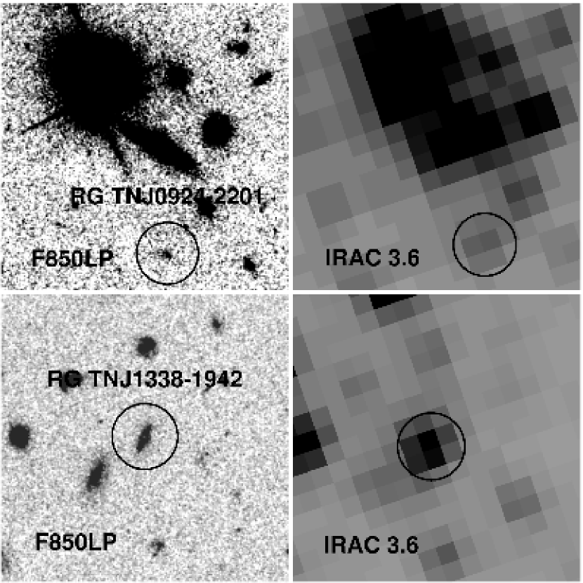
Figure 1.— Panels show the ACS $z_{850}$-band and IRAC 3.6$\mu$m images of the radio galaxies TN1338 at $z=4.1$ (bottom panels) and TN0924 at $z=5.2$ (top panels). The images measure 20″$\times$20″. The ACS images were convolved with a Gaussian kernel of $0\farcs 1$ (FWHM). The IRAC photometry was obtained by deblending the radio galaxies and their neighbouring sources using GALFIT (see §2 for details).

Follow-up infrared images for the fields TN0924 and SDSS0836 were obtained with the IRAC on the SST (PID 20749, Zheng 2006). We retrieved archival IRAC data of TN1338 (PID 17, Fazio 2004) and SDSS1030 (PID 30873, Labbé 2007). The IRAC camera includes imaging data at 3.6, 4.5, 5.8, and 8.0 $\mu$m (channels 1-4), each with a $5\farcm 2\times 5\farcm 2$ field and a pixel size of $\sim 1\farcs 22$. We concentrate here on the shortest-wavelength Spitzer image (channels 1 and 2) for the field at $z\sim 4$ (TN1338), and on the 3.6$\mu$m images for the higher redshift fields. The exposure times at 3.6µm are 17 ksec (TN0924 & SDSS0836) and 10 ksec (TN1338 & SDSS1030). For our photometry, we used the pipeline-processed IRAC images at the ‘post-basic calibrated data’ (PBCD) stage. The main steps in the pipeline include dark current subtraction, flat fielding, flux calibration (in units of MJy sr^-1), geometric distortion correction and mosaicking of the individual frames. Sensitivities of each image were estimated from the 2 $\sigma$ standard deviation in the flux distribution measured in randomly placed 3″ diameter apertures. The 2$\sigma$ limiting AB magnitudes are 25.5 (TN0924), 25.2 (J0836), 25.2 (TN1338), and 25.2 (J1030) mag in the 3.6 $\mu$m channel, and 25.0 (TN1338) and 24.6 (J1030) mag in the 4.5 $\mu$m channel.

2.5. IRAC Source Photometry using GALFIT

The IRAC images suffer from overcrowding due to its relatively large point spread function (PSF) of $\sim 1\farcs 5$ (FWHM) and great sensitivity. To address this issue, we use a deblending technique whereby contaminating neighbors are subtracted using GALFIT (Peng et al., 2002) by performing a fit to the objects of our interest and all their close neighbours simultaneously. GALFIT constructs a two-dimensional model of the data according to specified input parameters (e.g., positions, magnitude, effective radius, axis ratio, and position angle), performs a convolution with the instrument PSF, and fits the result to the data through an iterative $\chi^{2}$-minimization process. The IRAC PSF is obtained directly from the images by stacking 10 bright, isolated point sources. We use the higher resolution ACS $z$-band image as the reference for the initial GALFIT input parameters. GALFIT was then applied to the IRAC images. Two versions of the fitting process were carried out. First, all input parameters as determined from the $z$-band image were held fixed, except the magnitudes. The resulting $\chi^{2}$ value and residual image was then visually inspected to determine the goodness of fit. When the best possible fit was not achieved, we repeated the GALFIT procedure, but this time allowing all input parameters to vary. Each object was individually and interactively processed until the most successful fit was achieved, while avoiding the oversubtraction of the flux contribution from the neighboring sources. Following this, the two-dimensional models of the light profiles of the LBGs/LAEs and nearby contaminating sources were deblended. This deblending process works quite well for determining the intrinsic fluxes of most of LBGs/LAEs. Those sources for which GALFIT failed to satisfactorily deblend the emission of LBGs/LAEs from the neighbour sources were removed from the sample. This leaves a total of 60 sources (38 LBGs and three LAEs at $z\simeq 4.1$, 15 LBGs at $z\simeq 5.2$ and 4 LBGs at $z\sim 6$), for which reliable photometry from GALFIT was obtainable.

The measured 3.6 (4.5) $\mu$m magnitudes for the four fields are listed in Tables 1–4, along with the classifications of galaxies for their detections and degree of confusion, as (1) isolated and detected; (2) isolated but undetected; (3) confused (4) heavily blended. In Fig. 1 we show the ACS $z_{850}$ and IRAC 3.6$\mu$m images of the two bright radio galaxies for an illustration of the data quality and blending issues.

2.6. Emission line contamination corrections

Because the IRAC 3.6$\mu$m flux of the radio galaxy TN J1338–1942 is significantly contaminated by H$\alpha$ flux from its large emission line halo that is typical of RGs, we have used the emission-line free flux at 4.5$\mu$m and a small model extrapolation based on the typical [3.6]–[4.5] colors of star-forming galaxies at $z\approx 4$ to estimate the true continuum magnitude at 3.6$\mu$m as follows. The measured [3.6]–[4.5] color was –0.65 mag (see Table 1), while a comparison with stellar population models (see below) in 4.5$\mu$m vs. $z$–[4.5] space would predict a color of [3.6]–[4.5]$\sim$0–0.2 mag. We thus assume that H$\alpha$ contributes about $0.75\pm 0.10$ magnitude to the 3.6$\mu$m measurement of the radio galaxy, and we will apply the correction to all subsequent figures and tables. The 3.6$\mu$m flux of the radio galaxy TN J0924–2201 is not affected by H$\alpha$ given its higher redshift of $z=5.2$.

While the 3.6$\mu$m flux of $z\sim 4$ star-forming galaxies such as LBGs and LAEs is expected to have an enhancement due to H$\alpha$ as well, we do not correct for this effect as we can assume that galaxies in both GOODS and in the protocluster fields will be affected in a similar way. Stark et al. (2007) estimate that H$\alpha$ could in principle increase the broad band flux by $\sim 10-20$%.

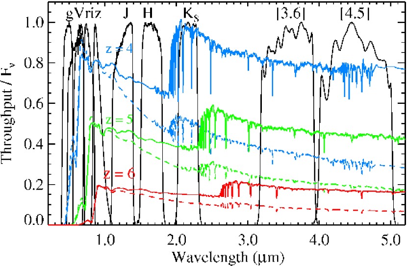
Figure 2.— Transmission curves of the relevant optical (HST/ACS), near-infrared, and infrared (IRAC) filters. We overplot several example spectral energy distributions modeled using BC03. Lines show the expectation for an exponentially declining star formation history with $\tau=100$ Myr at ages of 10 (dashed lines) and 100 Myr (solid lines), and redshifted to $z=4.1$ (blue lines), $z=5.2$ (green lines), and $z=6.0$ (red lines). A small attenuation of $E(B-V)=0.1$ magnitude was modeled using the prescription of Calzetti (2001) and applied to each of the tracks.

2.7. Estimating stellar masses

2.7.1 Rationale

In order to answer the question of whether there are any differences between the different types of galaxies across the CMD and across environment, we will seek to determine estimates of (primarily) stellar masses based on a set of $z$–[3.6] versus 3.6$\mu$m CMDs. Only recently has it become feasible to attempt an interpretation of the observed magnitudes of the relatively faint galaxy populations at $z\simeq 3-6$ in terms of stellar masses, ages, dust and star formation histories based on detailed fitting of SEDs using model libraries (see references given in §1 and therein). While there is ongoing debate about the correctness of the treatment of different stellar evolutionary phases in the model libraries (e.g. Fioc & Rocca-Volmerange, 1997; Bruzual & Charlot, 2003; Maraston et al., 2006; Rettura et al., 2006; Kannappan & Gawiser, 2007; Eminian et al., 2008), they at least allow for an assessment of the comparative properties among samples across redshift or across the CMD, provided that these samples are sufficiently ‘simple’ to model and that the adopting of a faulty model does not lead to catastrophic systematic effects across the various samples. At the least, this requires highly accurate photometry in all of the rest-UV, optical and infrared, and such studies have therefore been limited to a small set of well-studied fields.

While our ACS imaging is of comparable depth to, e.g., GOODS, we lack sufficiently deep data in the observed near-infrared. Our IRAC imaging provides a relatively good match to the ACS imaging (most UV-selected sources detected), but it is not as deep as some of the large field surveys. Therefore, we do not believe that a detailed SED fitting is warranted by our data, nor is it necessary for the limited questions we wish to ask. Instead, as we will show below, we can obtain sufficiently accurate information on stellar masses based on the comparison with simple baseline models rather than SED fitting (§2.7.2). We will test our method by making a comparison with the properties of mock galaxies selected in a large cosmological simulation (§2.7.3).

2.7.2 Comparison with Stellar Synthesis Models

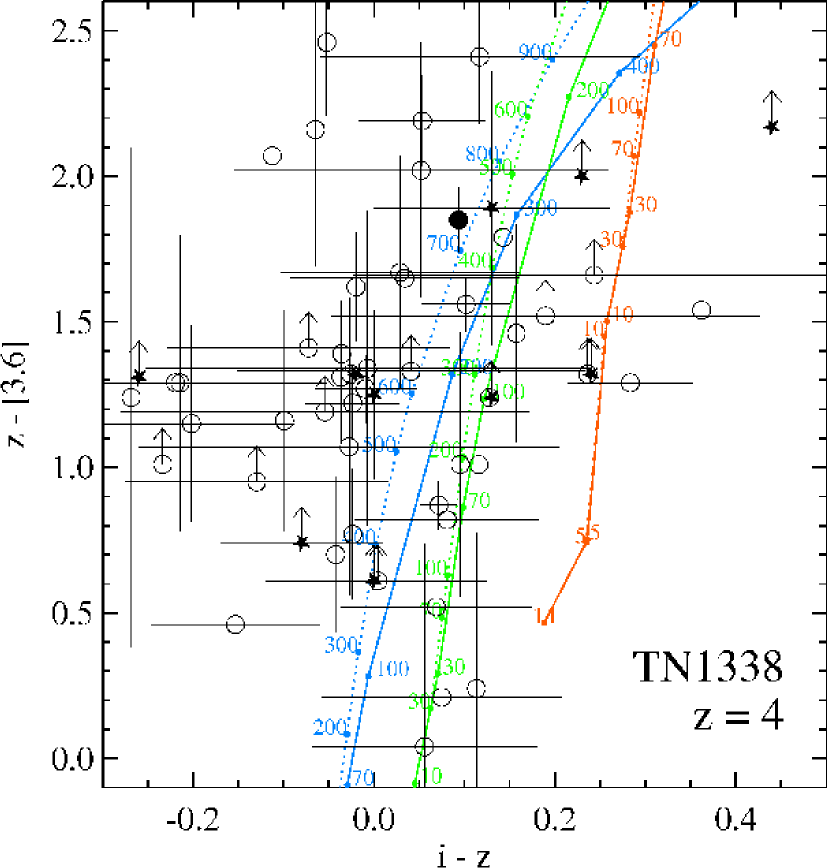
Figure 3.— The $i$–$z$ versus $z$–[3.6] color-color diagram for the TN1338 field. Symbols indicate the radio galaxy (large filled circle), LBGs (open circles) and LAEs (filled stars). Tracks indicate the colors of models having $\tau=30$ Myr (dotted lines) and $\tau=200$ Myr (solid lines) with ages in Myr indicated along the tracks. Attenuations of $E(B-V)=0.0,0.15,0.4$ mag are shown in blue, green and red, respectively. Most objects do not require a large amount of reddening due to dust.

As detailed in Stark et al. (2009), at $z\gtrsim 4$ the 3.6$\mu$m channel still probes only as red as the rest-frame optical, where the contribution from TP-AGB stars is much less severe than in the near-infrared. As a result, the stellar mass estimates based on “BC03” (Bruzual & Charlot, 2003) models are expected to be higher by at most $\simeq$30% when compared to the newer generation of models that include this phase (Bruzual, 2007), and the effect of AGB stars becomes less severe with increasing redshift and metallicity with respect to subsolar metallicity models at $z\sim 4$. Furthermore, the SED fitting appears to be relatively insensitive to whether redshifts are being fixed or allowed to vary within their $\Delta z=\pm 0.25$ uncertainty distributions typical for dropout samples.

In order to interpret the data in the CMDs that will be presented in §3, we have selected a set of BC03 models that we will use for a simple baseline comparison with our data. The models are based on the best-fit ages as obtained from pan-chromatic SED fits performed by Stark et al. (2009), and the typical attenuations due to dust as found by Bouwens et al. (2009). Both studies are based on large samples of dropout galaxies at $4\lesssim z\lesssim 6$ for which deep photometry is available. We choose an exponentially declining star formation history with an $e$-folding timescale $\tau$ of 100 Myr. We consider a range of ages from 100 to 300 Myr, straddling the best-fit age of $\sim$200 Myr as found by Stark et al. (2009). We will also consider three levels of attenuation by dust in terms of $E(B-V)=$0.0 mag (no dust), 0.15 mag (moderate extinction) and 0.3 magnitude (dusty), modeled using the recipes for starburst galaxies given in Calzetti (2001). All models have a metallicity similar to that of the Large Magellanic Cloud. We convert the models to the appropriate redshift, and calculate colors and magnitudes by convolving the spectral energy distributions with the HST and Spitzer filter transmission curves (Fig. 2). Given an age and an attenuation, an estimate for the stellar mass of each object is obtained by determining the absolute mass scale of the model required in order to reproduce the 3.6$\mu$m magnitude observed. Motivated by a recent study by Bouwens et al. (2009) that finds clear evidence of correlations between the UV color and absolute UV luminosity of $B$- and $V-$dropout galaxies, we will also investigate a model in which the dust and age are allowed to vary as a function of absolute magnitude.

These simple model comparisons show that while the 3.6$\mu$m magnitude is an approximate gauge of stellar mass at each of the redshifts, the $z$–[3.6] color is affected by significant degeneracies between age, dust and SFH that can only be satisfactorily addressed using deeper data and a wider set of bands than currently available for our fields. However, since this paper mainly focuses on general trends in stellar mass for different populations, our main results will not be significantly affected by this issue. Nonetheless, for the TN1338 field we can be a little more specific and try to get a better handle on the presence of dust. The $i$–$z$ UV continuum color reacts more strongly to reddening due to dust than the $z$–[3.6] color. This is illustrated in Fig. 3 where we show the TN1338 $i$–$z$ vs. $z$–[3.6] color-color diagram compared to models with three different attenuations of 0.0 (blue lines), 0.15 (green lines) and 0.4 mag (red lines). The symbols indicate LBGs (open circles), LAEs (filled stars), and the RG (filled circle). Most objects are very blue in the UV ($i$–$z\approx 0.0$ mag) implying a small amount of attenuation at most. In other words, strongly reddened galaxies do not appear to make an important contribution. This is not surprising since not only is our UV selection biased against very dusty objects, recent evidence suggests that dusty objects become increasingly rare at $z\gtrsim 4$ (e.g. McLure et al., 2006; Stark et al., 2009; Bouwens et al., 2009, Sect. 4.4 of this paper).

2.7.3 Comparison with Mock Galaxies in the Millennium Run Simulations

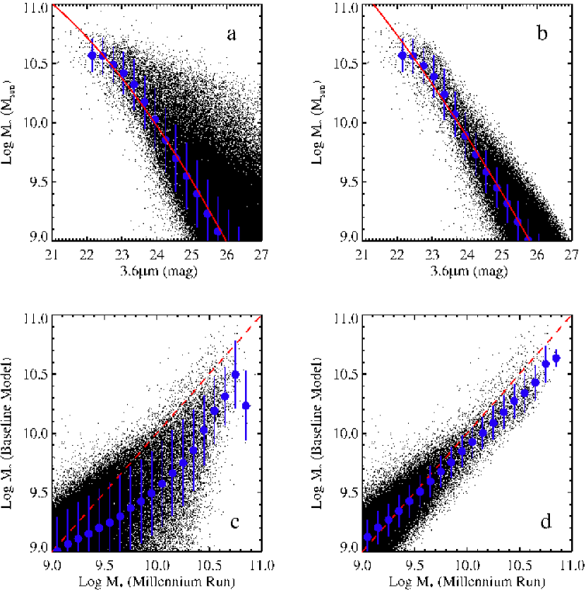
Figure 4.— The accuracy of our method of retrieving stellar masses based on simple SED assumptions, tested against one million mock galaxies selected from the Millennium Run (MR) cosmological simulations. Top panels show the relation between stellar masses and 3.6$\mu$m magnitudes for the entire MR sample (panel a, left) and for a cleaned subset of galaxies most similar to our UV-selected samples (panel b, right). Blue points indicate the median values and the 1$\sigma$ standard deviation in bins of $\Delta m=0.3$ mag. A second-order polynomial fit to the correlation shown in panel b is $\mathrm{log}M_{*}[M_{\odot}]=11.51+0.32m_{3.6}-0.016m_{3.6}^{2}$ (red line). In the bottom panels, we demonstrate how accurately we can derive the true stellar masses from the observed 3.6$\mu$m magnitudes under the assumption of a fixed baseline SED characterized by $\tau=100$ Myr, $t=200$ Myr, $E(B-V)=0.15$ mag, and LMC metallicity. Despite the inevitable mismatches between the baseline model and the true properties of the simulated galaxies, there is still a very good correlation between the true mass and the mass inferred using the baseline model. The one-to-one correlation is indicated by the red dashed lines. There is a small systematic offset in the sense that for more massive galaxies we underestimate their true mass based on the baseline SED model (by about $\sim$0.3 dex at $M_{*}\sim 10^{11}$ $M_{\odot}$, see panel d for the sample most similar to our UV selection).

Above we have outlined our basic strategy of using simple baseline models to convert 3.6$\mu$m fluxes into stellar mass estimates. In order to test this we use our large sample of mock galaxies from the Millennium Run simulations (see Sect. 2.3). In the top-left panel of Fig. 4 (panel a) we plot the stellar mass against the observed-frame 3.6$\mu$m magnitude for each of the mock galaxies at $z=4$. The 3.6$\mu$m magnitude is clearly correlated with the stellar mass, indicating that the flux at rest-frame $\sim$7000Å is a good tracer of the mass. Next, we limit the mock sample to only those galaxies that are most similar to the galaxies in our UV-selected LBG samples by requiring relatively little dust ($E(B-V)<0.3$ mag, see Fig. 3) and current star formation activity at a rate of $>$1 $M_{\odot}$ yr^-1. The result is shown in the top-right panel (b). The scatter around the correlation between $M_{*}$ and 3.6$\mu$m is significantly reduced. We see that a range in the 3.6$\mu$m magnitude from 26 to 21 mag corresponds to a range in stellar mass from $10^{9}$ to $10^{11}$ $M_{\odot}$. A second-order polynomial fit to the data yields $\mathrm{log}M_{*}[M_{\odot}]=11.51+0.32m_{3.6}-0.016m_{3.6}^{2}$ (red line in panel b)

As stated earlier there are ambiguities between SFH, age and dust that cannot be solved for based on our current data. However, we can also use the MR simulations to test how well we can retrieve stellar masses when assuming that each galaxy can be approximated by a single one of our simple baseline SEDs from Sect. 2.7.2 (e.g., $\tau=100$ Myr, $t=200$ Myr, $E(B-V)=0.15$ mag) for each 3.6$\mu$m magnitude. The result is shown in the bottom panels of Fig. 4, again for all (left panel, c) and for the “cleaned” subsample (right panel, d). Despite the inevitable mismatches between the baseline model and the true properties of the simulated galaxies, there is a very good correlation between the true mass and the mass inferred using the baseline model. We do however see a systematic offset in the sense that for more massive galaxies we underestimate their true mass based on the baseline SED model (by about $\sim$0.3 dex at $M_{*}\sim 10^{11}$ $M_{\odot}$). This can be understood because more massive objects have higher SFRs and have more dust in the simulations. Therefore, they also will have more dust compared to our baseline model so their 3.6$\mu$m flux is lower and hence we get a lower mass using the baseline model conversion.

The results obtained for our $z=5$ sample are very similar, but are not shown here for brevity. In summary, these simulations demonstrate that our approach of using simple baseline models to infer stellar masses from the 3.6$\mu$m data is justified.

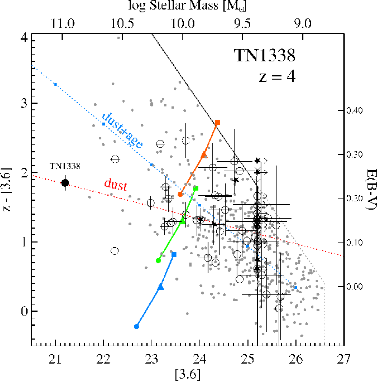
Figure 5.— The 3.6$\mu$m versus $z$–[3.6] color-magnitude diagram for galaxies in the field TN1338. Symbols indicate the radio galaxy (large filled circle), LBGs (open circles) and LAEs (filled stars). The 3.6$\mu$m flux of the radio galaxy has been corrected for H$\alpha$ emission line contamination (see §2.6). The $B_{435}$-dropouts from Stark et al. (2009) are shown for comparison (small grey circles). The approximate detection limits for the TN1338 field and the GOODS control field are indicated by the black solid and grey dotted lines, respectively. The colored solid lines indicate our BC03 baseline SED models described in §2.7.2, i.e. exponentially declining SFHs ($\tau=100$ Myr) having attenuations of $E(B-V)=0.0$ (blue), 0.15 mag (green) and 0.3 mag (red), each plotted at ages of 100 (circle), 200 (triangle) and 300 Myr (square). The models were normalized to a total stellar mass of $10^{10}$ M_⊙. The right and top axes, respectively, show the attenuation and stellar mass obtained for a model having a fixed age of 200 Myr (for $M_{*}$ we fix $E(B-V)$ to 0.15). The red dotted line (marked ‘dust’) indicates the minimum color change as a function of 3.6$\mu$m magnitude that is expected purely due to dust based on the $M_{UV}$ vs. $E(B-V)$ relation found by Bouwens et al. (2009) (and further assuming $\tau=100$, $t=200$ Myr in order to predict the $z$–[3.6] color). The blue dotted line (marked ‘dust$+$age’) indicates a toy model in which we let both the dust and age increase in steps of $\Delta E(B-V)=0.05$ and $\Delta t=50$ Myr with decreasing 3.6$\mu$m magnitude starting from $E(B-V)=0.0$ and $t=200$ Myr (each step is indicated by a small blue square). The latter model (‘dust$+$age’) is at least qualitatively in better agreement with the relatively steep change in color as a function of the 3.6$\mu$m magnitude compared to the ‘dust only’ model.

3. RESULTS

In this Section, we present the 3.6$\mu$m versus $z$–[3.6], or rest-frame UV-optical, color-magnitude diagrams (CMDs) of the various galaxy populations detected in the RG and QSO fields. We derive the stellar masses of LBGs, LAEs and radio galaxies, and perform a comparison between the samples in overdense regions and in the (GOODS) field.

3.1. UV-optical Color-Magnitude Diagrams in RG Fields at $z\simeq 4-5$

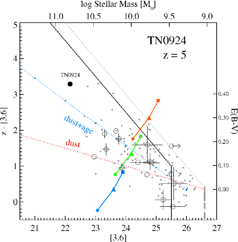
Figure 6.— The 3.6$\mu$m versus $z$–[3.6] color-magnitude diagram for galaxies in the field TN0924. Symbols indicate the radio galaxy (large filled circle) and LBGs (open circles). The $V_{606}$-dropouts from Stark et al. (2009) are shown for comparison (small grey circles). The approximate detection limits for the TN0924 field and the GOODS control field are indicated by the black solid and grey dotted lines, respectively. The baseline SED model tracks are shown for $z\simeq 5$ but are otherwise identical to the models in Fig. 5 (see caption of Fig. 5 for details). The right and top axes, respectively, show the attenuation and stellar mass obtained for a model having a fixed age of 200 Myr (for $M_{*}$ we fix $E(B-V)$ to 0.15). The red dotted line (marked ‘dust’) indicates the minimum color change as a function of 3.6$\mu$m magnitude that is expected purely due to dust based on the $M_{UV}$ vs. $E(B-V)$ relation found by Bouwens et al. (2009) for $z\sim 5$. The blue dotted line (marked ‘dust$+$age’) indicates a toy model in which we let both the dust and age increase in steps of $\Delta E(B-V)=0.05$ and $\Delta t=50$ Myr with decreasing 3.6$\mu$m magnitude starting from $E(B-V)=0.0$ and $t=200$ Myr (each step is indicated by a small blue square).

In Fig. 5 we show the 3.6$\mu$m versus $z$–[3.6] diagram for our samples of galaxies at $z\simeq 4.1$ in the field TN1338. Symbols indicate the $g$-dropouts (open circles), the LAEs (stars), and the radio galaxy (large filled circle). Two LAEs were unfortunately confused beyond the possibility of deblending. Of the remaining 10 LAEs, only three were detected at 3.6$\mu$m and we derive limits for the seven that were undetected. Also in Fig. 5, we show the distribution of $z\sim 4$ $B_{435}$-band ($B$) dropouts from GOODS (grey circles) as selected by Stark et al. (2009) for comparison.

Next, in Fig. 6 we present the CMD of the $V$-dropouts (open circles) and the radio galaxy (filled circle) at $z\simeq 5.2$ in the field TN0924. Unfortunately, three out of four of the LAEs in this field suffered from a large amount of confusion, and no attempt was made for photometry. One LAE was found to be relatively isolated but not detected. Again, for comparison with the field we indicate a large number of $V$-dropouts from GOODS using grey circles.

A number of basic observations from these diagrams can be made:

(1) Our dropout samples show a sequence in the CMD with a total width in color of $\sim 2$ magnitude and a total range in 3.6$\mu$m of four magnitudes ($\sim$22–26 mag), peaking at $3.6\mu m\sim 25$ and $z$–[3.6]$\sim 1$. While the upper envelope in both CMDs is largely set by the limiting $z$-band magnitude by which the samples were selected (dashed lines in Figs. 5 and 6), the lower envelope is physical in the sense that brighter objects (at 3.6$\mu$m) are also redder. The same trend is seen for the GOODS reference samples (grey circles), indicating that it is a general feature of the high redshift population.

(2) The LAEs in the TN1338 field, the only field with a sufficiently large sample available for attempting photometry by means of deblending (see §2), mostly show non-detections at 3.6$\mu$m. The three detected LAEs were L9, L16 and L22 (see Overzier et al., 2008). L9 is also part of the LBG sample, while L16 and L22 are respectively too blue or too faint to make it into our $g$-dropout LBG sample. These results were expected given that about half of the LAEs are fainter than $z_{850}$=26.5 magnitude in the rest-frame UV and the rather linear correlation between the rest-UV and optical in the CMD. In any case we can conclude that we have not found any LAEs that are particularly bright or red compared to the LBGs, although we should note that the RG has an extremely luminous associated Ly$\alpha$ halo typical of radio galaxies that would formally put it into a Ly$\alpha$-selected sample as well.

(3) Both radio galaxies have extraordinarily bright rest-frame optical magnitudes, at least one magnitude brighter than the brightest LBG and 2–4 magnitudes brighter at 3.6$\mu$m compared to the bulk of the LBG populations at $z\sim 4$ and $z\sim 5$. They also have relatively red UV-optical colors but perhaps not redder than the extrapolated color of the sequence formed by LBGs at lower magnitudes.

3.2. Mass Segregation of LAEs, LBGs and Radio Galaxies

As explained in §2.7.2 we use a limited set of spectral energy distributions as simple baseline models for interpreting the CMDs shown in Figs. 5 and 6. In these figures we have indicated the expected location of star-forming galaxies with exponentially declining star formation histories of $\tau\approx 100$ Myr, dust attenuations in terms of $E(B-V)$ of 0.0 (blue lines), 0.15 (green lines) and 0.3 mag (red lines) modeled using the recipes for starburst galaxies given in Calzetti (2001), and plotted at three ages of 100, 200 and 300 Myr (indicated by the circle, triangle and square, respectively). The tracks were normalized to a total stellar mass of $10^{10}$ M_⊙. These models span an appropriate range of parameter space compared to the detailed investigations of Stark et al. (e.g. 2007, 2009, and references therein) and Bouwens et al. (2009). The right and top axes of Figs. 5 and 6 show the attenuation and stellar mass obtained for a model having a fixed age of 200 Myr.

3.2.1 RGs

At $z=4.1$ and $z=5.2$, the 3.6$\mu$m band probes the rest-optical at $\sim$7000 and 6000Å, respectively. At these wavelengths, the light is believed to be largely stellar in origin (Zirm et al., 2003; Seymour et al., 2007), despite the many significant, non-stellar components of radio galaxies across the entire spectrum. In both fields, we find that the RG is the most massive object, with an inferred mass of $\sim$ $10^{11}$ M_⊙. Without more constraints on the SED we judge that this estimate can be higher or lower by $\sim$25% depending on the exact age and attenuation. TN0924 at $z=5.2$ is over a magnitude redder than TN1338 at $z=4.1$. If the attenuations are similar, it implies that the higher redshift RG is about twice as old as the lower one ($\sim$600 vs. 300 Myr). In any case, it is interesting that both RGs are much more massive than any of the LBGs in their surrounding fields.

3.2.2 LBGs

We now compare the dropouts with the model tracks plotted in Figs. 5 and 6. In both RG fields we find that the range in 3.6$\mu$m magnitude of the $g$-dropout and $V$-dropout LBGs implies a distribution in stellar mass of about one order of magnitude, from a few times $10^{9}$ to a few times $10^{10}$ M_⊙. The CMD slope can be explained entirely by a correlation between dust and stellar mass, finding ages of $\sim 100-200$ Myr and dust increasing from $\sim 0.0$ to $\sim$0.15 mag between the low and high mass end. Alternatively, interpreting the CMD slope as an age effect, the low mass end objects are consistent with an age of $\sim$70–200 Myr and small attenuation, while the typical age at the high mass end would be $\sim 2.5\times$ higher ($\sim 200-500$ Myr) for a similar attenuation. We will discuss the age-dust (and metallicity) degeneracy in more detail in Sect. 3.3 below.

3.2.3 LAEs

Due to the non-detections and overall small number of LAEs in the TN0924 field, we can only compare LAEs and LBGs in the TN1338 field. Most of LAEs were undetected, suggesting masses of $\lesssim 10^{9}$ M_⊙, and we note that many of the faintest LBGs were undetected as well. The brighter, detected LAEs have colors that are consistent with those of non-Ly$\alpha$ LBGs at similar optical magnitudes. The tendency of LAEs at $z\sim 4$ to be relatively faint and blue in the rest-frame UV/optical is consistent with their young age as found in other surveys (e.g. Shapley et al., 2003; Gawiser et al., 2006; Pentericci et al., 2007, 2009; Ouchi et al., 2008) and predicted by some simulations (Nagamine et al., 2008).

3.3. Interpreting the relation between $M_{*}$ and $z$–[3.6] color

In Figs. 5 and 6 we have observed a strong trend of redder $z$–[3.6] colors with increasing stellar mass. This trend is qualitatively similar to the “blue envelope” of LBGs at $z\sim 3-4$ observed by Papovich et al. (2004) and must be related to an increase in the mean age, dust or metallicity (or a combination thereof) with increasing rest-frame optical luminosity. While we cannot solve these degeneracies on an object-by-object basis without deep multi-wavelength photometry, we can use recent results from literature to explain the general trends observed. Deep studies of dropouts covering a wide range in both redshift and UV luminosity have now clearly demonstrated that star-forming galaxies become bluer in the UV continuum with increasing redshift and with decreasing luminosity (Papovich et al., 2004; Stanway et al., 2005; Hathi et al., 2008; Bouwens et al., 2009), in some contrast with earlier results that indicated no clear correlation between the slope of the UV continuum and UV luminosity (e.g. Meurer et al., 1999; Adelberger & Steidel, 2000; Ouchi et al., 2004). As shown by Bouwens et al. (2009), these results can be fully explained by the relatively limited range in redshift and/or UV luminosity probed by earlier surveys. Using the deepest data available from the Hubble Ultra Deep Field (UDF; Beckwith et al., 2006), these authors show that there is a significant correlation between the UV slope and the UV luminosity for both $B$- and $V$-dropouts. They also investigate the relative effects that, in principle, metallicity, age and dust each could have on the observed UV slope. They find that both dust and age have the potential of reddening the UV continuum significantly, with the effect of dust being the strongest for realistic distributions of age and dust. The influence of metallicity is found to be only small.

Could the trends that we found in Figs. 5 and 6 be explained due to systematic changes in dust and age with increasing stellar mass (or 3.6$\mu$m luminosity)? Stark et al. (2009) have shown that the median ages of dropouts at $4<z<6$ (the same samples that we have used for our comparison) change only little with either redshift or UV luminosity (less than a factor of 2). However, they do find a strong correlation between stellar mass and SFR as inferred from the UV continuum luminosity (with a net specific SFR, SFR/$M_{*}$, that is relatively constant as a function of stellar mass). The correlation between SFR and extinction by dust is well-known, as galaxies with higher SFRs tend to have more dust (e.g. Wang & Heckman, 1996; Martin et al., 2005; Reddy et al., 2006). Bouwens et al. (2009) have now firmly established this correlation for LBGs by studying the average UV color (a measure of reddening) as a function of the absolute UV magnitude (a measure of the unextincted SFR). As argued by Bouwens et al. (2009), we thus expect to see a strong correlation between stellar mass and reddening due to dust. In Figs. 5 and 6 we have indicated the expected amount of reddening purely due to dust based on the empirical UDF results. In both figures, the red dotted line marked ‘dust’ indicates the color change (as a function of 3.6$\mu$m magnitude) expected based on the relation between $M_{UV}$ vs. $E(B-V)$ from Bouwens et al. (2009, see their Fig. 3). Using this relation, the extinction varies from $E(B-V)\approx$0.0 to $\approx$0.2 mag from the faint to the bright end. While the trend predicted by our UV-to-($z$–[3.6]) color extrapolation shows the correct general behavior, the reddening in $z$–[3.6] expected seems to underpredict the amount of reddening observed. This may indicate that, besides the increased reddening due to dust, additional reddening is required due to age as a function of stellar mass.

To illustrate this further we construct a simple toy model. We let both dust and age increase towards brighter 3.6$\mu$m magnitudes. The $E(B-V)$ is increased in steps of 0.05 and the age in steps of 50 Myr. The resulting color trend for this toy model is shown by the blue dotted line marked ‘dust$+$age’ in Figs. 5 and 6. The starting point (marked by the small blue square on the faint end of the blue dotted line) was chosen to have $E(B-V)=0.0$ and an age of 200 Myr. The ‘dust$+$age’ model is, at least qualitatively, in better agreement with the relatively steep change in color as a function of the 3.6$\mu$m magnitude compared to the ‘dust’-only model.

In principle, it should be possible to find the required evolution in dust and age that best fits the general trends observed in the CMDs. However, Figs. 5 and 6 show that the dynamic range in $z$–[3.6] color in the TN1338, TN0924 and GOODS fields is too small to carry out such an exercise (i.e., a fit to the data can not be made due to relatively red sources being missed at the faint end). Deeper data in the rest-frame UV would greatly alleviate this problem, and it should be possible to perform such a study in the much deeper UDF.

3.4. Comparison of galaxies in overdense regions versus galaxies in average environments from GOODS

It has previously been shown that the number density of dropouts and LAEs in the TN1338 and TN0924 fields is larger relative to random fields, indicating that these fields may host massive galaxy clusters-in-formation (Venemans et al., 2002, 2004; Overzier et al., 2006, 2008). One of the goals of the current paper was to test whether besides this enhancement in number density there also exist differences in the physical properties of galaxies in overdense regions compared to the field. The large samples of $B$- and $V$-dropouts extracted from the $\sim 320$ arcmin² GOODS field by Stark et al. (2009) allow us to make such a comparison. Comparing the color-magnitude distribution in our fields with the results found for GOODS (grey circles in Figs. 5 and 6) indicates a very similar trend of redder colors for brighter objects. This suggests that, at least at first sight, in both types of environment the dropout populations as a whole possess very similar stellar populations.

Unfortunately, there are several factors that complicate making further quantitative statements about the differences or similarities between overdense fields and GOODS. First, the size of the individual error bars in the CMD diagrams is substantial, thereby limiting the usefulness of object-by-object comparisons except for the brightest objects (as we will see below). Second, because we only have limited filters and miss deep NIR data, an analysis based on multi-band SED fitting is not yet possible for our fields. Third, although many of the dropout galaxies are believed to be associated with the protoclusters in the vicinity of the radio galaxies, we must note that the dropouts in TN1338/TN0924 are not spectroscopically confirmed, except for the subset that are Ly$\alpha$-bright. This means that our dropout samples will undoubtedly include galaxies in the (near) fore- and background of the protoclusters that could offset or bias any trends observed in Figs. 5 and 6.

These caveats aside, however, we can at least ask the question what differences with GOODS we would in principle be able to detect based on the quality of our data presented. The first possibility we consider is that if galaxies in the overdense regions were systematically bluer or redder compared to the field, the protocluster dropouts may be expected to form a lower or upper envelope with respect to the well-established CMD slope formed by the GOODS dropouts at $z\simeq 4-5$. We estimate that a systematic difference in ages by a factor of $\gtrsim 2$ or a difference in attenuation of $\gtrsim 0.15$ mag would have been detectable given the size of the error bars in Fig. 5. However, no such differences are suggested by the data.

Another possibility we consider concerns the hypothesis that the overdense regions contain more massive galaxies compared to the general field. In this scenario, we would expect an extension towards brighter 3.6$\mu$m magnitudes (larger stellar masses) relative to GOODS. Because every object in the overdense region would become a little brighter, this means that at the faint end of the luminosity/mass function more objects in the overdense region would pass the detection threshold, while the number for the “field” would remain the same. Therefore, one would not immediately expect to find any differences between the average properties of galaxies at the faint end. At the bright end, however, one would expect an excess of massive sources relative to the field. We estimate that a boost in masses by a factor of a few should be detectable in the CMD diagrams. In this respect, it is interesting that in both fields, the RGs are brighter than any dropout from the GOODS comparison sample, even though the latter survey covers an area that is over 25 times larger. We have also analyzed the relative numbers of dropouts in the fainter magnitude bins, finding no evidence for a significant brightening of dropouts in the overdense regions. From this it follows that compared to GOODS the protocluster fields likely do not contain an excessive number of bright/massive ($\sim 10^{11}$ $M_{\odot}$) LBGs other than the radio galaxies themselves. We will further discuss these results in §4.

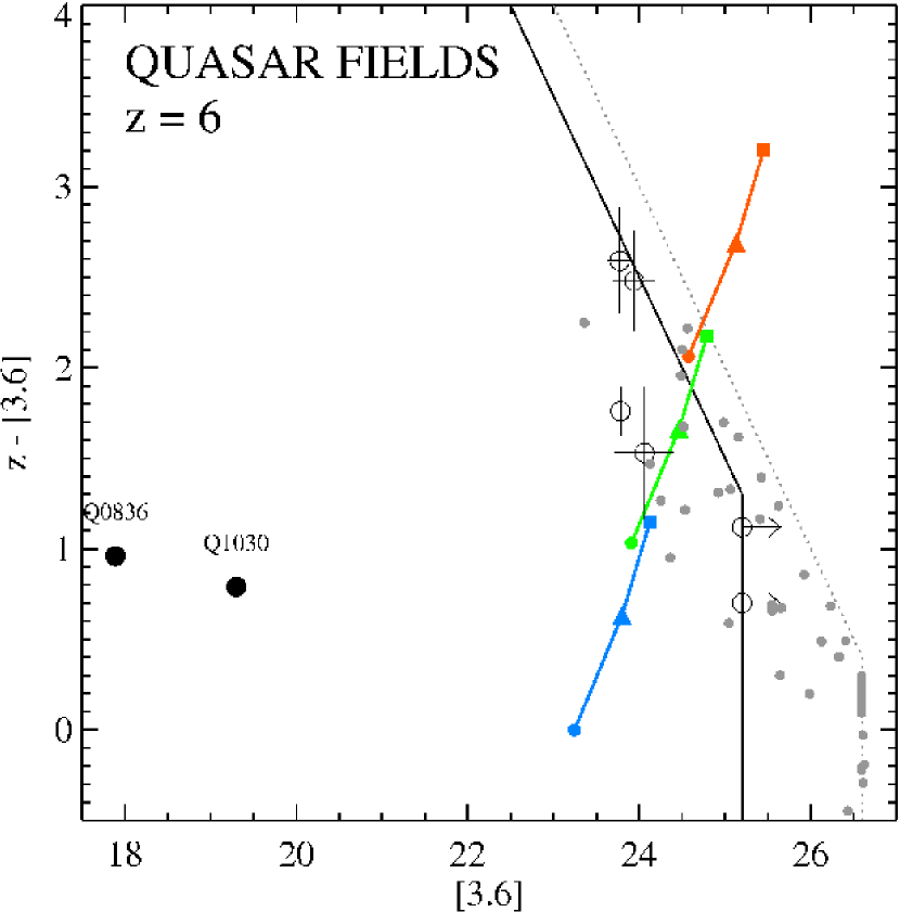
Figure 7.— 3.6$\mu$m versus $z$–[3.6] color-magnitude diagram for the $z\simeq 6$ $i_{775}$-dropouts selected from the fields SDSS0836 (QSO at $z=5.82$) and SDSS1030 (QSO at $z=6.28$). Symbols indicate the quasars (large filled circles) and $i_{775}$-dropouts (open circles). The $i_{775}$-dropouts from Stark et al. (2009) are shown for comparison (small grey circles). The approximate detection limits for the QSO fields and the GOODS control field are indicated by the black solid and grey dotted lines, respectively. Model tracks have been indicated for $z\simeq 6$ but are otherwise identical to the ones shown in Figs. 5 and Fig. 6 (see the caption of Fig. 5 for details). The QSOs have been indicated for reference only, as their magnitude and colors are completely dominated by AGN light instead of stellar light.

3.5. UV-optical Photometry of $i$-dropouts in Two QSO Fields at $z\simeq 6$

For completeness, we will use our ACS and IRAC data on the two $z\sim 6$ QSO fields in order to perform a similar analysis for the $i$-dropout candidates in the (projected) vicinity of the luminous quasars. We have tabulated our measurements in Table 4 and plot the CMD in Fig. 7. We also plot the QSOs in the CMD but stress that their emission is strictly dominated by non-stellar processes and should not be compared with any other populations or models shown in this paper. We compare our results again with a small sample of similarly selected $i$-dropouts from GOODS (grey circles), and with the same model tracks as plotted in Figs. 5 and 6. The colors of the four $i$-dropouts in the QSO fields that are detected in both bands are clearly inconsistent with very young, dust-free models (e.g. the blue track in Fig. 7), while the masses are on the order of $10^{10}$ M_⊙ relatively independent of dust and age. The faintest objects that can be probed in GOODS are about ten times less massive due to the much higher sensitivity in the [3.6] channel (Yan et al., 2005; Stark et al., 2007). Comparing the two distributions further suggests an excess of sources having 3.6$\mu$m$<$24.5 magnitude in the QSO fields not seen in GOODS. Unfortunately, the small number statistics, the uncertainties in the redshifts and the photometric errors do not allow us to say at present whether this trend is real or not.

4. SUMMARY AND DISCUSSION

4.1. Summary

Summarizing our results from the previous section, at $z\simeq 4.1$, the masses and stellar populations of RGs and LBGs are found to lie in a similar range as those at $z\simeq 5.2$, with the RGs being systematically the most massive objects ($\sim 10^{11}$ $M_{\odot}$). The stellar mass of the LBGs ranges from a few times $10^{9}$ to a few times $10^{10}$ M_⊙, and there is a clear trend of redder colors with increasing mass. The correlation can be explained if more massive galaxies have more dust (because their SFR is higher) and are somewhat older compared to less massive galaxies. Few LAEs were detected, implying they are generally of low mass. The RGs, LBGs and perhaps LAEs thus appear to be on different evolutionary tracks with the RGs having experienced either a more prolonged or more efficient phase of star formation history compared to LBGs, and LAEs being on average in earlier stages than the typical UV-selected LBGs in these fields (but perhaps not different compared to LBGs of the same UV luminosity!). We investigated possible differences between the properties of galaxies in overdense regions and those of dropouts from the much larger GOODS survey based on the distribution of objects in the rest-frame UV-optical CMD diagram. We found no significant, systematic differences between the overall distributions in $z$–[3.6] color and 3.6$\mu$m magnitude between dropout galaxies in the different regions. We did however find that in both fields the stellar masses of the radio galaxies as inferred from the 3.6$\mu$m flux are highly excessive compared to the general field expectations from GOODS. The latter survey virtually contains no dropout galaxies as bright (at 3.6$\mu$m) as the RGs, even though the area surveyed by GOODS is about 25$\times$ larger. Their (inferred) stellar masses of $\sim 10^{11}$M_⊙ are also about an order of magnitude larger than the brightest LBGs in the protocluster fields.

4.2. The most massive galaxies at $z\simeq 4-5$

Even though we have shown that none of the objects in GOODS are as bright as the RGs, Stark et al. (2009) find a non-negligible number of objects having comparable masses based on the detailed SED fits performed for GOODS. Thus, for the first time, we have a quantitative number density of massive galaxies from the field to be compared with RGs and protocluster regions. In order to quantify how rare galaxies with stellar masses as high as observed for the RGs are, we use the total number densities of (UV-selected) galaxies having stellar masses $>10^{11}$ M_⊙ as derived by Stark et al. (2009). They find number densities of $N(>M)\sim 6\times 10^{-6}-4\times 10^{-5}$ Mpc^-3 at $z\sim 4$ and $N(>M)\sim 1\times 10^{-6}-2\times 10^{-5}$ Mpc^-3 at $z\sim 5$ (ranges are 1$\sigma$), and we note that the upper values on these number densities are perhaps overestimated as non-spectroscopically confirmed sources having $z$–[3.6]$\gtrsim 2$ may have some contamination from dusty star-forming systems at $z\simeq 2$ (Yan et al., 2004; Stark et al., 2009).

The co-moving volumes of the TN1338 and TN0924 fields are $\approx 2\times 10^{4}$ Mpc³ (Overzier et al., 2006, 2008), implying that we would naively expect as many as, respectively, 0.1–0.8 (0.1–0.6 if we assume that the 24$\mu$m-detected objects in GOODS are foreground contamination) and 0.02–0.4 highly massive galaxies in a random single ACS pointing. Thus, it appears that the presence of a single $\sim 10^{11}$ M_⊙ (radio) galaxy in the protocluster fields is marginally consistent with the ($1\sigma$) upper limits on the cosmic average number density at $z\simeq 4$ while it is a positive deviation of several sigma at $z\simeq 5$. The GOODS field estimates are about two times higher than the values derived by McLure et al. (2008) based on a much larger survey of 0.6 deg², indicating that the GOODS estimates are probably not missing a significant fraction of massive (UV-selected) objects. Furthermore, to date no objects have been found with masses in excess of a few times $10^{11}$ M_⊙. Our results thus confirm earlier studies that suggest that RGs are among the most massive galaxies in the early Universe (e.g. Pentericci et al., 1997; Seymour et al., 2007, and see Fig. 5 in Rocca-Volmerange et al. (2004)). The low average number density of such objects further implies that the RGs in the TN1338 and TN0924 fields have experienced a rapid growth through accretion of gas or merging, presumably as a consequence of their overdense environments. This is qualitatively consistent with some models that specifically require an extra bias factor due to mergers in order to explain the strong clustering of luminous quasars at $z\sim 4$ (e.g. Wyithe & Loeb, 2009).

From the lack of any known bright radio sources among the massive GOODS galaxies (see Mainieri et al., 2008, for details on a radio follow-up in the GOODS-CDFS), we can deduce that if a powerful (radio) AGN is a typical phase of massive galaxies at $z\simeq 4-5$, then it is unlikely to last longer than 30–50 Myr. Otherwise, radio galaxies would be quite common in a field the size of GOODS given that the $B$-dropout ($V$-dropout) samples span $\sim$500 ($\sim$300) Myr in look-back time. This simple estimate based on the number counts is quite close to the expected radio source life-times of $\sim$10 Myr derived using other arguments (Blundell & Rawlings, 1999). If, on the other hand, none of the massive GOODS galaxies become radio galaxies even for a brief period during the epoch at $z\simeq 4-5$, it may mean that additional requirements for producing them must be met. Perhaps the overdense environment as observed in the protocluster fields TN1338 and TN0924 facilitates the rapid accretion of cold gas through mergers or cosmological flows (Kereš et al., 2009) spawning both a massive starburst and powerful AGN activity of a supermassive black hole (see Zirm et al., 2005, 2009).

4.3. Relation to low redshift clusters

Stark et al. (2009) compared the number density of $\gtrsim 10^{11}$ M_⊙ $B-$ and $V$-dropout systems to the observed density of quiescent $\sim 10^{11}$ M_⊙ galaxies at $z\sim 2.5$, finding that the high redshift sample can account for $\sim 20$% of the massive population at lower redshift. In a similar fashion, we can compare the number density of the most massive objects in GOODS at these redshifts to the number density of galaxy clusters in the local Universe, finding that they are roughly equal for clusters having $L_{X}\sim 1-5\times 10^{43}$ erg s^-1 (Rosati et al., 1998). Thus, one may expect that the $z=0$ descendants of the most massive $z\sim 4$ galaxies in GOODS are found in typical group and cluster environments (see also Ouchi et al., 2004). Since the radio galaxy fields studied in this paper are overdense with respect to GOODS, it will be interesting to perform a systematic study of galaxies in the direct environment of the massive GOODS galaxies (e.g. Daddi et al., 2009).

We have argued that the overdense regions correspond to sites of massive cluster formation. If so, we expect that the protocluster region will start to develop a cluster red sequence and a virialized intracluster medium at some redshift $z\lesssim 2$. Likely, the stars formed in the protocluster galaxies observed at $z\simeq 4-5$ will evolve and become incorporated into the population of massive early-type galaxies on the red sequence. We can use our results of §3 to estimate what fraction of this low redshift cluster red sequence mass is represented by all protocluster galaxies detected. We use the conversion between 3.6$\mu$m magnitude and $M_{*}$ derived from the simulations in §2.7.3 and calculate the total mass of all dropouts in the TN1338 field at $z=4$. We find a total stellar mass of $\sim 5\times 10^{11}$ $M_{\odot}$. About 25% of this mass is due to the large contribution from the radio galaxy.

We will now compare our estimate to the total stellar mass on the red sequence of the cluster RDCS1252.9–2927 (Cl1252), a massive X-ray luminous cluster at $z=1.24$ (Blakeslee et al., 2003a; Rosati et al., 2004; Demarco et al., 2007). Although we do not necessarily expect that TN1338 will evolve into a similar cluster as Cl1252 (see discussion below), we choose this particular cluster for our demonstration for a number of reasons. First, the analysis of Cl1252 was performed by members of our team, giving a good understanding of the data and its interpretation. More importantly, it is one of the best studied high redshift clusters, and its high redshift ensures a minimal gap in cosmic time with respect to $z=4$ (about 3.5 Gyr). This is important because below we will perform a simple extrapolation of the stellar masses measured at $z\sim 1$ to those predicted at $z=4$.

The analysis of Cl1252 performed by Rettura et al. (2008) found that 80% of the ETGs have population ages of $3.5\pm 1$ Gyr, consistent with a mean formation redshift of $z\sim 4$. If we limit ourselves to ETGs for which the mean star formation weighted ages are $>3.5$ Gyr, we find 10 massive ($M_{*}\gtrsim 10^{11}$ $M_{\odot}$) early-type galaxies (ETGs) representing a total “red sequence mass” of $3.5\times 10^{12}$ $M_{\odot}$ (about half of which is due to the three most massive ETGs). If we now assume that all the dropouts detected in the TN1338 field are part of the protocluster, its total stellar mass amounts to about 14% (at most) of the total Cl1252 ETG mass presumed to have formed at $z\gtrsim 4$. This percentage (14%) implies that we are currently missing most of the mass that we naively expected to have existed already at $z\sim 4$. Where could this mass be hiding? We suggest four possible explanations for this apparent discrepancy:

(1) When evolved to $z\sim 1$, TN1338 could be a very different cluster than Cl1252. On one hand, large uncertainties in the physical sizes and the magnitude of the (dark matter) overdensities make it currently very difficult to predict the total mass and virialization redshift of the descendants of protoclusters. Estimates indicate that their total masses range from $10^{14}$ to $10^{15}$ $M_{\odot}$, with virialization redshifts of $0\lesssim z\lesssim 1$ (e.g. Steidel et al., 2005; Overzier et al., 2008). On the other hand, Cl1252 is an exceptionally massive, X-ray luminous cluster indicating virialization that was largely complete at $z=1.24$. The relatively low total stellar mass found for TN1338 could therefore indicate that it will evolve into a more typical and lower mass cluster, containing fewer ETGs on the red sequence at $z\lesssim 1$ compared to Cl1252. Interestingly, the existence of extremely massive clusters such as Cl1252 at $z\sim 1.2$ may indicate that much larger protoclusters at $z>2$ remain to be discovered.

(2) A large fraction of the ETG mass may be accreted from a much larger region that extends beyond the region probed by our ACS pointing. The Ly$\alpha$ emitters found by Venemans et al. (2007) extend significantly beyond the area covered by our HST data, and Intema et al. (2006) found evidence that TN1338 is part of a larger structure of LBGs at a co-moving scale of $\sim$10 Mpc.

(3) The stars may be contained in numerous sub-units that are too faint to be detected by our current survey. Extending the luminosity function of $z\sim 4$ $B$-dropouts down to significantly below the detection limit suggests that the contribution from faint objects to the total star formation rate amounts to $\lesssim$50% (e.g. Bouwens et al., 2007). We may therefore increase our total mass estimate in the overdense region by no more than about a factor of 2, increasing the ETG progenitor mass accounted for at $z\sim 4$ to $\sim$30%. If this very faint high-redshift population provides indeed an important contribution to the mass of ETGs, they will need to merge to form the ETG population within a few Gyr.

(4) A significant fraction of the stellar mass may be contained in systems that are either very dusty or have little on-going star formation and are hence missed by our UV-selection.

The answers to questions (1) and (2) are currently difficult to address based on the limited observational data and the small number of protoclusters known. These issues will be the subject of a future paper in a series of papers aimed at comparing the observational properties of statistical samples of (proto-)clusters extracted from cosmological simulations of cluster formation (Overzier et al., 2009, and in prep.). The possible incompleteness due to red galaxies (question 4) will be discussed in the next section.

4.4. Have we missed a significant population of quiescent or obscured galaxies?

Because UV-selected samples may miss galaxies that are either quiescent or obscured, we may expect that the estimates for the number density of massive galaxies both in GOODS and in the protocluster fields provide a lower limit to the actual number densities. At $z\gtrsim 2$ there is a substantial contribution to the stellar mass function from the populations of so-called distant red galaxies (DRGs), which consist of both obscured, star-forming objects and red, quiescent objects that tend to be substantially more massive (and older) compared to UV-selected LBGs (e.g. Franx et al., 2003; Brammer & van Dokkum, 2007; Dunlop et al., 2007; Wiklind et al., 2008). If such objects are abundant in protocluster regions, we may largely resolve the discrepancy we found above between the total stellar mass observed and that expected based on $z\sim 1$ ETGs in Cl1252. Will the overdensities in LBGs and LAEs observed in TN1338 and TN0924 be accompanied by similar overdensities in relatively red or massive galaxies? Brammer & van Dokkum (2007) have shown that the UV-selection at $z\sim 2-3$ may miss as much as $\sim 33$% of galaxies having very red UV continuum slopes that are selected on the basis of a strong Balmer Break. However, at a higher redshift of $z\sim 3-4.5$ almost all ($\gtrsim 90$%) galaxies in their Balmer Break sample are also selected by means of a UV selection. Bouwens et al. (2009) show that the UV-dropout selections in GOODS and the UDF at $z\gtrsim 2$ become substantially more complete with increasing redshift. This is because the UV-continuum slope of the galaxy population becomes bluer as redshift increases. At $z\gtrsim 5$ the distribution of UV slopes of the entire dropout population lies within the dropout selection function, and even at $z\sim 4$ the selection is believed to be largely complete consistent with, e.g., Brammer & van Dokkum (2007) and Dunlop et al. (2007). Finally, we consider the population of ultra-luminous IR galaxies (ULIRGs). The high redshift ULIRG population is a population of heavily obscured starbursts detected in the sub-mm and corresponds to rapidly forming, massive galaxies at $z\simeq 2-4$. However, analogous to the population of Balmer break objects, the contribution of ULIRGs to the star formation rate density declines with redshift from $\sim$30% at $z\sim 2.5$ to $\sim 10$% at $z\sim 4$ (Capak et al., 2008; Daddi et al., 2009; Bouwens et al., 2009). Therefore, we currently do not have very strong reasons for believing that a large population of either the red Balmer break objects or heavily enshrouded starbursts is being missed in our TN1338 protocluster at $z=4$. Follow-up studies are currently being undertaken (C. De Breuck, private communication) based on deep near-infrared data specifically targeting galaxies having prominent Balmer breaks between the $H$ and $K$ bands ($K$ and 3.6$\mu$m) for $z\sim 4$ ($z\sim 5-6$) that could resolve whether protoclusters have an overabundance of such red objects compared to the general field.

Table 1Overview of Targeted Fields

ID	Redshift	$\alpha_{J2000}$	$\delta_{J2000}$	Type	Galaxy Samples
TN J1338–1942	4.11	13:38:26.06	–19:42:30.5	Radio Galaxy	$g$-dropouts, Ly$\alpha$ emitters
TN J0924–2201	5.20	09:24:19.89	–22:01:41.3	Radio Galaxy	$V$-dropouts, Ly$\alpha$ emitters
SDSS J0836+0054	5.82	08:36:43.87	$+$00:54:53.2	Radio-Loud Quasar	$i$-dropouts
SDSS J1030+0524	6.28	10:30:27.09	$+$05:24:55.0	Radio-Quiet Quasar	$i$-dropouts

Table 2Photometric Properties of $g_{475}$-Dropouts in the Field of TN J1338–1942.

IDa	$\alpha_{J2000}$	$\delta_{J2000}$	$i_{\rm 775}-z_{\rm 850}$	$z_{850}^{b}$	$3.6\mu m^{c}$	$4.5\mu m^{c}$	Classd
$2707/\rm RG^{f}$	13:38:26.06	–19:42:30.50	$0.09\pm 0.03$	$23.05\pm 0.05$	$20.45\pm 0.03$	$21.10\pm 0.02$	3
$367$	13:38:32.74	–19:44:37.29	$0.07\pm 0.02$	$23.10\pm 0.02$	$22.23\pm 0.08$	$22.35\pm 0.10$	3
$1991$	13:38:27.83	–19:43:15.36	$0.05\pm 0.07$	$24.43\pm 0.12$	$22.24\pm 0.10$	$22.09\pm 0.09$	3
$3018$	13:38:24.30	–19:42:58.13	$-0.01\pm 0.05$	$24.49\pm 0.07$	$23.27\pm 0.10$	$23.39\pm 0.13$	3
$3216$	13:38:22.37	–19:43:32.44	$0.10\pm 0.05$	$24.54\pm 0.06$	$22.98\pm 0.07$	$22.79\pm 0.07$	3
$3116$	13:38:24.21	–19:42:41.88	$-0.00\pm 0.06$	$24.67\pm 0.06$	$23.40\pm 0.10$	$23.00\pm 0.09$	3
$959$	13:38:32.66	–19:43:03.70	$0.28\pm 0.07$	$24.73\pm 0.09$	$23.44\pm 0.18$	$23.36\pm 0.17$	3
$2913$	13:38:23.67	–19:43:36.66	$-0.01\pm 0.06$	$24.94\pm 0.10$	$24.17\pm 0.20$	$24.11\pm 0.26$	3
$2152$	13:38:26.91	–19:43:27.60	$-0.01\pm 0.08$	$24.97\pm 0.15$	$23.35\pm 0.11$	$23.87\pm 0.31$	3
$2799$	13:38:24.88	–19:43:07.40	$-0.03\pm 0.07$	$25.03\pm 0.09$	$24.33\pm 0.25$	$>25.0$	1
$2439$	13:38:25.34	–19:43:43.67	$0.14\pm 0.08$	$25.08\pm 0.10$	$23.29\pm 0.12$	$23.30\pm 0.12$	3
$3430$	13:38:21.21	–19:43:41.98	$-0.03\pm 0.07$	$25.10\pm 0.09$	$23.71\pm 0.16$	$23.84\pm 0.20$	1
$2407$	13:38:24.35	–19:44:29.15	$0.04\pm 0.08$	$25.11\pm 0.11$	$\dots$	$\dots$	4
$2839$	13:38:25.90	–19:42:18.39	$0.12\pm 0.07$	$25.14\pm 0.10$	$\dots$	…	4
$1252$	13:38:31.98	–19:42:37.47	$-0.03\pm 0.06$	$25.25\pm 0.08$	$23.94\pm 0.21$	$24.01\pm 0.26$	3
$227$	13:38:33.02	–19:44:47.53	$-0.14\pm 0.09$	$25.29\pm 0.19$	$24.83\pm 0.39$	$24.40\pm 0.38$	3
$2710/L9^{e}$	13:38:25.09	–19:43:10.77	$-0.02\pm 0.07$	$25.34\pm 0.08$	$24.02\pm 0.15$	$24.37\pm 0.34$	1
$1815$	13:38:29.01	–19:43:03.28	$0.01\pm 0.10$	$25.50\pm 0.12$	$\dots$	$\dots$	4
$1152$	13:38:32.63	–19:42:25.17	$-0.19\pm 0.11$	$25.57\pm 0.20$	$24.42\pm 0.27$	$24.97\pm 0.53$	3
$2755$	13:38:24.92	–19:43:16.93	$0.12\pm 0.18$	$25.59\pm 0.21$	$23.18\pm 0.09$	$22.81\pm 0.09$	1
$3304$	13:38:23.67	–19:42:27.39	$0.08\pm 0.10$	$25.60\pm 0.12$	$24.78\pm 0.32$	$>25.0$	1
$1819$	13:38:29.61	–19:42:38.21	$0.15\pm 0.09$	$25.60\pm 0.15$	$\dots$	$\dots$	4
$3159$	13:38:22.21	–19:43:50.13	$0.11\pm 0.20$	$25.63\pm 0.16$	$25.39\pm 0.51$	$>25.0$	1
$309$	13:38:34.77	–19:43:27.62	$0.06\pm 0.12$	$25.69\pm 0.15$	$25.65\pm 0.68$	$>25.0$	1
$1808$	13:38:30.04	–19:42:22.50	$-0.10\pm 0.10$	$25.71\pm 0.12$	$\dots$	$\dots$	4
$3670$	13:38:20.73	–19:43:16.34	$0.07\pm 0.10$	$25.81\pm 0.11$	$25.29\pm 0.46$	$>25.0$	1
$633/L25^{e}$	13:38:34.96	–19:42:24.98	$0.00\pm 0.12$	$25.81\pm 0.15$	$>25.2$	$>25.0$	2
$2524$	13:38:24.47	–19:44:07.25	$-0.02\pm 0.12$	$25.86\pm 0.21$	$\dots$	$\dots$	4
$1461$	13:38:31.37	–19:42:30.94	$0.07\pm 0.13$	$25.89\pm 0.15$	$25.68\pm 0.61$	$24.77\pm 0.34$	3
$3177$	13:38:22.97	–19:43:16.08	$0.12\pm 0.15$	$25.99\pm 0.23$	$24.98\pm 0.42$	$>25.0$	1
$1668$	13:38:26.94	–19:44:53.24	$0.16\pm 0.13$	$25.99\pm 0.16$	$24.53\pm 0.34$	$25.0\pm 0.75$	3
$358$	13 38 32.13	–19:45:04.67	$0.03\pm 0.13$	$25.99\pm 0.19$	$24.32\pm 0.35$	$24.51\pm 0.45$	3
$2569$	13 38 26.38	–19:42:43.53	$0.03\pm 0.13$	$26.04\pm 0.15$	$24.39\pm 0.28$	$25.16\pm 0.85$	3
$3131$	13 38 25.27	–19:41:55.54	$-0.09\pm 0.14$	$26.04\pm 0.19$	$24.88\pm 0.33$	$>25.0$	3
$2527$	13 38 27.99	–19:41:44.08	$-0.13\pm 0.10$	$26.11\pm 0.22$	$\dots$	$\dots$	4
$2347$	13 38 27.99	–19:42:12.22	$0.32\pm 0.16$	$26.14\pm 0.19$	$\dots$	$\dots$	4
$2358$	13 38 24.12	–19:44:47.21	$-0.12\pm 0.15$	$26.15\pm 0.16$	$>25.2$	$>25.0$	2
$307$	13:38:32.83	–19:44:46.28	$-0.04\pm 0.13$	$26.17\pm 0.22$	$23.71\pm 0.12$	$23.09\pm 0.10$	3
$2989$	13:38:22.90	–19:43:59.01	$-0.22\pm 0.13$	$26.21\pm 0.15$	$>25.2$	$>25.0$	2
$552/L21^{e}$	13:38:33.56	–19:43:36.00	$-0.16\pm 0.18$	$26.22\pm 0.19$	$\dots$	$\dots$	4
$507$	13:38:34.26	–19:43:12.20	$0.10\pm 0.11$	$26.22\pm 0.12$	$25.21\pm 0.44$	$23.96\pm 0.23$	3
$3564$	13:38:23.34	–19:41:51.49	$-0.02\pm 0.23$	$26.22\pm 0.29$	$25.15\pm 0.42$	$25.28\pm 0.82$	3
$540$	13:38:33.26	–19:43:49.44	$-0.08\pm 0.24$	$26.28\pm 0.26$	$\dots$	$\dots$	4
$2480$	13:38:27.25	–19:42:30.42	$-0.04\pm 0.14$	$26.30\pm 0.21$	$\dots$	$\dots$	4
$2712$	13:38:26.54	–19:42:12.01	$-0.10\pm 0.13$	$26.34\pm 0.18$	$24.27\pm 0.30$	$24.88\pm 0.68$	1
$2494$	13:38:25.39	–19:43:34.79	$-0.14\pm 0.13$	$26.35\pm 0.19$	$\dots$	$\dots$	4
$2708$	13:38:24.13	–19:43:50.55	$-0.04\pm 0.23$	$26.39\pm 0.22$	$>25.2$	$>25.0$	2
$538/L20^{e}$	13:38:32.83	–19:44:06.93	$0.13\pm 0.14$	$26.44\pm 0.16$	$>25.2$	$>25.0$	2
$1843$	13:38:29.53	–19:42:38.81	$-0.21\pm 0.17$	$26.47\pm 0.21$	$25.18\pm 0.63$	$24.50\pm 0.47$	3
$1876$	13:38:30.04	–19:42:27.79	$0.03\pm 0.21$	$26.48\pm 0.25$	$\dots$	$\dots$	4
$375$	13:38:32.71	–19:44:38.30	$0.09\pm 0.23$	$26.49\pm 0.27$	$\dots$	$\dots$	4
$1655$	13:38:29.52	–19:43:10.60	$0.27\pm 0.14$	$26.51\pm 0.18$	$\dots$	$\dots$	4
$1339/L14^{e}$	13:38:28.72	–19:44:36.98	$0.24\pm 0.18$	$26.52\pm 0.18$	$>25.2$	$>25.0$	2
$286$	13:38:34.08	–19:43:58.08	$-0.20\pm 0.14$	$26.52\pm 0.19$	$25.23\pm 0.47$	$>25.0$	1
$3133$	13:38:23.75	–19:42:56.64	$0.04\pm 0.19$	$26.53\pm 0.27$	$>25.2$	$>25.0$	2
$1800$	13:38:29.65	–19:42:39.82	$-0.01\pm 0.19$	$26.56\pm 0.26$	$\dots$	$\dots$	4
$3486$	13:38:21.49	–19:43:21.67	$-0.06\pm 0.16$	$26.61\pm 0.21$	$>25.2$	$>25.0$	2
$2874/L4^{e}$	13:38:22.46	–19:43:33.68	$-0.14\pm 0.16$	$26.68\pm 0.23$	$\dots$	$\dots$	4
$1211$	13:38:33.53	–19:42:09.19	$0.19\pm 0.24$	$26.72\pm 0.27$	$>25.2$	$>25.0$	2
$1203$	13:38:31.76	–19:42:53.82	$0.04\pm 0.15$	$26.73\pm 0.26$	$\dots$	$\dots$	4
$2571$	13:38:23.70	–19:44:32.20	$-0.00\pm 0.25$	$26.76\pm 0.23$	$25.42\pm 0.49$	$24.58\pm 0.45$	3
$1265$	13:38:28.64	–19:44:52:15	$0.36\pm 0.19$	$26.82\pm 0.18$	$25.28\pm 0.59$	$24.39\pm 0.38$	3
$1712$	13:38:27.93	–19:44:05:61	$-0.26\pm 0.14$	$26.83\pm 0.31$	$25.59\pm 0.80$	$>25.0$	3
$3013$	13:38:24.18	–19:43:03:36	$0.05\pm 0.21$	$26.85\pm 0.30$	$24.83\pm 0.32$	$>25.0$	1
$1866$	13:38:29.33	–19:42:44:08	$0.24\pm 0.27$	$26.86\pm 0.30$	$>25.2$	$>25.0$	2
$1290$	13:38:32.15	–19:42:25:56	$-0.05\pm 0.24$	$26.88\pm 0.29$	$24.72\pm 0.37$	$24.83\pm 0.56$	1

Table 3Photometric Properties of Spectroscopically Confirmed Ly$\alpha$ Emitters in the Field of TN J1338–1942.

IDa	$\alpha_{J2000}$	$\delta_{J2000}$	$i_{775}-z_{850}$	$z_{850}^{b}$	$3.6\mu m^{c}$	$4.5\mu m^{c}$	Classd
$\rm L4$	13:38:22.46	–19:43:33.68	$-0.14\pm 0.16$	$26.68\pm 0.23$	$\dots$	$\dots$	4
$\rm L7$	13 38 24.78	–19 41 33.66	$0.32\pm 0.25$	$27.20\pm 0.49$	$>25.2$	$>25.0$	2
$\rm L8$	13 38 24.86	–19 41 45.49	$-0.26\pm 0.23$	$26.51\pm 0.30$	$>25.2$	$>25.0$	2
$\rm L9$	13:38:25.09	–19:43:10.77	$-0.02\pm 0.07$	$25.34\pm 0.08$	$24.02\pm 0.15$	$24.37\pm 0.34$	1
$\rm L11$	13:38:26.16	–19:43:34.31	$-0.08\pm 0.09$	$25.94\pm 0.10$	$>25.2$	$>25.0$	2
$\rm L14$	13:38:28.72	–19:44:36.98	$0.24\pm 0.18$	$26.52\pm 0.18$	$>25.2$	$>25.0$	2
$\rm L16$	13:38:29.66	–19:43:59.87	$-0.00\pm 0.11$	$25.54\pm 0.16$	$24.29\pm 0.24$	$25.35\pm 0.97$	3
$\rm L17$	13:38:29.86	–19:43:25.84	$0.44\pm 0.29$	$27.37\pm 0.28$	$>25.2$	$>25.0$	2
$\rm L20$	13:38:32.83	–19:44:06.93	$0.13\pm 0.14$	$26.44\pm 0.16$	$>25.2$	$>25.0$	2
$\rm L21$	13:38:33.56	–19:43:36.00	$-0.16\pm 0.18$	$26.22\pm 0.19$	$\dots$	$\dots$	4
$\rm L22$	13:38:34.13	–19:42:52.68	$0.13\pm 0.13$	$26.64\pm 0.14$	$24.75\pm 0.45$	$24.99\pm 0.77$	3
$\rm L25$	13:38:34.96	–19:42:24.98	$0.00\pm 0.12$	$25.81\pm 0.15$	$>25.2$	$>25.0$	2

Table 4Photometric Properties of $V_{606}$-Dropouts in the Field of TN J0924–2201.

IDa	$\alpha_{J2000}$	$\delta_{J2000}$	$z_{850}^{b}$	$3.6\mu m^{c}$	Classd
$1873$	09:24:15.15	–22:01:52.8	$24.21\pm 0.04$	$22.95\pm 0.12$	3
$119$	09:24:29.04	–22:02:40.7	$24.82\pm 0.09$	$23.35\pm 0.14$	3
$303$	09:24:29.01	–22:01:52.8	$24.82\pm 0.07$	$23.87\pm 0.14$	3
$444$	09:24:28.10	–22:01:46.9	$25.20\pm 0.11$	$23.30\pm 0.07$	1
$1814$	09:24:19.76	–22:59:57.7	$25.29\pm 0.09$	$25.23\pm 0.27$	3
$310$	09:24:28.09	–22:02:17.8	$25.42\pm 0.08$	$25.55\pm 0.43$	1
$1396$/RG	09:24:19.89	–22:01:41.3	$25.45\pm 0.12$	$22.16\pm 0.05$	3
$1979$	09:24:12.50	–22:02:45.5	$25.46\pm 0.12$	$24.70\pm 0.30$	3
$1802$	09:24:14.90	–22:02:15.3	$25.46\pm 0.10$	$\dots$	4
$871$	09:24:25.73	–22:01:11.1	$25.50\pm 0.13$	$24.40\pm 0.26$	3
$595$	09:24:26.98	–22:01:37.1	$25.53\pm 0.14$	$\dots$	4
$894$	09:24:23.13	–22:02:16.2	$25.53\pm 0.09$	$23.77\pm 0.12$	3
$1047$	09:24:22.17	–22:01:59.2	$25.65\pm 0.15$	$23.67\pm 0.06$	1
$449$ (2881)e	09:24:23.89	–22:03:44.4	$25.80\pm 0.09$	$\dots$	4
$1736$	09:24:18.92	–22:00:42.2	$25.92\pm 0.12$	$24.80\pm 0.21$	3
$670$	09:24:25.38	–22:02:06.9	$25.93\pm 0.16$	$24.84\pm 0.28$	3
$739$	09:24:25.74	–22:01:42.6	$26.09\pm 0.15$	$25.58\pm 0.44$	3
$1074$	09:24:21.22	–22:02:21.2	$26.17\pm 0.18$	$\dots$	4
$510$	09:24:28.79	–22:01:11.8	$26.27\pm 0.12$	$>25.5$	2
$1385$	09:24:19.29	–22:02:01.4	$26.30\pm 0.15$	$24.71\pm 0.50$	3
$1844$ (1388)e	09:24:16.66	–22:01:16.4	$26.33\pm 0.17$	$\dots$	4
$505$	09:24:25.42	–22:02:48.0	$26.36\pm 0.22$	$\dots$	4
$1898$	09:24:14.15	–22:02:15.5	$26.49\pm 0.19$	$\dots$	4
$(2849)^{e}$	09:24:24.29	–22:02:30.11	$27.06\pm 0.25$	$>25.5$	2
$(2688)^{e}$	09:24:25.65	–22:03:00.27	$>28.53$	$\dots$	4

Table 5Photometric Properties of $i_{775}$-Dropouts in the Field of SDSS0836+0054 and SDSSJ1030+0524.

IDa	$\alpha_{J2000}$	$\delta_{J2000}$	$z_{850}^{b}$	$3.6\mu m^{c}$	$4.5\mu m^{c}$	Classd
SDSS0836	08:36:43.87	00:54:53.15	$18.85\pm 0.02$	$17.89\pm 0.01$	$\dots$	1
$\rm A$	08:36:45.25	00:54:10.99	$25.54\pm 0.10$	$23.78\pm 0.09$	$\dots$	3
$\rm B$	08:36:47.05	00:53:55.90	$26.00\pm 0.17$	$\dots$	$\dots$	4
$\rm C$	08:36:50.10	00:55:31.16	$26.24\pm 0.15$	$\dots$	$\dots$	4
$\rm D$	08:36:48.21	00:54:41.19	$26.42\pm 0.14$	$23.94\pm 0.24$	$\dots$	3
$\rm E$	08:36:44.03	00:54:32.79	$26.39\pm 0.16$	$\dots$	$\dots$	4
$\rm F$	08:36:42.67	00:54:44.00	$26.03\pm 0.17$	$\dots$	$\dots$	4
$\rm G$	08:36:45.96	00:54:40.53	$26.36\pm 0.25$	$23.77\pm 0.15$	$\dots$	3
SDSS1030	10:30:27.09	05:24:55.00	$20.09\pm 0.01$	$19.30\pm 0.01$	$\dots$	1
$\rm A6$	10 30 22.66	05 24 37.16	$26.09\pm 0.19$	$\dots$	$\dots$	4
$\rm A11$	10 30 20.62	05 23 43.63	$26.11\pm 0.17$	$\dots$	$\dots$	4
$\rm A12$	10:30:28.23	05:22:35.64	$26.32\pm 0.15$	$>25.2$	$>24.6$	2
$\rm A13$	10:30:24.08	05:24:20.40	$25.90\pm 0.15$	$>25.2$	$>24.6$	2
$\rm A14$	10:30:21.74	05:25:10.80	$25.59\pm 0.13$	$24.06\pm 0.34$	$23.97\pm 0.48$	3

References

- Adelberger & Steidel (2000) Adelberger, K., L. & Steidel, C., C. 2000, ApJ, 544, 218
- Beckwith et al. (2006) Beckwith, S. V. W., et al. 2006, AJ, 132, 172
- Benson et al. (2001) Benson, A. J., Frenk, C. S., Baugh, C. M., Cole, S., & Lacey, C. G. 2001, MNRAS, 327, 1041
- Bertin & Arnouts (1996) Bertin E., & Arnouts S. 1996, A&A, 117, 393
- Blakeslee et al. (2003a) Blakeslee, J. P., et al. 2003a, ApJ, 596, L143
- Blakeslee et al. (2003b) Blakeslee, J. P., Anderson, K. R., Meurer, G. R., Benítez, N., & Magee, D. 2003b, in Astronomical Data Analysis Software and Systems XII (San Francisco: ASP), eds. H. E. Payne, R. I. Jedrzejewski, & R. N. Hook, 295, 257
- Blakeslee et al. (2006) Blakeslee, J. P., et al. 2006, ApJ, 644, 30
- Blundell & Rawlings (1999) Blundell, K. M., & Rawlings, S. 1999, Nature, 399, 330
- Bouwens et al. (2004) Bouwens, R. J., Illingworth, G. D., Blakeslee, J. P., Broadhurst, T. J., & Franx, M. 2004, ApJ, 611, L1
- Bouwens et al. (2007) Bouwens, R. J., Illingworth, G. D., Franx, M., & Ford, H. 2007, ApJ, 670, 928
- Bouwens et al. (2009) Bouwens, R. J., et al. 2009, ApJ, Submitted
- Brammer & van Dokkum (2007) Brammer, G. B., & van Dokkum, P. G. 2007, ApJ, 654, L107
- Bruzual (2007) Bruzual, G. 2007, in From Stars to Galaxies: Building the Pieces to Build Up the Universe, Ed. A. Vallenari, R. Tantalo, L. Portinari & A. Moretti, ASP Conference Series 374, 303
- Bruzual & Charlot (2003) Bruzual, G., & Charlot, S. 2003, MNRAS, 344, 1000
- Calzetti (2001) Calzetti, D. 2001, PASP, 113, 1449
- Capak et al. (2008) Capak, P., et al. 2008, ApJ, 681, L53
- Croton et al. (2006) Croton, D. J., et al. 2006, MNRAS, 365, 11
- Daddi et al. (2009) Daddi, E., et al. 2009, ApJ, 694, 1517
- De Lucia et al. (2006) De Lucia, G., Springel, V., White, S. D. M., Croton, D., & Kauffmann, G. 2006, MNRAS, 366, 499
- De Lucia & Blaizot (2007) De Lucia, G., & Blaizot, J. 2007, MNRAS, 375, 2
- Demarco et al. (2007) Demarco, R., et al. 2007, ApJ, 663, 164
- Dunlop et al. (2007) Dunlop, J. S., Cirasuolo, M., & McLure, R. J. 2007, MNRAS, 376, 1054
- Ellis et al. (1997) Ellis, R. S., Smail, I., Dressler, A., Couch, W. J., Oemler, A. J., Butcher, H., & Sharples, R. M. 1997, ApJ, 483, 582
- Eminian et al. (2008) Eminian, C., Kauffmann, G., Charlot, S., Wild, V., Bruzual, G., Rettura, A., & Loveday, J. 2008, MNRAS, 384, 930
- Eyles et al. (2007) Eyles, L. P., Bunker, A. J., Ellis, R. S., Lacy, M., Stanway, E. R., Stark, D. P., & Chiu, K. 2007, MNRAS, 374, 910
- Fioc & Rocca-Volmerange (1997) Fioc, M., & Rocca-Volmerange, B. 1997, A&A, 326, 950
- Franx et al. (2003) Franx, M., et al. 2003, ApJ, 587, L79
- Gawiser et al. (2006) Gawiser, E., et al. 2006, ApJ, 642, L13
- Giavalisco et al. (2004) Giavalisco, M., et al. 2004, ApJ, 600, L93
- Guo & White (2008) Guo, Q., & White, S. D. M. 2008, arXiv:0809.4259
- Hatch et al. (2009) Hatch, N. A., Overzier, R. A., Kurk, J. D., Miley, G. K., Röttgering, H. J. A., & Zirm, A. W. 2009, arXiv:0901.3353
- Hathi et al. (2008) Hathi, N. P., Malhotra, S. & Rhoads, J. E. 2008, ApJ, 673, 686
- Holden et al. (2005) Holden, B. P., et al. 2005, ApJ, 620, L83
- Intema et al. (2006) Intema, H. T., Venemans, B. P., Kurk, J. D., Ouchi, M., Kodama, T., Röttgering, H. J. A., Miley, G. K., & Overzier, R. A. 2006, A&A, 456, 433
- Jiang et al. (2007) Jiang, L., Fan, X., Vestergaard, M., Kurk, J. D., Walter, F., Kelly, B. C., & Strauss, M. A. 2007, AJ, 134, 1150
- Kaiser (1984) Kaiser, N. 1984, ApJ, 284, L9
- Kannappan & Gawiser (2007) Kannappan, S. J., & Gawiser, E. 2007, ApJ, 657, L5
- Kauffmann (1995) Kauffmann, G. 1995, MNRAS, 274, 161
- Kereš et al. (2009) Kereš, D., Katz, N., Fardal, M., Davé, R., & Weinberg, D. H. 2009, MNRAS, 395, 160
- Kim et al. (2009) Kim, S., et al. 2009, ApJ, 695, 809
- Kodama et al. (2007) Kodama, T., Tanaka, I., Kajisawa, M., Kurk, J., Venemans, B., De Breuck, C., Vernet, J., & Lidman, C. 2007, MNRAS, 377, 1717
- Kurk et al. (2004) Kurk, J. D., Pentericci, L., Röttgering, H. J. A., & Miley, G. K. 2004, A&A, 428, 793
- Kurk et al. (2007) Kurk, J. D., et al. 2007, ApJ, 669, 32
- Labbé et al. (2006) Labbé, I., Bouwens, R., Illingworth, G. D., & Franx, M. 2006, ApJ, 649, L67
- Lehmer et al. (2008) Lehmer, B. D., et al. 2008, ApJ, in press (arXiv:0809.5058)
- Mainieri et al. (2008) Mainieri, V., et al. 2008, ApJS, 179, 95
- Maraston et al. (2006) Maraston, C., Daddi, E., Renzini, A., Cimatti, A., Dickinson, M., Papovich, C., Pasquali, A., & Pirzkal, N. 2006, ApJ, 652, 85
- Martin et al. (2005) Martin, C., et al. 2005, ApJ,,
- McLure et al. (2006) McLure, R. J., et al. 2006, MNRAS, 372, 357
- McLure et al. (2008) McLure, R. J., Cirasuolo, M., Dunlop, J. S., Foucaud, S., & Almaini, O. 2008, arXiv:0805.1335
- Meurer et al. (1999) Meurer, G. R., Heckman, T. M., Calzetti, D. 1999, ApJ, 521, 64
- Mei et al. (2006) Mei, S., et al. 2006, ApJ, 639, 81
- Miley et al. (2004) Miley, G. K., et al. 2004, Nature, 427, 47
- Mullis et al. (2005) Mullis, C. R., Rosati, P., Lamer, G., Böhringer, H., Schwope, A., Schuecker, P., & Fassbender, R. 2005, ApJ, 623, L85
- Nagamine et al. (2008) Nagamine, K., Ouchi, M., Springel, V. & Hernquist, L. 2008, ApJ, submitted (ArXiv:0802.0228)
- Ota et al. (2008) Ota, K., Kashikawa, N., Malkan, M. A., Iye, M., Nakajima, T., Nagao, T., Shimasaku, K., & Gandhi, P. 2008, ArXiv e-prints, 804, arXiv:0804.3448
- Ouchi et al. (2004) Ouchi, M., et al. 2004, ApJ, 611, 685
- Ouchi et al. (2005) 2005, ApJ, 620, L1
- Ouchi et al. (2008) . 2008, ApJS, 176, 301
- Overzier et al. (2006) Overzier, R. A., Bouwens, R. J., Illingworth, G. D., & Franx, M. 2006, ApJ, 648, L5
- Overzier et al. (2008) 2008, ApJ, 673, 143
- Overzier et al. (2009) 2009, MNRAS, 394, 577
- Papovich et al. (2001) Papovich, C., Dickinson, M., & Ferguson, H. C. 2001, ApJ, 559, 620
- Papovich et al. (2004) Papovich, C., et al. 2004, ApJ, 600, L111
- Papovich et al. (2006) 2006, ApJ, 640, 92
- Peng et al. (2002) Peng, C. Y., Ho, L. C., Impey, C. D., & Rix, H.-W. 2002, AJ, 124, 266
- Pentericci et al. (1997) Pentericci, L., Röttgering, H. J. A., Miley, G. K., Carilli, C. L., & McCarthy, P. 1997, A&A, 326, 580
- Pentericci et al. (2000) Pentericci, L., et al. 2000, A&A, 361, L25
- Pentericci et al. (2002) Pentericci, L., Kurk, J. D., Carilli, C. L., Harris, D. E., Miley, G. K., Röttgering, H. J. A. 2002, A&A, 396, 109
- Pentericci et al. (2007) Pentericci, L., Grazian, A., Fontana, A., Salimbeni, S., Santini, P., de Santis, C., Gallozzi, S., & Giallongo, E. 2007, A&A, 471, 433
- Pentericci et al. (2009) Pentericci, L., Grazian, A., Fontana, A., Castellano, M., Giallongo, E., Salimbeni, S., & Santini, P. 2009, A&A, 494, 553
- Peter et al. (2007) Peter, A. H. G., Shapley, A. E., Law, D. R., Steidel, C. C., Erb, D. K., Reddy, N. A., & Pettini, M. 2007, ApJ, 668, 23
- Postman et al. (2005) Postman, M., et al. 2005, ApJ, 623, 721
- Reddy et al. (2006) Reddy, N., et al. 2006, ApJ, 644, 792
- Rettura et al. (2006) Rettura, A., et al. 2006, A&A, 458, 717
- Rettura et al. (2008) 2008, ApJ, in press (arXiv:0806.4604)
- Rocca-Volmerange et al. (2004) Rocca-Volmerange, B., Le Borgne, D., De Breuck, C., Fioc, M., & Moy, E. 2004, A&A, 415, 931
- Rosati et al. (1998) Rosati, P., della Ceca, R., Norman, C., & Giacconi, R. 1998, ApJ, 492, L21
- Rosati et al. (2004) Rosati, P., et al. 2004, AJ, 127, 230
- Seymour et al. (2007) Seymour, N., et al. 2007, ApJS, 171, 353
- Shapley et al. (2001) Shapley, A. E., Steidel, C. C., Adelberger, K. L., Dickinson, M., Giavalisco, M., & Pettini, M. 2001, ApJ, 562, 95
- Shapley et al. (2003) Shapley, A. E., Steidel, C. C., Pettini, M., & Adelberger, K. L. 2003, ApJ, 588, 65
- Shimasaku et al. (2003) Shimasaku, K., et al. 2003, ApJ, 586, L111
- Spergel et al. (2003) Spergel, D.N., et al., 2003, ApJS, 148, 175
- Springel et al. (2005) Springel, V., et al. 2005, Nature, 435, 629
- Stanford et al. (2002) Stanford, S. A., Holden, B., Rosati, P., Eisenhardt, P. R., Stern, D., Squires, G., & Spinrad, H. 2002, AJ, 123, 619
- Stanford et al. (2005) Stanford, S. A., et al. 2005, ApJ, 634, L129
- Stanway et al. (2005) Stanway, E., R., McMahon, R., G. & Bunker, A. J. 2005, MNRAS, 359, 1184
- Stark et al. (2007) Stark, D. P., Bunker, A. J., Ellis, R. S., Eyles, L. P., & Lacy, M. 2007, ApJ, 659, 84
- Stark et al. (2009) Stark, D. P., Ellis, R. S., Bunker, A. J., Bundy, K., Targett, T., Benson, A. & Lacy, M. 2009, submitted to ApJ (arXiv:0902.2907)
- Steidel et al. (1998) Steidel, C. C., Adelberger, K. L., Dickinson, M., Giavalisco, M., Pettini, M., & Kellogg, M. 1998, ApJ, 492, 428
- Steidel et al. (1999) Steidel, C. C., Adelberger, K. L., Giavalisco, M., Dickinson, M., & Pettini, M. 1999, ApJ, 519, 1
- Steidel et al. (2005) Steidel, C. C., Adelberger, K. L., Shapley, A. E., Erb, D. K., Reddy, N. A., & Pettini, M. 2005, ApJ, 626, 44
- Stiavelli et al. (2005) Stiavelli, M., et al. 2005, ApJ, 622, L1
- Thomas et al. (2005) Thomas, D., Maraston, C., Bender, R., & Mendes de Oliveira, C. 2005, ApJ, 621, 673
- van Dokkum et al. (2000) van Dokkum, P. G., Franx, M., Fabricant, D., Illingworth, G. D., & Kelson, D. D. 2000, ApJ, 541, 95
- Venemans et al. (2002) Venemans, B. P., et al. 2002, ApJ, 569, L11
- Venemans et al. (2004) 2004, A&A, 424, L17
- Venemans et al. (2007) 2007, A&A, 461, 823
- Verma et al. (2007) Verma, A., Lehnert, M. D., Förster Schreiber, N. M., Bremer, M. N., & Douglas, L. 2007, MNRAS, 377, 1024
- Vikhlinin et al. (2009) Vikhlinin, A., et al. 2009, ApJ, 692, 1060
- Yabe et al. (2008) Yabe, K., Ohta, K., Iwata, I., Sawicki, M., Tamura, N., Akiyama, M., & Aoki, K. 2008, ApJ, in press (arXiv:0811.2041)
- Yan et al. (2004) Yan, H., et al. 2004, ApJ, 616, 63
- Yan et al. (2005) . 2005, ApJ, 634, 109
- van Breugel et al. (1999) van Breugel, W., De Breuck, C., Stanford, S. A., Stern, D., Röttgering, H., & Miley, G. 1999, ApJ, 518, L61
- Wang & Heckman (1996) Wang, B. & Heckman, T. 1996, ApJ, 457, 645
- Wiklind et al. (2008) Wiklind, T., Dickinson, M., Ferguson, H. C., Giavalisco, M., Mobasher, B., Grogin, N. A., & Panagia, N. 2008, ApJ, 676, 781
- Wyithe & Loeb (2009) Wyithe, J. S. B., & Loeb, A. 2009, MNRAS, 395, 1607
- Wuyts et al. (2007) Wuyts, S., et al. 2007, ApJ, 655, 51
- Zheng et al. (2006) Zheng, W., et al. 2006, ApJ, 640, 574
- Zirm et al. (2003) Zirm, A. W., Dickinson, M., & Dey, A. 2003, ApJ, 585, 90
- Zirm et al. (2005) Zirm, A. W., et al. 2005, ApJ, 630, 68
- Zirm et al. (2008) 2008, ApJ, 680, 224
- Zirm et al. (2009) 2009, ApJ, 694, L31