Universal Velocity Profile for Coherent Vortices in Two-Dimensional Turbulence

Abstract

Two-dimensional turbulence generated in a finite box produces large-scale coherent vortices coexisting with small-scale fluctuations. We present a rigorous theory explaining the $\eta=1/4$ scaling in the $V\propto r^{-\eta}$ law of the velocity spatial profile within a vortex, where $r$ is the distance from the vortex center. This scaling, consistent with earlier numerical and laboratory measurements, is universal in its independence of details of the small-scale injection of turbulent fluctuations and details of the shape of the box.

The generation of large-scale motions from small-scale ones is a remarkable property of 2D turbulence. This phenomenon is a consequence of the energy transfer to large scales Kraichnan (1967); Leith (1968); Batchelor (1969), realized via inverse cascade. Simulations Smith and Yakhot (1994); Borue (1994) and experiments Jin and Dubin (2000); Shats et al. (2005) show that accumulation of energy in a large-scale coherent structure is observed at sufficiently long times if the friction is small enough and does not prohibit the energy cascade from reaching the system size. Recent interest in understanding the structure of this state was sparked by experimental Xia et al. (2008, 2009) and numerical Chertkov et al. (2007) observations of large-scale coherent vortices associated with energy condensation in forced, bounded flows. One motivation for studying 2D turbulence comes from its structural and phenomenological similarity to quasi-geostrophic turbulence Lesieur (1997); Charney (1971), such as that observed in planetary atmospheres Nastrom and Gage (1985). Also as suggested in Shats et al. (2005), the emergence of large-scale coherent structures in 2D is related to the confinement transition in magnetic plasmas whose slow dynamics is described by quasi-2D hydrodynamic equations.

In this Letter, we examine the large-scale vortices, generated by inverse energy cascade in a finite box. We begin our discussion with a brief review of the classical theory of inverse cascade by Kraichnan, Leith, and Batchelor (KLB) Kraichnan (1967); Leith (1968); Batchelor (1969). The essential difference of 2D turbulence and 3D turbulence is the presence in the former of a second inviscid quadratic invariant, in addition to energy, the enstrophy. Therefore, stirring of 2D flow generates an enstrophy cascade from the forcing scale, $l$, down to smaller scales (direct cascade) and also generates an energy cascade from the forcing scale up scales (inverse cascade). Viscosity dissipates enstrophy at the Kolmogorov scale, $r_{\mathrm{visc}}$, which is much smaller than $l$ when the Reynolds number is large. In an infinite system, the energy cascade is eventually blocked at the scale of $r_{\mathrm{fric}}$ by friction, thus resulted in establishing the two-cascade stationary KLB turbulence for $r_{\mathrm{fric}}\gg l$. The Kolmogorov phenomenology (see, e.g., Frisch (1995) for a review), KLB predicts the velocity power spectrum $k^{-3}$ in the direct cascade and $k^{-5/3}$ in the inverse cascade, where $k$ is the modulus of the wave vector. These KLB theoretical predictions were confirmed in simulations Boffetta et al. (2000) and laboratory experiments Paret and Tabeling (1998); Kellay and Goldburg (2002); Chen et al. (2006). (Note also discussion of experimental evidence of simultaneous inverse and forward cascade in the infinite system setting Rutgers (1998).) If the frictional dissipation is weak and $r_{\mathrm{fric}}$ exceeds the system size $L$, then ultimately the KLB regime is not applicable and a large-scale coherent flow (occasionally called a condensate) emerges Smith and Yakhot (1993).

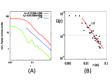
Figure 1: Average vorticity profile observed in simulations (A, Fig. 2C from Chertkov et al. (2007)) and experiment (B, Fig. 3 from Xia et al. (2009)).

Laboratory experiments showed that the coherent flow contains one or two vortices, depending on the boundary conditions, and taking roughly a half of the system size Clercx and van Heijst (2009); Xia et al. (2009). Numerical simulations of Chertkov et al. (2007) reported a well-defined scaling for the average velocity profile in the interior, $V\propto r^{-\eta}$, as a function of distance, $r$, from the vortex center, and $\eta\approx 1/4$. Similar scaling was also observed in the thin layer experiment Xia et al. (2009). Fig. 1 summarizes the results of Chertkov et al. (2007); Xia et al. (2009) for the average vorticity, $\Omega$, demonstrating the $\propto r^{-5/4}$ behavior corresponding to $\eta=1/4$. (We mention the experimental results of Xia et al. (2009) to emphasize emergence of the scaling range, possibly not reached in preceding experiments, e.g. Clercx and van Heijst (2009), presumably because of a somehow higher surface friction. )

Our main result is a rigorous derivation of the $\eta=1/4$ scaling and explanation of why this scaling is universal. Our derivation is the first of the kind in the field of turbulence as predicting universal scaling for a structure emerging as the result of a nonlinear balance between the small-scale turbulence and the coherent structure generated by turbulence. The key feature that allowed us to derive this analytical result, is the smallness of the amplitude of the background velocity fluctuations in comparison with the coherent part. In essence, this small parameter provides an asymptotically accurate truncation of the generally infinite system of Hopf equations on the level of third order correlation functions of velocity/vorticity. The $\eta=1/4$ scaling emerges from an explicit solution of the resulting system of equations. The main contribution to the third-order Hopf equation (for the third order correlation function) is associated with a zero mode of the respective integro-differential operator representing the homogeneous part of the equation. This result is substituted into the second-order Hopf equation, thus treated as a linear inhomogeneous equation for the pair-correlation function, with the third-order correlation function calculated on the previous step. Similarly, the first order Hopf equation is a linear inhomogeneous equation with respect to the first moment (the coherent term), resulting in a closed expression for the scaling exponent. Our strategy below is to derive the set of equations, introduce the truncations and show that a scale-invariant expression with $\eta=1/4$ gives a solution consistent with the assumptions made in the process of the derivations.

The 2D velocity field $\bm{v}$ is assumed controlled by the Navier-Stocks equation

$$\partial_{t}\omega+({\bm{v}}\nabla)\omega=-\alpha\omega+\nu\nabla^{2}\omega+\mathrm{curl}\,{\bm{f}},$$ (1)

formulated in terms of the vorticity $\omega=\mathrm{curl}\,\bm{v}$. One assumes that the fluid is incompressible, $\nabla\cdot{\bm{v}}=0$. The terms on the right-hand side of Eq. (1) represent the bottom friction, the viscosity and the turbulent forcing respectively. The force per unit mass, $\bm{f}$, is assumed to be random, zero mean, statistically homogeneous in space and time, and correlated at an intermediate scale, $l$, called pumping scale. We study the case in which the pumping scale is much smaller than the size of the system (of the box), $L$, and it is much larger than the Kolmogorov (viscous) scale, $r_{\mathrm{visc}}$. The energy density (per unit mass) $\varepsilon$ injected by the forcing ${\bm{f}}$ in a unit of time per unit mass is considered constant in space and time.

If one starts from zero velocity and turns on the pumping ${\bm{f}}$ at $t=0$, in time $\tau_{d}\sim l^{2/3}/\varepsilon^{1/3}$ a direct enstrophy cascade is established in the range of scales between the pumping scale and the viscous scale. The establishment of this direct cascade is followed by a much slower growth of the inverse energy cascade from the pumping scale to larger scales. The energy-containing scale of the inverse cascade grows, as $l_{inv}\sim\varepsilon^{1/2}t^{3/2}$, until the scale reaches the system size $L$ at time $\tau_{inh}\sim(L^{2}/\varepsilon)^{1/3}$. After that the system has no choice but to deviate from spatially homogeneous KLB regime, producing a large-scale coherent flow. This picture is correct provided the bottom friction is sufficiently weak, $\alpha\ll\epsilon^{1/3}L^{-2/3}$, as assumed in the following. Establishing the spatial profile of the resulting average velocity at times $t>\tau_{inh}$ is our main objective.

Once the large-scale coherent flow has emerged, the total velocity field, ${\bm{v}}(t,{\bm{r}})$, can be decomposed into coherent and fluctuating parts, ${\bm{v}}(t,{\bm{r}})={\bm{V}}(t,{\bm{r}})+{\bm{u}}(t,{\bm{r}})$. By definition of the coherent part, $\langle{\bm{u}}\rangle=0$, where angular brackets indicate averaging over the temporal scale of the vortex turnover time, $\sim L/V$. After a transient period, i.e. once the large-scale flow has matured, the injected energy is mainly accumulated in the coherent component of the velocity ${\bm{V}}(t,{\bm{r}})$, which grows slowly in time, $\propto\sqrt{t}$, corresponding to the linear in time growth of the total energy. Ultimately, the average velocity profile $\bm{V}$ is stabilized by the bottom friction, then the velocity amplitude is determined by the balance between energy injection and dissipation, where thus $V\propto 1/\sqrt{\alpha}$. Let us consider averaging Eq. (1)

$$(\partial_{t}+\alpha)\Omega+{\bm{V}}\nabla\Omega+\nabla\langle{\bm{u}}\varpi\rangle=0,$$ (2)

where $\Omega=\langle\omega\rangle$ is the average vorticity and $\varpi=\mathrm{curl}\,\bm{u}$ stands for respective fluctuations. In Eq. (2) we have ignored viscosity and dropped pumping, both irrelevant at scales larger than $l$. Our description, detailed below, is based on the assumption that the coherent flow dominates fluctuations, $V\gg u$, possibly everywhere except for a small neighborhood of the vortex core. (This assumption can be accurately verified via a self-consistent multi-step procedure including an analysis of the multi-point correlation functions. A detailed discussion of these technical details is postponed for a longer publication.)

In the periodic set-up, e.g. realized in simulations Chertkov et al. (2007), a pair of vortexes forming a dipole is formed, whereas in a bounded box set-up one observes a single vortex, as seen in the experiment of Xia et al. (2009). Other structures, e.g. more than one pair of vortices or stripes or combinations of stripes and vortexes, can also emerge in boxes of special shapes, such as those with large aspect ratios or non-trivial topology (e.g., stripes and rings) Chavanis and Sommeria (1996); Yin et al. (2003). In the following we will focus on an analysis of a vortex which applies equally well to either of the two cases mentioned above. (Note also that our approach to describing the shape of the vortex is based on analysis of stochastic Navier-Stokes, and as such it is distinctly different from the quasi-equilibrium 2d approach Robert and Sommeria (1991); Chavanis and Sommeria (1996); Yin et al. (2003), postulating a distribution of Gibbs-kind controlled by the set of lagrangian multipliers associated with different moments of vorticity.)

An emergence of the coherent vortices results in an inhomogeneous redistribution of energy. After a vortex (or pair of vortexes) has emerged, the global profile of ${\bm{V}}(t,\bm{r})$ shows two regions, corresponding to a vortex exterior and an interior respectively. In the vortex exterior the average velocity is estimated as $V\sim\sqrt{\epsilon t}$ or $V\sim\sqrt{\epsilon/\alpha}$ (the latter corresponds to the stationary case, in which the turbulence is stabilized by friction), while inside the vortex the coherent part is much larger and (up to small variations we are ignoring) its components are $V_{\varphi}=V(r)$ and $V_{r}=0$. Inspired by the results of the numerical Chertkov et al. (2007) and laboratory Xia et al. (2009) experiments, we assume that the spatial profile of the coherent part in the interior of the vortex is algebraic, that is

$$V(t,\bm{r})=V_{0}(L/r)^{\eta},$$ (3)

where the distance $r$ is measured from the vortex center and $V_{0}$ estimates the coherent part of the velocity in the vortex exterior. Eq. (3) is correct for the $r_{\mathrm{core}}\ll r\ll L$ range. Here $r_{\mathrm{core}}$ is the size of the vortex core. The term, $\bm{V}\nabla\Omega$, in Eq. (2) is zero due to the isotropy of the vortex. Therefore the vortex profile is determined by a balance of the first and third terms in Eq. (2). Obviously, Eq. (2) is not closed and one naturally needs to consider an additional equation for the pair correlation function of velocity/vorticity fluctuations inside the vortex.

In fact, it is convenient to derive these extra equations for the averages in two steps, first rewriting Eq. (1)

$$(\partial_{t}+\alpha)u_{r}+\partial_{\varphi}\hat{\cal N}^{-1}\hat{\cal K}u_{r}-\partial_{\varphi}r^{2}\hat{\cal N}^{-1}(\bm{u}\nabla\varpi)=0\,,$$ (4)

where both the force and the viscosity terms are dropped. The differential operators in Eq. (4) are

$$\hat{\cal N}=r[(\partial_{\varrho}+1)^{2}+\partial_{\varphi}^{2}]\,,$$ (5)

$$\hat{\cal K}=V(\partial_{\varrho}^{2}+2\partial_{\varrho}+2+\partial_{\varphi}^{2})-(\partial_{\varrho}^{2}V)\,,$$ (6)

where $\varrho=\ln(r/L)$. Then, we introduce the pair correlation function of the radial velocity fluctuations

$$\Phi(t,r_{1},r_{2},\varphi)=\langle u_{r}(t,r_{1},\varphi_{1})u_{r}(t,r_{2},\varphi_{2})\rangle\,,$$ (7)

where $\varphi=\varphi_{1}-\varphi_{2}$. The correlation function is invariant under the transformation, $\varphi\to-\varphi$, $r_{1}\leftrightarrow r_{2}$, corresponding to the permutation of the points labeled by $1$ and $2$. Using this property and assuming analyticity of the pair correlation function (7) for small $\varphi$ and $\rho=\ln(r_{1}/r_{2})$, we derive the following expression for the single-point cross-object of the second-order, $\langle u_{r}\varpi\rangle$, appearing in Eq. (2):

$$\langle u_{r}\varpi\rangle=-\left.\frac{2}{r}\hat{B}\partial_{\rho}\partial_{\varphi}^{-1}\Phi(r,\rho,\varphi)\right|_{\rho=0,\varphi=0}\,,$$ (8)

where $r=\sqrt{r_{1}r_{2}}$ and $\hat{B}=1+r\partial_{r}/2$. Note that only antisymmetric in $\varphi$ term in $\Phi$ contributes to $\langle u_{r}\varpi\rangle$.

Multiplying Eq. (4) by the velocity at another spatial point and averaging the resulting equation over fluctuations, one derives

$$\hat{\cal N}_{1}^{-1}\hat{\cal N}_{2}^{-1}\left(\hat{\cal N}_{2}\hat{\cal K}_{1}-\hat{\cal N}_{1}\hat{\cal K}_{2}\right)\Phi(r_{1},r_{2},\varphi)$$

$$=r_{1}^{2}\hat{\cal N}_{1}^{-1}\nabla_{1}\left\langle\bm{u}(\bm{r}_{1})\varpi(\bm{r}_{1})u_{r}(\bm{r}_{2})\right\rangle$$

$$-r_{2}^{2}\hat{\cal N}_{2}^{-1}\nabla_{2}\left\langle u_{r}(\bm{r}_{1})\bm{u}(\bm{r}_{2})\varpi(\bm{r}_{2})\right\rangle\,,$$ (9)

where the irrelevant (asymptotically small) terms, containing the time derivative and the friction coefficient $\alpha$, are omitted. The operator on the left hand side of Eq. (9) can be rewritten as

$$\hat{\cal N}_{2}\hat{\cal K}_{1}-\hat{\cal N}_{1}\hat{\cal K}_{2}=(r_{2}V_{1}-r_{1}V_{2})\times$$

$$\biggl{\{}[\partial_{\rho}^{2}+\partial_{\varphi}^{2}+\hat{B}^{2}]^{2}+(1-\eta^{2})[\partial_{\rho}^{2}+\partial_{\varphi}^{2}+\hat{B}^{2}]$$

$$-4\hat{B}^{2}\partial_{\varrho}^{2}+2\hat{B}(1-\eta^{2})\coth[(1+\eta)\rho/2]\partial_{\rho}\biggr{\}}.$$ (10)

When the separation $\bm{r}_{1}-\bm{r}_{2}$ is sufficiently small, the right hand side of Eq. (9) controls the inverse energy flux, exactly as in the traditional KLB case. Indeed, in the spatially homogeneous case, the correlation function $\left\langle u_{\alpha}(\bm{r}_{1})\varpi(\bm{r}_{1})u_{\beta}(\bm{r}_{2})\right\rangle\sim\epsilon$ depends solely on $\bm{r}_{1}-\bm{r}_{2}$ and it is also divergentless due to $\nabla\bm{u}=0$. Substituting the Kolmogorov estimate $\Phi-\Phi(0)\sim(\epsilon|\bm{r}_{1}-\bm{r}_{2}|)^{2/3}$ into the left hand side of Eq. (9), one finds that the term is negligible for $|\bm{r}_{1}-\bm{r}_{2}|=r_{12}\ll\zeta_{\star}$, where $\zeta_{\star}(r)=\alpha^{3/4}r^{3/2}\epsilon^{-1/4}(r/L)^{3\eta/2}$ is thus an important scale dependent on the distance from the vortex core, $r$. One concludes that for $r_{12}\gg\zeta_{\star}(r)$, the inverse cascade is modified by the coherent flow.

However, due to isotropy the term in $\Phi$ related to the KLB cascade does not contribute to the object of our prime attention, $\langle{\bm{u}}\varpi\rangle$. First, we look for such solutions, also remaining regular at small $r_{12}$, in terms of the zero modes of the operator on the left-hand side of Eq. (9), thus ignoring the smaller right-hand side in the equation. However, these zero modes do not contribute to $\langle u_{r}\varpi\rangle$, because the last term in the operator (10) prohibits odd in $\rho$ zero modes to be regular for small $\rho$. Therefore, to extract a non-zero contribution to $\langle u_{r}\varpi\rangle$, one has to account for a correction to $\Phi$, $\delta\Phi$, related to the right-hand side of Eq. (9). To get a non-trivial contribution one ought to carry our analysis to the next order in the Hopf hierarchy describing the triple velocity correlation function, $F=\langle v_{r}(\bm{r}_{1})v_{r}(\bm{r}_{2})v_{r}(\bm{r}_{3})\rangle$.

The principal terms in the third-order Hopf equation governing $F$ are

$$\left\{\frac{\partial}{\partial\varphi_{1}}\hat{\cal N}_{1}^{-1}\hat{\cal K}_{1}\!+\!\frac{\partial}{\partial\varphi_{2}}\hat{\cal N}_{2}^{-1}\hat{\cal K}_{2}\!+\!\frac{\partial}{\partial\varphi_{3}}\hat{\cal N}_{3}^{-1}\hat{\cal K}_{3}\right\}F=0.$$ (11)

where we again omitted asymptotically irrelevant terms, including the time derivative term, the friction term and also the contribution related to the fourth order correlation function. Formally, any zero mode of the operator $K$ satisfies Eq. (11), and the quest is to find the scale-invariant zero mode of $K$, $Z_{m}=\exp(im\varphi+\beta_{m}\varrho)$ where $m$ is an integer (to guarantee smoothness at the smallest scales) and $\beta_{m}=\sqrt{m^{2}+\eta^{2}-1}-1$, which generates a nonzero contribution into $\langle u_{r}\varpi\rangle$ via Eqs. (9,8) and has the smallest possible $\beta_{m}$. The first terms in the hierarchy of possible candidates are

$$F\propto Z_{m}(r_{1},\varphi_{1})Z_{k}(r_{2},\varphi_{2})Z_{-m-k}(r_{3},\varphi_{3})+\dots,$$ (12)

where the dots represent the sum of the terms that are obtained from the first product in Eq. (12) by permuting the indices $1,2,3$. However, the expression (12) generates an odd outcome for the right-hand side of Eq. (9), thus resulting in an even correction $\delta\Phi$ giving no contribution to $\langle u_{r}\varpi\rangle$. Therefore, one has to look for higher order terms in the hierarchy. One finds that the desired zero mode can can be constructed with the help of an auxiliary object, $X_{m}=\exp[im\varphi+(\beta_{m}+1+\eta)\varrho]$, satisfying $(\hat{\cal N}_{m})^{-1}\hat{\cal K}_{m}X_{m}=A_{m}Z_{m}$, where $A_{m}$ are real numbers:

$$F=\alpha_{m}X_{m}(r_{1},\varphi_{1})Z_{k}(r_{2},\varphi_{2})Z_{-m-k}(r_{3},\varphi_{3})+\dots$$

$$+\alpha_{k}Z_{m}(r_{1},\varphi_{1})X_{k}(r_{2},\varphi_{2})Z_{-m-k}(r_{3},\varphi_{3})+\dots$$

$$+\alpha_{-k-m}Z_{m}(r_{1},\varphi_{1})Z_{k}(r_{2},\varphi_{2})X_{-m-k}(r_{3},\varphi_{3})+\dots,$$ (13)

and the dots stand for the sum of terms which accounts for respective permutations. Eq. (13) is a solution of Eq. (11), provided $\alpha_{m}mA_{m}+\alpha_{k}kA_{k}-\alpha_{-m-k}(m+k)A_{-m-k}=0$. Choosing $m=k=1$ we find a term giving a non-odd $\propto r^{3\eta+\sqrt{3+\eta^{2}}-3}$ contribution to the right hand side of Eq. (9). Then the correction to the pair correlation function is $\delta\Phi\propto r^{4\eta+\sqrt{3+\eta^{2}}-2}$. This result, finally substituted into the last term in Eq. (2), translates into the $4\eta-3+\sqrt{3+\eta^{2}}=-\eta$ relation, whose solution is $\eta=1/4$. To conclude, the $ZZZ$ and $ZZX$ terms, represented by Eqs. (12) and Eqs. (13), are the only structures possibly contributing to the third-order correlation function $F$, and of the various allowed (nonzero) contributions, the $ZZX$ term (13) with $m=k=1$ dominates $F$ at $r_{1,2}\ll L$.

Substituting the expressions, corresponding to $\eta=1/4$, into the the Hopf equations of the first, second and third orders and estimating all the terms dropped in the derivation process confirms the validity of our asymptotic approximations. This completes our derivations.

We now summarize our results. The main and somewhat surprising result we just derived conserns universality of the vortex mean profile. The scaling of the vortex shape is controlled primarily by a nontrivial zero mode of the operator on the right-hand side of Eq. (11) and otherwise it follows from scaling relations between pairs of terms in the first- and second-order Hopf equations. Nothing in this solution is sensitive to the geometry of the box, or the details of the pumping. The solution also does not depend on the type of viscosity (hyper or normal), or the damping coefficient. Our conclusion does not depend of whether or not the coherent part grows in time or if it was already saturated by damping. Finally, our results make predictions going far beyond the main scaling statement, in particular detailed structure of angular harmonics is predicted for pair and triple correlation functions in the coherent regimes. Our theoretical statements call for accurate experimental and numerical tests.

We conclude by mentioning a number of other comprehensive questions raised by this study. Suppose a vortex or a pair of vortexes, internally tuned and built up from the energy flux are produced, but then the pumping is switched off. Will the initially formed vortex will keep its shape dynamically? Also if a somewhat different in shape, non-universal and large scale vortex is created, will it transform via decaying turbulence into the universal shape predicted above? We conjecture that answers to both the questions are affirmative. These questions certainly require careful investigation in the future.

The work at LANL was carried out under the auspices of the National Nuclear Security Administration of the U.S. Department of Energy at Los Alamos National Laboratory under Contract No. DE-AC52-06NA25396. The work of I.K. and V.L. was partially supported by RFBR under grant no. 09-02-01346-a and FTP “Kadry”.

References

- Kraichnan (1967) R. H. Kraichnan, Phys. of Fluids 10, 1417 (1967).
- Leith (1968) C. E. Leith, Physics of Fluids 11, 671 (1968).
- Batchelor (1969) G. K. Batchelor, Physics of Fluids 12, II (1969).
- Smith and Yakhot (1994) L. M. Smith and V. Yakhot, JFM 274, 115 (1994).
- Borue (1994) V. Borue, PRL 72, 1475 (1994).
- Jin and Dubin (2000) D. Z. Jin and D. H. E. Dubin, PRL 84, 1443 (2000).
- Shats et al. (2005) M. G. Shats, H. Xia, and H. Punzmann, PRE 71, 046409 (2005).
- Xia et al. (2008) H. Xia, H. Punzmann, G. Falkovich, and M. G. Shats, PRL 101, 194504 (2008).
- Xia et al. (2009) H. Xia, M. Shats, and G. Falkovich, Phys.Fluids 21, 125101 (2009).
- Chertkov et al. (2007) M. Chertkov, C. Connaughton, I. Kolokolov, and V. Lebedev, PRL 99, 084501 (2007).
- Lesieur (1997) M. Lesieur, Turbulence in Fluids (Kluwer, 1997).
- Charney (1971) J. D. Charney, J. Atmos. Sci. 28 (1971).
- Nastrom and Gage (1985) G. D. Nastrom and K. S. Gage, J. Atmos. Sci. 42 (1985).
- Frisch (1995) U. Frisch, Turbulence: The Legacy of A. N. Kolmogorov (Cambridge University Press, 1995).
- Boffetta et al. (2000) G. Boffetta, A. Celani, and M. Vergassola, PRE 61 (2000).
- Paret and Tabeling (1998) J. Paret and P. Tabeling, Physics of Fluids 10, 3126 (1998).
- Kellay and Goldburg (2002) H. Kellay and W. I. Goldburg, Reports on Progress in Physics 65, 845 (2002).
- Chen et al. (2006) S.-Y. Chen, R. E. Ecke, G. L. Eyink, M. Rivera, M. Wan, and Z. Xiao, PRL 96, 084502 (2006).
- Rutgers (1998) M. A. Rutgers, PRL 81, 2244 (1998).
- Smith and Yakhot (1993) L. M. Smith and V. Yakhot, PRL 71, 352 (1993).
- Clercx and van Heijst (2009) H. J. H. Clercx and G. J. F. van Heijst, Applied Mech. Rev. 62, 020802 (pages 25) (2009).
- Chavanis and Sommeria (1996) P. H. Chavanis and J. Sommeria, JFM 314, 267 (1996).
- Yin et al. (2003) Z. Yin, D. C. Montgomery, and H. J. H. Clercx, Phys. of Fluids 15, 1937 (2003).
- Robert and Sommeria (1991) R. Robert and J. Sommeria, JFM 229, 291 (1991).