The dangers of deprojection of proper motions

Abstract

We re-examine the method of deprojection of proper motions, which has been used for finding the velocity ellipsoid of stars in the nearby Galaxy. This method is only legitimate if the lines of sight to the individual stars are uncorrelated with the stars’ velocities. Very simple models are used to show that spurious results similar to ones recently reported are obtained when velocity dispersion decreases with galactocentric radius in the expected way. A scheme that compensates for this bias is proposed.

1 Introduction

Dehnen & Binney (1998, hereafter DB98) introduced a method for deprojecting proper-motion data, which allowed them to explore the velocity distribution of nearby stars in the Hipparcos catalogue (ESA, 1997), without knowing their radial velocities. This works by taking a weighted ensemble average of the proper motions of stars found in different parts of the sky, under the assumption that the velocity distribution is uncorrelated with position on the sky. This assumption was legitimate in the case of the sample studied by DB98 because all its stars lay within $\sim 100\,\mathrm{pc}$ of the Sun, so it was reasonable to approximate the full phase space distribution function by the velocity-space distribution at the Sun: $f(\mathbf{x},\mathbf{v})\simeq f(\mathbf{x}_{\odot},\mathbf{v})$.

Recently Fuchs et al. (2009, hereafter F09) used the DB98 technique to study a sample of stars taken from the Sloan Digital Sky Survey (SDSS: Abazajian et al., 2009). This data set contains stars that extend up to $\sim 800\,\mathrm{pc}$ above the plane and span a range of galactocentric radii $\sim 2\,\mathrm{kpc}$ wide. Since the velocity dispersion of stars varies with both radius and distance from the plane, the validity of the assumption that the velocity distribution is uncorrelated with sky position is questionable for this spatially extended sample. In this paper we demonstrate that applying the DB98 technique leads to erroneous results, particularly with regard to the tilt of the velocity ellipsoid with respect to the Galactic plane.

In Section 2 we briefly explain the DB98 method, and in Section 3 we demonstrate that for a sample like that of F09 it gives a biased estimate of the tilt of the velocity ellipsoid. Section 3.1 explains the origin of this bias physically. Section 3.2 proposes a technique for removing the bias. In Section 4 we discuss biases in the DB98 technique more generally.

2 Deprojection

The deprojection equations are stated and explained by DB98, and written out in full by F09. We repeat them here for clarity.

We work in a Cartesian coordinate system, centred on the Sun, in which the $x$-axis points towards the Galactic centre, the $y$-axis points in the direction of Galactic rotation, and the $z$-axis points towards the north Galactic pole. Given a star moving with heliocentric velocity $\mathbf{v}\equiv(U,V,W)$, the observed proper-motion velocity is

$$\mathbf{p}=\mathbf{v}-v_{\parallel}\mathbf{\hat{s}},$$ (1)

where $\mathbf{\hat{s}}$ is the unit vector pointing from the Sun to the star, and $v_{\parallel}$ is the component of $\mathbf{v}$ parallel to $\mathbf{\hat{s}}$. This can be written in matrix form as

$$\mathbf{p}=\mbox{\boldmath{$\mathsf{A}$}}\cdot\mathbf{v},\quad\mbox{where}\quad A_{ij}=\delta_{ij}-\hat{s}_{i}\hat{s}_{j}.$$ (2)

The velocity ellipsoid is defined by both the mean velocity and the velocity dispersion. To determine the velocity dispersion tensor we use the equation

$$p_{i}p_{j} = \sum_{k,l}A_{ik}v_{k}\,A_{jl}v_{l}$$ (3)

$$= \sum_{kl}B_{ijkl}v_{k}v_{l},$$

where

$$B_{ijkl}\equiv\frac{1}{2}(A_{ik}\,A_{jl}+A_{il}\,A_{jk})$$ (4)

is the part of $\mathsf{A}$$\mathsf{A}$ that is symmetric in its last pair of indices.

We are interested in situations in which we know $\mathbf{p}$ and $\mathbf{\hat{s}}$ (and therefore $\mathsf{A}$ and $\mathsf{B}$) but do not know $\mathbf{v}$. It is clear from the definition of $\mathbf{p}$ (equation 1) that in this case we cannot find $\mathbf{v}$ for an individual star because we do not know $v_{\parallel}$. This is reflected in the fact that $\mathsf{A}$ is singular.

We average equations (2) and (3) over a sample of stars. If the velocities $\mathbf{v}$ of these stars are uncorrelated with their sky positions $\mathbf{\hat{s}}$, they will be uncorrelated with $\mathsf{A}$ and $\mathsf{B}$, and the expectation value of a product such as $\mbox{\boldmath{$\mathsf{A}$}}\cdot\mathbf{v}$ will equal the expectation of $\mathsf{A}$ times the expectation of $\mathbf{v}$. That is, when the velocities are not correlated with $\mathbf{\hat{s}}$

$$\langle\mathbf{p}\rangle=\langle\mbox{\boldmath{$\mathsf{A}$}}\cdot\mathbf{v}\rangle=\langle\mbox{\boldmath{$\mathsf{A}$}}\rangle\cdot\langle\mathbf{v}\rangle.$$ (5)

Provided the stars are sufficiently widely spread on the sky, the matrix $\langle\mbox{\boldmath{$\mathsf{A}$}}\rangle$ is not singular, so we can write

$$\langle\mathbf{v}\rangle=\langle\mbox{\boldmath{$\mathsf{A}$}}\rangle^{-1}\cdot\langle\mathbf{p}\rangle.$$ (6)

Similarly,

$$\langle\mathbf{vv}\rangle=\langle\mbox{\boldmath{$\mathsf{B}$}}\rangle^{-1}\cdot\langle\mathbf{pp}\rangle.$$ (7)

3 Tests

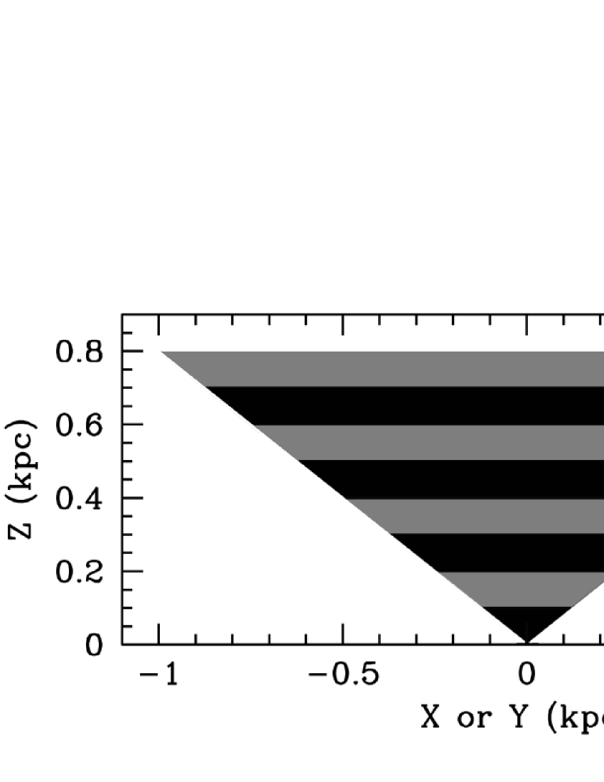
Figure 1: Position of the 8 counting volumes, shaded black or grey alternately as we look further from the plane, that make up a cone with its vertex at the Sun, and its axis perpendicular to the Galactic plane.

In this section we demonstrate the danger of using the DB98 technique when the key assumption of uncorrelated $\mathbf{v}$ and $\mathbf{\hat{s}}$ does not hold. We do this by considering a simplified form of the problem addressed by F09, which was to find the velocity ellipsoid of stars in the SDSS survey volume. Fig. 1 shows our idealisation of the F09 counting volumes – we take them to be slices of a cone with the Sun as its apex. In our usual Cartesian coordinate system centred on the Sun, the cone is defined by $\sqrt{X^{2}+Y^{2}}<0.8Z$ and $Z<800\,\mathrm{pc}$. It is split into eight counting volumes that are each $100\,\mathrm{pc}$ thick (cf Fig. 5 of F09).

F09 validated their use of the DB98 method by drawing a velocity for every star in their sample from a Schwarzschild distribution with a velocity ellipsoid that was everywhere aligned with the $X,Y$ and $Z$ axes, and had constant axis lengths $\sigma_{U}$, $\sigma_{V}$ and $\sigma_{W}$. This velocity distribution does not vary with position, so $\mathbf{v}$ and $\mathbf{\hat{s}}$ will be uncorrelated. In reality the velocity ellipsoid will vary from point to point, both in the orientation of its principal axes, and in the lengths of these axes. The lengths of these axes are expected to vary with galactocentric radius $R$ roughly as $\mbox{\boldmath$\sigma$}\propto\exp(-R/R_{\sigma})$, where $R_{\sigma}$ is of order twice the disc’s scale length $R_{\rm d}$ (e.g. Binney & Tremaine, 2008). In the Milky Way, $R_{\rm d}\simeq 2.5\,\mathrm{kpc}$ (e.g. Jurić et al., 2008), so $R_{\sigma}\sim 5\,\mathrm{kpc}$.

To illustrate the difficulty we adopt the distribution function

$$f \propto \exp\left\{-\frac{1}{2}\left[\left(\frac{v_{R}}{\sigma_{R}(R,z)}\right)^{2}\right.\right.+$$ (9)

$$\left.\left.\left(\frac{v_{\phi}-v_{c}(R)-\langle v_{\phi}(R,z)\rangle}{\sigma_{\phi}(R,z)}\right)^{2}+\left(\frac{v_{z}}{\sigma_{z}(R,z)}\right)^{2}\right]\right\}.$$

where again $(R,\phi,z)$ are cylindrical coordinates centred on the Galactic Centre, $v_{c}(R)$ is the circular speed, and $\langle v_{\phi}(R,z)\rangle$ is the asymmetric drift. The velocity ellipsoid for this distribution function is aligned with the cylindrical coordinate axes. We assume that we can correctly compensate for the circular velocity using Oort’s constants (e.g. Feast & Whitelock, 1997). In all cases we take constant $\langle v_{\phi}(R,z)\rangle=-26\,\mathrm{km\,s}^{-1}$. In practice $\langle v_{\phi}\rangle$ varies with $\sigma$, but this makes virtually no difference to these results, so we ignore it for simplicity.

We consider the following three forms for $\sigma$:

1. Constant $\mbox{\boldmath$\sigma$}\equiv(\sigma_{R},\sigma_{\phi},\sigma_{z})=(45,32,24)\,\mathrm{km\,s}^{-1}$. This is nearly the same distribution function used by F09, except with the velocity ellipsoid aligned with the cylindrical rather than Cartesian axes.

2. Radially varying $\sigma$

   $$\mbox{\boldmath$\sigma$}(R)=\mbox{\boldmath$\sigma$}(R_{0})\,\exp[(R_{0}-R)/R_{\sigma}]$$ (10)

   with $R_{\sigma}=5\,\mathrm{kpc}$, $R_{0}=8\,\mathrm{kpc}$, and $\mbox{\boldmath$\sigma$}(R_{0})$ taking the same value as in case 1.

3. A form that varies both radially and vertically so as to provide reasonable fits to the dispersions reported by F09:

   $$\mbox{\boldmath$\sigma$}(R,z)=(34+20z,23 + 20z,19+30z)\,\mathrm{km\,s}^{-1}$$ (11)

   $$\times \exp[(R_{0}-R)/R_{\sigma}],$$

   where $R_{\sigma}=5\,\mathrm{kpc}$ and $z$ is expressed in $\mathrm{kpc}$.

In each counting volume, we place 100,000 stars drawn randomly from a uniform probability distribution over the entire volume. We assign each star a velocity randomly chosen from the distribution function. We then “observe” this star, and find its proper motion. This allows us to compare the values of $\mathbf{v}$ and $\mathbf{v}\mathbf{v}$ we determine from deprojection (equations 6 & 7) to the real values.

Since we consider everything with respect to the Cartesian axes defined in Section 2, this yields values for $\langle U\rangle$, $\langle UU\rangle$, $\langle UV\rangle$, etc. We can use these values (and the fact that the centre of each counting volume lies at $X=Y=0$) to find the velocity dispersions parallel to the cylindrical axes, $\sigma_{R},\,\sigma_{\phi}$ and $\sigma_{z}$ and the mixed moments $\sigma_{R\phi}^{2},\,\sigma_{Rz}^{2}$ and $\sigma_{\phi z}^{2}$.

Note that the mixed moments may be either positive or negative. In Figs. 2, 3 & 4 we plot $\sigma_{R\phi}$, $\sigma_{Rz}$ and $\sigma_{\phi z}$, which we define by

$$\sigma_{ij}\equiv\mathrm{sign}(\sigma^{2}_{ij})\sqrt{|\sigma^{2}_{ij}|}.$$ (12)

The two vertex deviations, which describe the orientation of the velocity ellipsoid with respect to the cylindrical axes, can be found from these values as

$$\Psi=-\frac{1}{2}\arctan{\frac{2\sigma^{2}_{R\phi}}{\sigma^{2}_{R}-\sigma^{2}_{\phi}}};$$ (13)

$$\alpha=-\frac{1}{2}\arctan{\frac{2\sigma^{2}_{Rz}}{\sigma^{2}_{R}-\sigma^{2}_{z}}}.$$ (14)

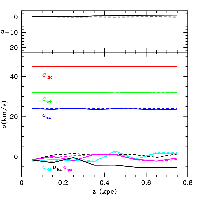
Figure 2: Components of the velocity dispersion tensor $\sigma$ (bottom) and the velocity ellipsoid tilt angle with respect to the plane, $\alpha$ (top) as a function of height above the plane. The figure shows the true values from the sample in each counting volume (dotted) and the values found by deprojection (solid). The true velocity ellipsoid has principal axes aligned with the cylindrical coordinate directions and axis lengths that are independent of position (i.e. $\mbox{\boldmath$\sigma$}=\mathrm{const}$).

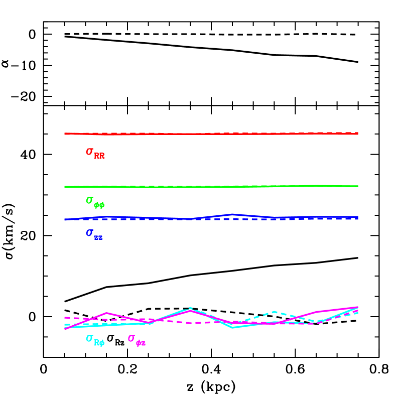
Figure 3: Similar to Fig. 2, except for $\mbox{\boldmath$\sigma$}\propto\exp(-R/R_{\sigma})$, with $R_{\sigma}=5\,\mathrm{kpc}$. Again, dotted lines show the true values, and solid lines show those found by deprojection.

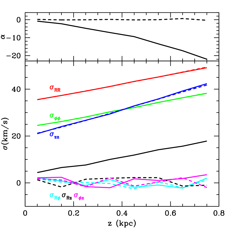
Figure 4: Similar to Figs. 2 and 3, with $\mbox{\boldmath$\sigma$}\propto\exp(-R/R_{\sigma})$, with $R_{\sigma}=5\,\mathrm{kpc}$, and with $\sigma$ varying with $z$ (as can be seen in the figure). Again, dotted lines show the true values, and solid lines show those found by deprojection. The value of $\sigma_{Rz}$ found here is similar to that found in Figure 3, with the angle $\alpha$ being larger at large $z$ because the velocity ellipsoid is rounder, due to $\sigma_{z}$ increasing more than $\sigma_{R}$ (c.f. equation 14).

In each of these cases, the values of $\langle U\rangle$, $\langle V\rangle$ and $\langle W\rangle$ determined from equation (6) are consistent with the true values at $R_{0}$.

The lower panels of Figs. 2, 3 & 4 show the values of these velocity dispersions and the mixed moments as functions of distance from the plane for the three distribution functions described above: true values are shown by dotted lines, while solid lines show values recovered by deprojection. We see that deprojection yields reasonably accurate values of $\sigma_{R}$, $\sigma_{\phi}$, $\sigma_{z}$, $\sigma_{R\phi}$ and $\sigma_{\phi z}$ even when $\sigma$ varies significantly through the counting volumes, so the DB98 procedure is not strictly valid.

However, the value of $\sigma_{Rz}$ found by deprojection is materially incorrect in all cases, being slightly negative when $\sigma$ does not vary with $R$, and positive otherwise. The upper panels of Figs. 2, 3 & 4 show that these incorrect values of $\sigma_{Rz}$ yield values of the tilt angle as large as $\alpha\simeq-20\degr$. A tilt of the long axis of the ellipsoid towards the plane implied by $\alpha\simeq-20\degr$ is similar to that seen by F09. Thus our experiments demonstrate that the F09 tilt could be an artifact that arises because the velocity dispersion increases inwards.

3.1 Physical interpretation

To understand why a radial gradient in $\sigma$ leads to an apparent tilt of the velocity ellipsoid towards the plane, consider a simplified case in which there are two fields, both at Galactic coordinate $b=90-\theta$. One is at $l=0$ and the other is at $l=180$. The velocity measured by the proper motion, $v_{\mu}$, is then

$$v_{\mu}=\left\{\begin{array}[]{ll}v_{R}\cos\theta+v_{z}\sin\theta,&\mbox{ at }l=0;\\ v_{R}\cos\theta-v_{z}\sin\theta,&\mbox{ at }l=180.\\ \end{array}\right.$$ (15)

Since $0<\theta<90$, both $\sin\theta$ and $\cos\theta$ are positive. Therefore, in the field at $l=0$, $v_{\mu}$ is large when $v_{R}$ and $v_{z}$ have the same sign, while in the field at $l=180$ it is large when they take opposite signs. In the absence of a radial gradient, the signature of a tilt towards the plane is therefore larger values of $v_{\mu}$ at $l=0$ than at $l=180$. Clearly a radial gradient in $\sigma$ mimics this signature in the absence of a tilt. Hence if one deprojects under the assumption that there is no radial gradient, the algorithm will account for the data by reporting a tilt towards the plane.

3.2 A workaround

Given that good sky coverage is essential to the success of the DB09 method, one simply cannot assume that the velocity distribution is the same at the locations of all the stars in a sample that reaches out to $\ga 1\,\mathrm{kpc}$ from the Sun. A remedy that can be considered is to adopt a functional form for the radial variation of $\sigma$ and to use this form to correct the observed proper-motion velocities to the values they would have had if $\sigma$ had been independent of position. For example, for each star we could calculate a “corrected” proper-motion velocity

$$\mathbf{p}^{\prime}=(\mathbf{p}-\mbox{\boldmath{$\mathsf{A}$}}\cdot\mathbf{v}_{\mathrm{corr}})\exp[(R-R_{0})/R_{\sigma}^{\prime}]$$ (16)

with $R_{\sigma}^{\prime}$ an estimate for the true value of the parameter $R_{\sigma}$ that controls the radial variation of $\sigma$ (eq. 10) and $\mathbf{v}_{\mathrm{corr}}=\mathbf{v_{\odot}}+\langle v_{\phi}\rangle\mathbf{e}_{\phi}$ an adjustment for the Solar motion and asymmetric drift. Thus defined, $\mathbf{p}^{\prime}$ would be expected to average to zero over all directions and to be the proper-motion velocity if there were no variation in $\sigma$ with radius.

Figure 5: Tilt angle with respect to the Galactic plane ($\alpha$) as a function of height above the plane $z$. The true velocity ellipsoid is oriented parallel to the cylindrical axes, with $\mbox{\boldmath$\sigma$}\propto\exp(-R/(5\,\mathrm{kpc}))$. The figure shows the true value of $\alpha$ for the sample (dotted), the value found from the proper motions without applying any correction (solid), and values found applying a correction (equation 16) with $R_{\sigma}^{\prime}=4\,\mathrm{kpc}$ (short dashed), $5\,\mathrm{kpc}$ (long dashed) and $6\,\mathrm{kpc}$ (dot dashed). The “true” correction, $R_{\sigma}^{\prime}=5\,\mathrm{kpc}$ does not return the true value of $\alpha$ because it does not correct for the fact that the velocity ellipsoid is not aligned with the Cartesian axes.

We test this correction by applying it to simulated data generated as in case (ii) above. We know the true value of $\mathbf{v}_{\mathrm{corr}}$ in this case, so we ignore the relatively minor uncertainties which are caused by not estimating this correctly.

The dashed lines in Fig. 5 show the tilt angle $\alpha$ found from corrected proper-motion velocities for three values of $R_{\sigma}^{\prime}$: $4\,\mathrm{kpc}$ (short-dashed), $5\,\mathrm{kpc}$ (long-dashed) and $6\,\mathrm{kpc}$ (dot-dashed). In all three cases the corrected data give much more accurate results than the uncorrected data (full curve), but the most accurate results are obtained with $R_{\sigma}^{\prime}=6\,\mathrm{kpc}$ rather than the true value, $5\,\mathrm{kpc}$; with $R_{\sigma}^{\prime}=5\,\mathrm{kpc}$ we find $\alpha\sim 1\degr$ at the largest values of $z$ because the correction does not address the problem that the axes of the velocity ellipsoid are aligned with the cylindrical rather than Cartesian axes. A closely related bias is seen when $\sigma$ is constant (Fig. 2). Using a value of $R_{\sigma}^{\prime}=6\,\mathrm{kpc}$ for the correction gives $\alpha\simeq 0$ because it under-compensates for the bias due to the variation in $\sigma$, which inadvertently compensates for the bias due to the alignment of the velocity ellipsoid’s axes.

If we considered the value $\alpha$ well established, we could use corrected proper-motion velocities to determine $R_{\sigma}$ from the data.

4 Discussion

In this paper we have focused on the tilt of the velocity ellipsoid towards the plane, and may have left the reader with the impression that, for example, the tilt in the plane or the non-mixed terms ($\sigma_{R}$ etc.) are correctly recovered by the DB98 technique. While this is true to a good approximation in the cases shown here, it is not always true.

For example, consider the situation described in Section 3.2, in which we need to know the value of $R_{\sigma}$ so we can compensate for the variation in $\sigma$ across the counting volume. In an approach to the determination of $R_{\sigma}$ we might split the data into two sets, for $|l|<90\deg$ and $|l>90\deg$, and find $\sigma$ separately for each set – this gives us enough information to find $R_{\sigma}$. However, if the data are split in this way, they produce a bias in the values of the non-mixed components of $\sigma$ (as well as the mixed components). This bias is in opposite directions for the two data sets, so strongly affects the derived value of $R_{\sigma}$, but cancels out when the two sets are considered together (hence the lack of bias in the non-mixed components in Figs. 3 and 4).

Similar biases must always be considered when using deprojection. In the tests described above, the symmetry of the counting volumes cancelled out the bias in most components of $\sigma$, effectively restricting it to $\sigma_{Rz}$. The counting volumes of real data sets will not enjoy the high degree of symmetry characteristic of our model sets, with the result that biases in the values returned by the DB98 method will not be confined to $\sigma_{Rz}$.

5 Conclusions

In this paper we have demonstrated that the statistical deprojection of proper motions cannot be applied straightforwardly to data spanning a significant volume of the Galaxy. This is primarily because the dependence of the velocity dispersion $\sigma$ on position violates the central assumption of the method.

Using a simple model we have demonstrated that applying this method can suggest a large tilt of the velocity ellipsoid towards the plane, even if the actual tilt is zero. It seems very likely that this effect is responsible for the remarkably large tilt, $\alpha=-20\degr$, reported by F09. Correcting for this effect in the manner discussed in Section 3.2 would probably bring this result much closer to the smaller tilt angles obtained using radial velocities (e.g. Siebert et al., 2008; Bond et al., 2009).

We note, however, that all components of $\sigma$ other than $\sigma_{Rz}$ were nearly unaffected by this bias in our tests. For a realistic survey volume such as that used by F09, these biases are likely to be larger than in our tests and in some circumstances may materially affect the results.

References

- Abazajian et al. (2009) Abazajian K. N., Adelman-McCarthy J. K., Agüeros M. A. et al., 2009, ApJS, 182, 543
- Binney & Tremaine (2008) Binney J., Tremaine S., 2008, Galactic Dynamics: Second Edition. Princeton University Press
- Bond et al. (2009) Bond N. A., Ivezic Z., Sesar B. et al., 2009, ApJ, submitted (arXiv:0909.0013)
- Dehnen & Binney (1998) Dehnen W., Binney J. J., 1998, MNRAS, 298, 387 (DB98)
- ESA (1997) ESA, 1997, VizieR Online Data Catalog, 1239, 0
- Feast & Whitelock (1997) Feast M., Whitelock P., 1997, MNRAS, 291, 683
- Fuchs et al. (2009) Fuchs B., Dettbarn C., Rix H.-W. et al., 2009, AJ, 137, 4149 (F09)
- Jurić et al. (2008) Jurić M., Ivezić Ž., Brooks A. et al., 2008, ApJ, 673, 864
- Siebert et al. (2008) Siebert A., Bienaymé O., Binney J. et al., 2008, MNRAS, 391, 793