Counting colored planar maps: algebraicity results

Abstract.

We address the enumeration of properly $q$-colored planar maps, or more precisely, the enumeration of rooted planar maps $M$ weighted by their chromatic polynomial $\chi_{M}(q)$ and counted by the number of vertices and faces. We prove that the associated generating function is algebraic when $q\not=0,4$ is of the form $2+2\cos(j\pi/m)$, for integers $j$ and $m$. This includes the two integer values $q=2$ and $q=3$. We extend this to planar maps weighted by their Potts polynomial $\operatorname{P}_{M}(q,\nu)$, which counts all $q$-colorings (proper or not) by the number of monochromatic edges. We then prove similar results for planar triangulations, thus generalizing some results of Tutte which dealt with their proper $q$-colorings. In statistical physics terms, the problem we study consists in solving the Potts model on random planar lattices. From a technical viewpoint, this means solving non-linear equations with two “catalytic” variables. To our knowledge, this is the first time such equations are being solved since Tutte’s remarkable solution of properly $q$-colored triangulations.

1. Introduction

In 1973, Tutte began his enumerative study of colored triangulations by publishing the following functional equation [52, Eq. (13)]:

$$T(x,y)=xy^{2}q(q-1)+\frac{xz}{yq}T(1,y)T(x,y)+xz\frac{T(x,y)-y^{2}T_{2}(x)}{y}-x^{2}yz\frac{T(x,y)-T(1,y)}{x-1},$$ (1)

where $T_{2}(x)$ stands for $\frac{1}{2}\frac{\partial^{2}T}{\partial y^{2}}(x,0)$ (in other words, $T_{2}(x)$ is the coefficient of $y^{2}$ in $T(x,y)$). This equation defines a unique formal power series in $z$, denoted $T(x,y)$, which has polynomial coefficients in $q$, $x$ and $y$. Tutte’s interest in this series relied on the fact that it “contains” the generating function of properly $q$-colored triangulations of the sphere (Figure 1). More precisely, the coefficient of $y^{2}$ in $T(1,y)$ is

$$T_{2}(1)=[y^{2}]T(1,y)=q(q-1)+\sum_{T}z^{\operatorname{f}(T)}{\chi_{T}(q)},$$

where the sum runs over all rooted triangulations of the sphere, $\chi_{T}$ is the chromatic polynomial of $T$, and $\operatorname{f}(T)$ the number of faces of $T$.

\begin{picture}(4690.0,2991.0)(3073.0,-2343.0)\end{picture}

Figure 1. A (rooted) triangulation of the sphere, properly colored with 4 colors.

In the ten years that followed, Tutte devoted at least nine papers to the study of this equation [52, 50, 49, 51, 53, 54, 55, 56, 57]. His work culminated in 1982, when he proved that the series $T_{2}(1)$ counting $q$-colored triangulations satisfies a non-linear differential equation [56, 57]. More precisely, with $t=z^{2}$ and $H\equiv H(t)=t^{2}T_{2}(1)$,

$$2q^{2}(1-q)t+(qt+10H-6tH^{\prime})H^{\prime\prime}+q(4-q)(20H-18tH^{\prime}+9t^{2}H^{\prime\prime})=0.$$ (2)

This tour de force has remained isolated since then, and it is our objective to reach a better understanding of Tutte’s rather formidable approach, and to apply it to other problems in the enumeration of colored planar maps. We recall here that a planar map is a connected planar graph properly embedded in the sphere. More definitions will be given later.

We focus in this paper on two main families of maps: general planar maps, and planar triangulations. We generalize Tutte’s problem by counting all colorings of these maps (proper and non-proper), assigning a weight $\nu$ to every monochromatic edge. Thus a typical series we consider is

$$\sum_{M}t^{\operatorname{e}(M)}w^{\operatorname{v}(M)}z^{\operatorname{f}(M)}{\operatorname{P}_{M}(q,\nu)},$$ (3)

where $M$ runs over a given set of planar maps (general maps or triangulations, for instance), $\operatorname{e}(M)$, $\operatorname{v}(M)$, $\operatorname{f}(M)$ respectively denote the number of edges, vertices and faces of $M$, and

$$\operatorname{P}_{M}(q,\nu)=\sum_{c:V(M)\rightarrow\{1,\ldots,q\}}\nu^{m(c)}$$

counts all colorings of the vertices of $M$ in $q$ colors, weighted by the number $m(c)$ of monochromatic edges. As explained in Section 3, $\operatorname{P}_{M}(q,\nu)$ is actually a polynomial in $q$ and $\nu$ called, in statistical physics, the partition function of the Potts model on $M$. Up to a change of variables, it coincides with the so-called Tutte polynomial of $M$. Note that $\operatorname{P}_{M}(q,0)$ is the chromatic polynomial of $M$.

In this paper, we climb Tutte’s scaffolding halfway. Indeed, one key step in his solution of (1) is to prove that, when $q\not=0,4$ is of the form

$$q=2+2\cos\frac{j\pi}{m},$$ (4)

for integers $j$ and $m$, then $T_{2}(1)$ is an algebraic series, that is, satisfies a polynomial equation

$$P_{q}(T_{2}(1),z)=0$$

for some polynomial $P_{q}$ that depends on $q$. Numbers of the form (4) generalize Beraha’s numbers (obtained for $j=2$), which occur frequently in connection with chromatic properties of planar graphs [5, 25, 32, 33, 37, 43]. Our main result is that the series defined by (3) is also algebraic for these values of $q$, whether the sum runs over all planar maps (Theorem 15), non-separable planar maps (Corollary 29), or planar triangulations (Theorem 18). These series are not algebraic for a generic value of $q$. In a forthcoming paper, we will establish the counterpart of (2), in the form of (a system of) differential equations for these series, valid for all $q$.

Hence this paper generalizes in two directions the series of papers devoted by Tutte to (1), which he then revisited in his 1995 survey [58]: firstly, because we include non-proper colorings, and secondly, because we study two classes of planar maps (general/triangulations), the second being more complicated than the first. We provide in Sections 12 and 13 explicit results (and a conjecture) for families of 2- and 3-colored maps. Some of them have an attractive form, and should stimulate the research of alternative proofs based on trees, in the spirit of what has been done in the past 15 years for uncolored maps (see for instance [45, 16, 15, 17, 19, 29, 18, 7]). Finally, our results constitute a springboard for the general solution (for a generic value of $q$), in preparation.

The functional equations we start from are established in Section 4 (Propositions 1 and 2). As (1), they involve two catalytic variables $x$ and $y$. Much progress has been made in the past few years on the solution of linear equations of this type [10, 11, 38, 13], but those that govern the enumeration of colored maps are non-linear. In fact, Equation (1) is so far, to our knowledge, the only instance of such an equation that has ever been solved. Our main two algebraicity results are stated in Theorems 15 and 18. In Section 2 below, we describe on a simple example (2-colored planar maps) the steps that yield from an equation to an algebraicity theorem. It is then easier to give a more detailed outline of the paper (Section 2.5). Roughly speaking, the general idea is to construct, for values of $q$ of the form (4), an equation with only one catalytic variable satisfied by a relevant specialization of the main series (like $T(1,y)$ in the problem studied by Tutte). For instance, we derive in Section 2 the simple equation (6) from the more complicated one (5). One then applies a general algebraicity theorem (Section 9), according to which solutions of such equations are always algebraic.

Most calculations were done using Maple: several Maple sessions accompanying this paper are available on the second author’s web page (next to this paper in the publication list).

To conclude this introduction, let us mention that the problems we study here have also attracted attention in theoretical physics, and more precisely in the study of models for 2-dimensional quantum gravity. In particular, our results on triangulations share at least a common flavour with a paper by Bonnet and Eynard [21]. Let us briefly describe their approach. The solution of the Potts model on triangulations can be expressed fairly easily in terms of a matrix integral. Starting from this formulation, Daul and then Zinn-Justin [20, 61] used a saddle point approach to obtain certain critical exponents. Bonnet and Eynard went further using the equation of motion method [21]. First, they derived from the integral formulation a (pair of) polynomial equations with two catalytic variables (the so-called loop-equations). From there, they postulated the existence of a change of variables which transforms the loop-equations into an equation occurring in another classical model, the $O(n)$ model. The results of [22, 23, 24] on the $O(n)$ model then translate into results on the Potts model. In particular, when the parameter $q$ of the Potts model is of the form $q=2+2\cos\frac{j\pi}{m}$, Bonnet and Eynard obtain an equation with one catalytic variable [21, Eq. 5.4] which may correspond to our equation (42).

2. A glimpse at our approach: properly 2-colored planar maps

The aim of this paper is to prove that, for certain values of $q$ (the number of colors), the generating function of $q$-colored planar maps, and of $q$-colored triangulations, is algebraic. Our starting point will be the functional equations of Propositions 1 and 2. In order to illustrate our approach, we treat here the case of properly $2$-colored planar maps counted by edges. It will follow from Proposition 1 that this means solving the following equation:

$$M(x,y)=1+xyt(y+1)M(x,y)M(1,y)-xytM(x,y)M(x,1)\\ -{\frac{txy(xM(x,y)-M(1,y))}{x-1}}+{\frac{txy(yM(x,y)-M(x,1))}{y-1}}.$$ (5)

Here,

$$M(x,y):=\frac{1}{2}\sum_{M}t^{\operatorname{e}(M)}x^{\operatorname{dv}(M)}y^{\operatorname{df}(M)}\chi_{M}(2)$$

counts planar maps $M$, weighted by their chromatic polynomial $\chi_{M}(q)$ at $q=2$, by the number $\operatorname{e}(M)$ of edges and by the degrees $\operatorname{dv}(M)$ and $\operatorname{df}(M)$ of the root-vertex and root-face (the precise definitions of these statistics are not important for the moment). We are especially interested in the specialization

$$M(1,1)=\frac{1}{2}\sum_{M}t^{\operatorname{e}(M)}\chi_{M}(2).$$

However, there is no obvious way to derive from (5) an equation for $M(1,1)$, or even for $M(x,1)$ or $M(1,y)$. Still, (5) allows us to determine, by induction on $n$, the coefficient of $t^{n}$ in $M(x,y)$. The variables $x$ and $y$ are said to be catalytic.

We can see some readers frowning: there is a much simpler way to approach this enumeration problem! Indeed, a planar map has a proper 2-coloring if and only if it is bipartite, and every bipartite map admits exactly two proper 2-colorings. Thus $M(1,1)$ is simply the generating function of bipartite planar maps, counted by edges. But one has known for decades how to find this series: a recursive description of bipartite maps based on the deletion of the root-edge easily gives:

$$M(y)=1+ty^{2}M(y)^{2}+ty^{2}\,\frac{M(y)-M(1)}{y^{2}-1}$$ (6)

where $M(y)\equiv M(1,y)$. This equation has only one catalytic variable, namely $y$, and can be solved using the quadratic method [30, Section 2.9]. In particular, $M(1)\equiv M(1,1)$ is found to be algebraic:

$$M(1,1)=\frac{(1-8t)^{3/2}-1+12t+8\,{t}^{2}}{32{t}^{2}}.$$

What our method precisely does is to reduce the number of catalytic variables from two to one: once this is done, a general algebraicity theorem (Section 9), which states that all series satisfying a (proper) equation with one catalytic variable are algebraic, allows us to conclude. In the above example, our approach derives the simple equation (6) from the more difficult equation (5). We now detail the steps of this derivation.

2.1. The kernel of the equation, and its roots

The functional equation (5) is linear in $M(x,y)$ (though not globally in $M$, because of quadratic terms like $M(x,y)M(1,y)$). It reads

$$K(x,y)M(x,y)=R(x,y),$$ (7)

where the kernel $K(x,y)$ is

$$K(x,y)=1+{\frac{{x}^{2}yt}{x-1}}-{\frac{x{y}^{2}t}{y-1}}+xytM(x,1)-xyt\left(y+1\right)M(1,y),$$

and the right-hand side $R(x,y)$ is:

$$R(x,y)=1+{\frac{xytM(1,y)}{x-1}}-{\frac{xytM(x,1)}{y-1}}.$$

Following the principles of the kernel method [1, 2, 14, 42], we are interested in the existence of series $Y\equiv Y(t;x)$ that cancel the kernel. We seek solutions $Y$ in the space of formal power series in $t$ with coefficients in ${\mathbb{Q}}(x)$ (the field of fractions in $x$). The equation $K(x,Y)=0$ can be rewritten

$$Y-1=tY\left({{x{Y}}}-{\frac{{x}^{2}(Y-1)}{x-1}}-x(Y-1)M(x,1)+x(Y^{2}-1)M(1,Y)\right).$$

This shows that there exists a unique power series solution $Y(t;x)$ (the coefficient of $t^{n}$ in $Y$ can be determined by induction on $n$, once the expansion of $M(x,y)$ is known at order ${n-1}$). However, the term having denominator $x-1$ suggests that we will find more solutions if we set $x=1+st$, with $s$ an indeterminate, and look for $Y(t;s)$ in the space of formal power series in $t$ with coefficients in ${\mathbb{Q}}(s)$. Indeed, the equation $K(x,Y)=0$ now reads (with $x=1+st$):

$$(Y-1)(1+Y/s)=tY\Big{(}x{Y}-(1+x)(Y-1)-x(Y-1)M(x,1)+x(Y^{2}-1)M(1,Y)\Big{)},$$

which shows that there exist two series $Y_{1}(t;s)$ and $Y_{2}(t;s)$ that cancel the kernel for this choice of $x$. One of them has constant term 1, the other has constant term $-s$. Again, the coefficient of $t^{n}$ can be determined inductively. Here are the first few terms of $Y_{1}$ and $Y_{2}$:

$$Y_{1} = 1+{\frac{s}{1+s}}t+{\frac{{s}^{2}(1+3\,s+{s}^{2})}{(1+s)^{3}}}{t}^{2}+O({t}^{3})$$

$$Y_{2} = -s+{\frac{{s}^{2}(2+2\,s+{s}^{2})}{1+s}}t-{\frac{{s}^{2}(-1+7\,{s}^{2}+17\,{s}^{3}+15\,{s}^{4}+6\,{s}^{5}+{s}^{6})}{(1+s)^{3}}}{t}^{2}+O({t}^{3}).$$

Replacing $y$ by $Y_{i}$ in the functional equation (7) gives $R(x,Y_{i})=0$. We thus have four equations,

$$K(x,Y_{1})=R(x,Y_{1})=K(x,Y_{2})=R(x,Y_{2})=0,$$ (8)

that relate $Y_{1}$, $Y_{2}$, $M(1,Y_{1})$, $M(1,Y_{2})$, $x$ and $M(x,1)$.

2.2. Invariants

We now eliminate from the system (8) the series $M(x,1)$ and the indeterminate $x$ to obtain two equations relating $Y_{1}$, $Y_{2}$, $M(1,Y_{1})$ and $M(1,Y_{2})$. This elimination is performed in Section 6 for a general value of $q$. So let us just give the pair of equations we obtain. The first one is:

$$2t\,Y_{1}\,M(1,Y_{1})-2t\,Y_{2}\,M(1,Y_{2})=-{\frac{(1-Y_{1}-Y_{2}+(1-t)Y_{1}\,Y_{2})(Y_{1}-Y_{2})}{Y_{1}\,Y_{2}(Y_{1}-1)(Y_{2}-1)}}$$

or equivalently,

$$I(Y_{1})=I(Y_{2}),$$

with

$$I(y)=2tyM(1,y)+{\frac{y-1}{y}}+{\frac{ty}{y-1}}.$$ (9)

Following Tutte [53], we say that $I(y)$, which takes the same value at $Y_{1}$ and $Y_{2}$, is an invariant.

Let us denote $\mathcal{I}=I(Y_{1})=I(Y_{2})$. The second equation obtained by eliminating $x$ and $M(x,1)$ from the system (8) then reads:

$$Y_{1}^{2}+Y_{2}^{2}-\left(\mathcal{I}^{2}-2\mathcal{I}+2t+2\right)Y_{1}^{2}Y_{2}^{2}=0.$$ (10)

Define

$$J(y)=\left(I(y)^{2}-2\,I(y)+2\,t+2\right)^{2}-8\bar{y}^{2}(I(y)^{2}-2\,I(y)+2\,t+2)+8\,\bar{y}^{4},$$ (11)

where $\bar{y}=1/y$. Then an elementary calculation shows that the identity (10), combined with $I(Y_{1})=I(Y_{2})=\mathcal{I}$, implies

$$J(Y_{1})=J(Y_{2}).$$

We have thus obtained a second invariant .

2.3. The theorem of invariants

Consider the invariants (9) and (11) that we have constructed. Both are series in $t$ with coefficients in ${\mathbb{Q}}(y)$, the field of rational functions in $y$. In $I(y)$, these coefficients are not singular at $y=1$, except for the coefficient of $t$, which has a simple pole at $y=1$. We say that $I(y)$ has valuation $-1$ in $(y-1)$. Similarly, $J(y)$ has valuation $-4$ in $(y-1)$ (because of the term $I(y)^{4}$).

Observe that all polynomials in $I(y)$ and $J(y)$ with coefficients in ${\mathbb{Q}}((t))$ (the ring of Laurent series in $t$) are invariants. We prove in Section 8 a theorem — the Theorem of invariants — that says that there are “few” invariants, and that, in particular, $J(y)$ must be a polynomial in $I(y)$ with coefficients in ${\mathbb{Q}}((t))$. Considering the valuations of $I(y)$ and $J(y)$ in $(y-1)$ shows that this polynomial has degree 4. That is, there exist Laurent series $C_{0},\ldots,C_{4}$ in $t$, with coefficients in ${\mathbb{Q}}$, such that

$$\left(I(y)^{2}-2\,I(y)+2\,t+2\right)^{2}-8\bar{y}^{2}(I(y)^{2}-2\,I(y)+2\,t+2)+8\,\bar{y}^{4}=\sum_{r=0}^{4}C_{r}\,I(y)^{r}.$$ (12)

2.4. An equation with one catalytic variable

In (12), replace $I(y)$ by its expression (9) in terms of $M(y)\equiv M(1,y)$. The resulting equation involves $M(y)$, $t$, $y$, and five unknown series $C_{r}\in{\mathbb{Q}}((t))$. The variable $x$ has disappeared. Let us now write $M(y)=M(1)+(y-1)M^{\prime}(1)+\cdots$, and expand the equation in the neighborhood of $y=1$. This gives the values of the series $C_{r}$:

$$C_{4}=1,\quad C_{3}=-4,\quad C_{2}=4t,\quad C_{1}=8(1+t)$$

and

$$C_{0}=-4-40\,t-4\,{t}^{2}+32\,{t}^{2}M(1).$$

Let us replace in (12) each series $C_{r}$ by its expression: we obtain

$${y}^{2}t(y^{2}-1)M(y)^{2}+(1-{y}^{2}+{y}^{2}t)M(y)-t{y}^{2}M(1)+y^{2}-1=0,$$

which is exactly the equation with one catalytic variable (6) obtained by deleting recursively the root-edge in bipartite planar maps. It can now be solved using the quadratic method [30, Section 2.9] or its extension (which works for equations of a higher degree in $M(y)$) described in [12] and generalized further in Section 9.

2.5. Detailed outline of the paper

With this example at hand, it is easier to describe the structure of the paper. We begin with recalling in Section 3 standard definitions on maps, power series, and the Tutte (or Potts) polynomial. In Section 4 we establish functional equations for $q$-colored planar maps and for $q$-colored triangulations. We then construct a pair $(I(y),J(y)$) of invariants in Sections 6 (for planar maps) and 7 (for triangulations). The construction of the invariant $J(y)$ is non-trivial, and relies on an independent result which is the topic of Section 5. It is at this stage that the condition $q=2+2\cos j\pi/m$ naturally occurs. We then prove two “theorems of invariants”, one for planar maps and one for triangulations (Section 8). Applying them provides counterparts of (12), where only one catalytic variable $y$ is now involved. Unfortunately, the general algebraicity theorem of [12] does not apply directly to these equations: we thus extend it slightly (Section 9). In Sections 10 and 11, we prove that this extended theorem indeed applies to the equations with one catalytic variable derived from the theorems of invariants; we thus obtain the main algebraicity results of the paper. Explicit results are given for two and three colors in Sections 12 and 13. Finally, we explain in Section 14 that the algebraicity results obtained for general planar maps imply similar results for non-separable planar maps.

3. Definitions and notation

3.1. Planar maps

A planar map is a proper embedding of a connected planar graph in the oriented sphere, considered up to orientation preserving homeomorphism. Loops and multiple edges are allowed. The faces of a map are the connected components of its complement. The numbers of vertices, edges and faces of a planar map $M$, denoted by $\operatorname{v}(M)$, $\operatorname{e}(M)$ and $\operatorname{f}(M)$, are related by Euler’s relation $\operatorname{v}(M)+\operatorname{f}(M)=\operatorname{e}(M)+2$. The degree of a vertex or face is the number of edges incident to it, counted with multiplicity. A corner is a sector delimited by two consecutive edges around a vertex; hence a vertex or face of degree $k$ defines $k$ corners. Alternatively, a corner can be described as an incidence between a vertex and a face. The dual of a map $M$, denoted $M^{*}$, is the map obtained by placing a vertex of $M^{*}$ in each face of $M$ and an edge of $M^{*}$ across each edge of $M$; see Figure 2. A triangulation is a map in which every face has degree 3. Duality transforms triangulations into cubic maps, that is, maps in which every vertex has degree 3.

For counting purposes it is convenient to consider rooted maps. A map is rooted by choosing a corner, called the root-corner. The vertex and face that are incident at this corner are respectively the root-vertex and the root-face. In figures, we indicate the rooting by an arrow pointing to the root-corner, and take the root-face as the infinite face (Figure 2). This explains why we often call the root-face the outer face and its degree the outer degree. This way of rooting maps is equivalent to the more standard way, where an edge, called the root-edge, is distinguished and oriented. For instance, one can choose the edge that follows the root-corner in counterclockwise order around the root-vertex, and orient it away from this vertex. The reason why we prefer our convention is that it gives a natural way to root the dual of a rooted map $M$ in such a way the root-vertex of $M$ becomes the root-face of $M^{*}$, and vice-versa: it suffices to draw the vertex of $M^{*}$ corresponding to the root-face of $M$ at the starting point of the arrow that points to the root-corner of $M$, and to reverse this arrow, to obtain a canonical rooting of $M^{*}$ (Figure 2). In this way, taking the dual of a map exchanges the degree of the root-vertex and the degree of the root-face, which will be convenient for our study.

From now on, every map is planar and rooted. By convention, we include among rooted planar maps the atomic map $m_{0}$ having one vertex and no edge.

\begin{picture}(9242.0,3671.0)(1478.0,-3965.0)\end{picture}

Figure 2. A rooted planar map and its dual (rooted at the dual corner).

3.2. Power series

Let $A$ be a commutative ring and $x$ an indeterminate. We denote by $A[x]$ (resp. $A[[x]]$) the ring of polynomials (resp. formal power series) in $x$ with coefficients in $A$. If $A$ is a field, then $A(x)$ denotes the field of rational functions in $x$, and $A((x))$ the field of Laurent series in $x$. These notations are generalized to polynomials, fractions and series in several indeterminates. We denote by bars the reciprocals of variables: that is, $\bar{x}=1/x$, so that $A[x,\bar{x}]$ is the ring of Laurent polynomials in $x$ with coefficients in $A$. The coefficient of $x^{n}$ in a Laurent series $F(x)$ is denoted by $[x^{n}]F(x)$, and the constant term by $\operatorname{CT}F(x):=[x^{0}]F(x)$. The valuation of a Laurent series $F(x)$ is the smallest $d$ such that $x^{d}$ occurs in $F(x)$ with a non-zero coefficient. If $F(x)=0$, then the valuation is $+\infty$. More generally, for a series $F(t;x)=\sum_{n}F_{n}(x)t^{n}\in A(x)[[t]]$, and $a\in A$, we say that $F(t;x)$ has valuation at least $-d$ in $(x-a)$ if no coefficient $F_{n}(x)$ has a pole of order larger than $d$ at $x=a$.

Recall that a power series $F(x_{1},\ldots,x_{k})\in\mathbb{K}[[x_{1},\ldots,x_{k}]]$, where $\mathbb{K}$ is a field, is algebraic (over $\mathbb{K}(x_{1},\ldots,x_{k})$) if it satisfies a non-trivial polynomial equation $P(x_{1},\ldots,x_{k},F(x_{1},\ldots,x_{k}))=0$.

3.3. The Potts model and the Tutte polynomial

Let $G$ be a graph with vertex set $V(G)$ and edge set $E(G)$. Let $\nu$ be an indeterminate, and take $q\in{\mathbb{N}}$. A coloring of the vertices of $G$ in $q$ colors is a map $c:V(G)\rightarrow\{1,\ldots,q\}$. An edge of $G$ is monochromatic if its endpoints share the same color. Every loop is thus monochromatic. The number of monochromatic edges is denoted by $m(c)$. The partition function of the Potts model on $G$ counts colorings by the number of monochromatic edges:

$$\operatorname{P}_{G}(q,\nu)=\sum_{c:V(G)\rightarrow\{1,\ldots,q\}}\nu^{m(c)}.$$

The Potts model is a classical magnetism model in statistical physics, which includes (when $q=2$) the famous Ising model (with no magnetic field) [60]. Of course, $\operatorname{P}_{G}(q,0)$ is the chromatic polynomial of $G$.

If $G_{1}$ and $G_{2}$ are disjoint graphs and $G=G_{1}\cup G_{2}$, then clearly

$$\operatorname{P}_{G}(q,\nu)=\operatorname{P}_{G_{1}}(q,\nu)\operatorname{P}_{G_{2}}(q,\nu).$$ (13)

If $G$ is obtained by attaching $G_{1}$ and $G_{2}$ at one vertex, then

$$\operatorname{P}_{G}(q,\nu)=\frac{1}{q}\,\operatorname{P}_{G_{1}}(q,\nu)\operatorname{P}_{G_{2}}(q,\nu).$$ (14)

The Potts partition function can be computed by induction on the number of edges. If $G$ has no edge, then $\operatorname{P}_{G}(q,\nu)=q^{|V(G)|}$. Otherwise, let $e$ be an edge of $G$. Denote by $G\backslash e$ the graph obtained by deleting $e$, and by ${G/e}$ the graph obtained by contracting $e$ (if $e$ is a loop, then it is simply deleted). Then

$$\operatorname{P}_{G}(q,\nu)=\operatorname{P}_{G\backslash e}(q,\nu)+(\nu-1)\operatorname{P}_{G/e}(q,\nu).$$ (15)

Indeed, it is not hard to see that $\nu\operatorname{P}_{G/e}(q,\nu)$ counts colorings for which $e$ is monochromatic, while $\operatorname{P}_{G\backslash e}(q,\nu)-\operatorname{P}_{G/e}(q,\nu)$ counts those for which $e$ is bichromatic. One important consequence of this induction is that $\operatorname{P}_{G}(q,\nu)$ is always a polynomial in $q$ and $\nu$. From now on, we call it the Potts polynomial of $G$. We will often consider $q$ as an indeterminate, or evaluate $\operatorname{P}_{G}(q,\nu)$ at real values $q$. We also observe that $\operatorname{P}_{G}(q,\nu)$ is a multiple of $q$: this explains why we will weight maps by $\operatorname{P}_{G}(q,\nu)/q$.

Up to a change of variables, the Potts polynomial is equivalent to another, maybe better known, invariant of graphs: the Tutte polynomial $\operatorname{T}_{G}(\mu,\nu)$ (see e.g. [8]):

$$\operatorname{T}_{G}(\mu,\nu):=\sum_{S\subseteq E(G)}(\mu-1)^{\operatorname{c}(S)-\operatorname{c}(G)}(\nu-1)^{\operatorname{e}(S)+\operatorname{c}(S)-\operatorname{v}(G)},$$

where the sum is over all spanning subgraphs of $G$ (equivalently, over all subsets of edges) and $\operatorname{v}(.)$, $\operatorname{e}(.)$ and $\operatorname{c}(.)$ denote respectively the number of vertices, edges and connected components. For instance, the Tutte polynomial of a graph with no edge is 1. The equivalence with the Potts polynomial was established by Fortuin and Kasteleyn [28]:

$$\operatorname{P}_{G}(q,\nu)~{}=~{}\sum_{S\subseteq E(G)}q^{\operatorname{c}(S)}(\nu-1)^{\operatorname{e}(S)}~{}=~{}(\mu-1)^{\operatorname{c}(G)}(\nu-1)^{\operatorname{v}(G)}\,\operatorname{T}_{G}(\mu,\nu),$$ (16)

for $q=(\mu-1)(\nu-1)$. In this paper, we work with $\operatorname{P}_{G}$ rather than $\operatorname{T}_{G}$ because we wish to assign real values to $q$ (this is more natural than assigning real values to $(\mu-1)(\nu-1)$). However, we will use one property that looks more natural in terms of $\operatorname{T}_{G}$: if $G$ and $G^{*}$ are dual connected planar graphs (that is, if $G$ and $G^{*}$ can be embedded as dual planar maps) then

$$\operatorname{T}_{G^{*}}(\mu,\nu)=\operatorname{T}_{G}(\nu,\mu).$$ (17)

Translating this identity in terms of Potts polynomials thanks to (16) gives:

$$\operatorname{P}_{G^{*}}(q,\nu) = q(\nu-1)^{\operatorname{v}(G^{*})-1}\operatorname{T}_{G^{*}}(\mu,\nu)$$ (18)

$$= q(\nu-1)^{\operatorname{v}(G^{*})-1}\operatorname{T}_{G}(\nu,\mu)$$

$$= \frac{(\nu-1)^{\operatorname{e}(G)}}{q^{\operatorname{v}(G)-1}}\operatorname{P}_{G}(q,\mu),$$

where $\mu=1+q/(\nu-1)$ and the last equality uses Euler’s relation: $\operatorname{v}(G)+\operatorname{v}(G^{*})-2=\operatorname{e}(G)$.

4. Functional equations

We now establish functional equations for the generating functions of two families of colored planar maps: general planar maps, and triangulations. We begin with general planar maps, for which Tutte already did most of the work. However, he did not attempt, or did not succeed, to solve the equation he had established.

4.1. A functional equation for colored planar maps

Let $\mathcal{M}$ be the set of rooted maps. For a rooted map $M$, denote by $\operatorname{dv}(M)$ and $\operatorname{df}(M)$ the degrees of the root-vertex and root-face. We define the Potts generating function of planar maps by:

$$M(x,y)\equiv M(q,\nu,t,w,z;x,y)=\frac{1}{q}\sum_{M\in\mathcal{M}}t^{\operatorname{e}(M)}w^{\operatorname{v}(M)-1}z^{\operatorname{f}(M)-1}x^{\operatorname{dv}(M)}y^{\operatorname{df}(M)}\operatorname{P}_{M}(q,\nu).$$ (19)

Since there is a finite number of maps with a given number of edges, and $\operatorname{P}_{M}(q,\nu)$ is a multiple of $q$, the generating function $M(x,y)$ is a power series in $t$ with coefficients in ${\mathbb{Q}}[q,\nu,w,z,x,y]$.

Proposition 1.

The Potts generating function of planar maps satisfies:

$$M(x,y) \!\!=\!\! 1+xywt\left((\nu-1)(y-1)+qy\right)M(x,y)M(1,y)$$

$$+xyzt(x\nu-1)M(x,y)M(x,1)$$

$$+xywt(\nu-1)\frac{xM(x,y)-M(1,y)}{x-1}+xyzt\frac{yM(x,y)-M(x,1)}{y-1}.$$

Observe that (1) characterizes $M(x,y)$ entirely as a series in ${\mathbb{Q}}[q,\nu,w,z,x,y][[t]]$ (think of extracting recursively the coefficient of $t^{n}$ in this equation). Note also that if $\nu=1$, then $\operatorname{P}_{M}(q,\nu)=q^{\operatorname{v}(M)}$, so that we are essentially counting planar maps by edges, vertices and faces, and by the root-degrees $\operatorname{dv}$ and $\operatorname{df}$. The variable $x$ is no longer catalytic: it can be set to 1 in the functional equation, which becomes an equation for $M(1,y)$ with only one catalytic variable $y$.

Proof.

In [48], Tutte considered the closely related generating function

$$\tilde{M}(x,y)\equiv\tilde{M}(\mu,\nu,w,z;x,y)=\sum_{M\in\mathcal{M}}w^{\operatorname{v}(M)-1}z^{\operatorname{f}(M)-1}x^{\operatorname{dv}(M)}y^{\operatorname{df}(M)}\operatorname{T}_{M}(\mu,\nu),$$

which counts maps weighted by their Tutte polynomial. He established the following functional equation:

$$\tilde{M}(x,y)=1+xyw(y\mu-1)\tilde{M}(x,y)\tilde{M}(1,y)~{}+~{}xyz(x\nu-1)\tilde{M}(x,y)\tilde{M}(x,1)\\ +xyw\left(\frac{x\tilde{M}(x,y)-\tilde{M}(1,y)}{x-1}\right)+xyz\left(\frac{y\tilde{M}(x,y)-\tilde{M}(x,1)}{y-1}\right).$$ (21)

Now, the relation (16) between the Tutte and Potts polynomials and Euler’s relation ($\operatorname{v}(M)+\operatorname{f}(M)-2=\operatorname{e}(M)$) give

$$M(q,\nu,t,w,z;x,y)=\tilde{M}\left(1+\frac{q}{\nu-1},\nu,(\nu-1)tw,tz;x,y\right),$$ (22)

from which (1) easily follows.  

4.2. A functional equation for colored triangulations

Tutte obtained (21) via a recursive description of planar maps involving deletion and contraction of the root-edge. We would like to proceed similarly for triangulations, but the deletion/contraction of the root-edge may change the degrees of the faces that are adjacent to the root-edge, so that the resulting maps may not be triangulations. This has led us to consider a larger class of maps.

We call quasi-triangulations rooted planar maps such that every internal face is either a digon (degree 2) incident to the root-vertex, or a triangle (degree 3). The set of quasi-triangulations is denoted by $\mathcal{Q}$. It includes the set of near-triangulations, which we define as the maps in which all internal faces have degree 3. For $Q$ in $\mathcal{Q}$, we denote by $\operatorname{dig}(Q)$ and $\operatorname{ddig}(Q)$ respectively the number of internal digons and the number of internal digons that are doubly-incident to the root-vertex. For instance, the map $Q$ of Figure 3(a) satisfies $\operatorname{dig}(Q)=3$ and $\operatorname{ddig}(Q)=1$. A map in $\mathcal{Q}$ is incidence-marked by choosing for each internal digon one of its incidences with the root-vertex. An incidence-marked map is shown in Figure 3(b).

Figure 3. A map in $\mathcal{Q}$ and one of the associated incidence-marked maps.

We define the Potts generating function of quasi-triangulations by

$$Q(x,y)\equiv Q(q,\nu,t,w,z;x,y)=\frac{1}{q}\sum_{Q\in\mathcal{Q}}t^{\operatorname{e}(Q)}w^{\operatorname{v}(Q)-1}z^{\operatorname{f}(Q)-1}x^{\operatorname{dig}(Q)}y^{\operatorname{df}(Q)}2^{\operatorname{ddig}(Q)}\operatorname{P}_{Q}(q,\nu).$$ (23)

As before, $\operatorname{df}(Q)$ denotes the degree of the root-face of $Q$. Observe that a map $Q$ in $\mathcal{Q}$ gives rise to $2^{\operatorname{ddig}(Q)}$ distinct incidence-marked maps. Hence the above series can be rewritten as

$$Q(x,y)=\frac{1}{q}\sum_{\vec{Q}\in\vec{\mathcal{Q}}}t^{\operatorname{e}(Q)}w^{\operatorname{v}(Q)-1}z^{\operatorname{f}(Q)-1}x^{\operatorname{dig}(Q)}y^{\operatorname{df}(Q)}\operatorname{P}_{Q}(q,\nu),$$

where $\vec{\mathcal{Q}}$ is the set of incidence-marked maps obtained from $\mathcal{Q}$, and for $\vec{Q}\in\vec{\mathcal{Q}}$, the underlying (unmarked) map is denoted $Q$.

Proposition 2.

The Potts generating function of quasi-triangulations, defined by (23), satisfies

$$Q(x,y)=1+zt\,\frac{Q(x,y)-1-yQ_{1}(x)}{y}+xzt(Q(x,y)-1)+xyztQ_{1}(x)Q(x,y)\\ +yzt(\nu-1)Q(x,y)(2xQ_{1}(x)+Q_{2}(x))+y^{2}wt\left(q+\frac{\nu-1}{1-xzt\nu}\right)Q(0,y)Q(x,y)\\ +\frac{ywt(\nu-1)}{1-xzt\nu}\frac{Q(x,y)-Q(0,y)}{x}$$ (24)

where $Q_{1}(x)=[y]Q(x,y)$ and $\displaystyle Q_{2}(x)=[y^{2}]Q(x,y)=\frac{(1-2xzt\nu)}{zt\nu}Q_{1}(x)$.

As in the case of general maps, Eq. (24) characterizes the series $Q(x,y)$ entirely as a series in ${\mathbb{Q}}[q,\nu,w,z,x,y][[t]]$ (think of extracting recursively the coefficient of $t^{n}$ in this equation). Moreover, the variable $x$ is no longer catalytic when $\nu=1$, and the equation becomes much easier to solve. Finally, Tutte’s original equation (1) can be derived from (24), as we explain in Section 14.2.

Proof.

We first observe that it suffices to establish the equation when $t=1$, that is, when we do not keep track of the number of edges. Indeed, this number is $\operatorname{e}(Q)=(\operatorname{v}(Q)-1)+(\operatorname{f}(Q)-1)$, by Euler’s relation, so that $Q(q,\nu,t,w,z;x,y)=Q(q,\nu,1,wt,zt;x,y)$. Let us thus set $t=1$.

Equation (15) gives

$$Q(x,y)=1+Q_{\backslash}(x,y)+(\nu-1)Q_{/}(x,y),$$

where the term 1 is the contribution of the atomic map $m_{0}$ having one vertex and no edge,

$$Q_{\backslash}(x,y)=\frac{1}{q}\sum_{Q\in\mathcal{Q}\setminus\{m_{0}\}}w^{\operatorname{v}(Q)-1}z^{\operatorname{f}(Q)-1}x^{\operatorname{dig}(Q)}y^{\operatorname{df}(Q)}2^{\operatorname{ddig}(Q)}\operatorname{P}_{Q\backslash e}(q,\nu),$$

and

$$Q_{/}(x,y)=\frac{1}{q}\sum_{Q\in\mathcal{Q}\setminus\{m_{0}\}}w^{\operatorname{v}(Q)-1}z^{\operatorname{f}(Q)-1}x^{\operatorname{dig}(Q)}y^{\operatorname{df}(Q)}2^{\operatorname{ddig}(Q)}\operatorname{P}_{Q/e}(q,\nu),$$

where $Q\backslash e$ and $Q/e$ denote respectively the maps obtained from $Q$ by deleting and contracting the root-edge $e$.

A. The series $Q_{\backslash}$. We consider the partition $\mathcal{Q}\setminus\{m_{0}\}=\mathcal{Q}^{\prime}_{\backslash}\uplus\mathcal{Q}^{\prime\prime}_{\backslash}$, where $\mathcal{Q}^{\prime}_{\backslash}$ (resp. $\mathcal{Q}^{\prime\prime}_{\backslash}$) is the subset of maps in $\mathcal{Q}\setminus\{m_{0}\}$ such that the root-edge is (resp. is not) an isthmus. We denote respectively by $Q_{\backslash}^{\prime}(x,y)$ and $Q_{\backslash}^{\prime\prime}(x,y)$ the contributions of $\mathcal{Q}_{\backslash}^{\prime}$ and $\mathcal{Q}_{\backslash}^{\prime\prime}$ to the generating function $Q_{\backslash}(x,y)$, so that

$$Q_{\backslash}(x,y)=Q^{\prime}_{\backslash}(x,y)+Q^{\prime\prime}_{\backslash}(x,y).$$

A.1. Contribution of $\mathcal{Q}^{\prime}_{\backslash}$. Deleting the root-edge of a map in $\mathcal{Q}^{\prime}_{\backslash}$ leaves two maps in $\mathcal{Q}$, as illustrated in Figure 4. Hence there is a simple bijection between $\mathcal{Q}^{\prime}_{\backslash}$ and the set of ordered pairs $(R,R^{\prime})$ of rooted maps in $\mathcal{Q}$, such that $R^{\prime}$ has no internal digon. The Potts polynomial of this pair can be determined using (13). One thus obtains

$$Q^{\prime}_{\backslash}(x,y)=qy^{2}w\,Q(0,y)Q(x,y),$$ (25)

as $Q(0,y)$ is the generating function of maps with no internal digon.

Figure 4. Decomposition of maps in $\mathcal{Q}^{\prime}_{\backslash}$. The root-edge is dashed.

A.2. Contribution of $\mathcal{Q}^{\prime\prime}_{\backslash}$. Deleting the root-edge of a map $Q$ in $\mathcal{Q}^{\prime\prime}_{\backslash}$ gives a map $R$ in $\mathcal{Q}$. Conversely, given $R\in\mathcal{Q}$, there are at most two ways to reconstruct a map of $\mathcal{Q}^{\prime\prime}_{\backslash}$ by adding a new edge and creating a new internal face:

1. If $\operatorname{df}(R)\geq 2$, one can create an internal triangle,

2. If $\operatorname{df}(R)\geq 1$, one can create an internal digon; depending on whether the root-edge of $R$ is a loop, or not, this new digon will be doubly incident to the root, or not.

In terms of incidence-marked maps, one can create an internal triangle (provided $\operatorname{df}(R)\geq 2$), or an internal digon marked at its first incidence with the root (provided $\operatorname{df}(R)\geq 1$), or an internal digon marked at its second incidence with the root (provided the root-edge of $R$ is a loop). These three possibilities are illustrated in Figure 5. In the third case, the map $R$ is obtained by gluing at the root two maps $R^{\prime}$ and $R^{\prime\prime}$ such that $R^{\prime\prime}$ has outer degree 1, and $\operatorname{P}_{R}(q,\nu)$ is easily determined using (14). This gives:

$$Q^{\prime\prime}_{\backslash}(x,y)=z\,\frac{Q(x,y)-1-yQ_{1}(x)}{y}+xz(Q(x,y)-1)+xyzQ_{1}(x)Q(x,y)$$ (26)

as $Q_{i}(x):=[y^{i}]Q(x,y)$ is the generating function of maps with outer degree $i$.

Figure 5. Decomposition of an incidence-marked map of $\mathcal{Q}^{\prime\prime}_{\backslash}$.

B. The series $Q_{/}$. We now consider the partition $\mathcal{Q}\setminus\{m_{0}\}=\mathcal{Q}^{\prime}_{/}\uplus\mathcal{Q}^{\prime\prime}_{/}$, where $\mathcal{Q}^{\prime}_{/}$ (resp. $\mathcal{Q}^{\prime\prime}_{/}$) is the subset of maps in $\mathcal{Q}$ such that the root-edge is (resp. is not) a loop. We denote respectively by $Q_{/}^{\prime}(x,y)$ and $Q_{/}^{\prime\prime}(x,y)$ the contributions of $\mathcal{Q}^{\prime}_{/}$ and $\mathcal{Q}^{\prime\prime}_{/}$ to the generating function $Q_{/}(x,y)$, so that

$$Q_{/}(x,y)=Q^{\prime}_{/}(x,y)+Q^{\prime\prime}_{/}(x,y).$$

B.1. Contribution of $\mathcal{Q}^{\prime}_{/}$. Contracting the root-edge of a map in $\mathcal{Q}^{\prime}_{/}$ is equivalent to deleting this edge. It gives a map $R$ in $\mathcal{Q}$, formed of two maps of $\mathcal{Q}$ attached at a vertex. Hence there is a simple bijection, illustrated in Figure 6, between $\mathcal{Q}^{\prime}_{/}$ and the set of ordered pairs $(R^{\prime},R^{\prime\prime})$ of rooted maps in $\mathcal{Q}$, such that the map $R^{\prime\prime}$ has outer degree 1 or 2. The Potts polynomial of the map $R$ obtained by gluing $R^{\prime}$ and $R^{\prime\prime}$ can be determined using (14). One thus obtains

$$Q^{\prime}_{/}(x,y)=yzQ(x,y)(2xQ_{1}(x)+Q_{2}(x)).$$ (27)

The factor 2 accounts for the two ways of marking incidences in the new digon that is created when $R^{\prime\prime}$ has outer degree 1.

Figure 6. Decomposition of maps in $\mathcal{Q}^{\prime}_{/}$.

B.2. Contribution of $\mathcal{Q}^{\prime\prime}_{/}.$ Contracting the root-edge $e_{0}$ of a map in $\mathcal{Q}^{\prime\prime}_{/}$ gives a map that may not belong to $\mathcal{Q}$, as contraction may create faces of degree 1. This happens when the face to the left of $e_{0}$ is an internal digon (Figure 7).

Figure 7. Top: the partition $\mathcal{Q}^{\prime\prime}_{1/}\uplus\mathcal{Q}_{2/}^{\prime\prime}$ of the set $\mathcal{Q}^{\prime\prime}_{/}$. Bottom: the result of contracting the root-edge $e_{0}$ and subsequently removing the loops $e_{1},\ldots,e_{k}$.

For a map in $\mathcal{Q}^{\prime\prime}_{/}$, we consider the maximal sequence of edges $e_{0},e_{1},\ldots,e_{k}$, such that $e_{0}$ is the root-edge and for $i=1,\ldots,k$, the edges $e_{i-1}$ and $e_{i}$ bound an internal digon. We partition $\mathcal{Q}^{\prime\prime}_{/}$ further, writing $\mathcal{Q}^{\prime\prime}_{/}=\mathcal{Q}^{\prime\prime}_{1/}\uplus\mathcal{Q}^{\prime\prime}_{2/}$, depending on whether the face to the left of $e_{k}$ is the outer face, or not. We consistently denote by $Q^{\prime\prime}_{1{/}}(x,y)$ and $Q^{\prime\prime}_{2{/}}(x,y)$ the respective contributions of these sets to $Q^{\prime\prime}_{/}(x,y)$.

B.2.1. Contribution of $\mathcal{Q}_{1/}^{\prime\prime}$. As shown on the left of Figure 7, there is a bijection between the set $\mathcal{Q}_{1/}^{\prime\prime}$ and the set of triples $(k,R,R^{\prime})$, where $k\geq 0$ and $R$, $R^{\prime}$ are maps in $\mathcal{Q}$ such that $R^{\prime}$ has no internal digon. Let $Q$ be a map in $\mathcal{Q}_{1/}^{\prime\prime}$ and let $(k,R,R^{\prime})$ be its image by this bijection. By contracting the root-edge $e_{0}$ of $Q$, the edges $e_{1},\ldots,e_{k}$ become loops attached to the map obtained by gluing $R$ and $R^{\prime}$ at their root-vertex. Equation (14) shows that the Potts polynomial of $Q/e_{0}$ is $\nu^{k}\operatorname{P}_{R}(q,\nu)\operatorname{P}_{R^{\prime}}(q,\nu)/q$. Considering all triples $(k,R,R^{\prime})$, one obtains

$$Q_{1/}^{\prime\prime}(x,y)=\frac{y^{2}w}{1-xz\nu}\,Q(0,y)Q(x,y).$$ (28)

B.2.2. Contribution of $\mathcal{Q}_{2/}^{\prime\prime}$. Here, it is convenient to consider incidence-marked maps. Recall that $\vec{\mathcal{Q}}$ is the set of incidence-marked maps corresponding to $\mathcal{Q}$. Similarly, denote by $\vec{\mathcal{Q}}_{2/}^{\prime\prime}$ the set of incidence-marked maps corresponding to $\mathcal{Q}_{2/}^{\prime\prime}$. As observed above, a map $Q$ in $\mathcal{Q}$ gives $2^{\operatorname{ddig}(Q)}$ incidence-marked maps in $\vec{\mathcal{Q}}$. Hence

$$Q_{2/}^{\prime\prime}(x,y)=\frac{1}{q}\sum_{\vec{Q}\in\vec{\mathcal{Q}}_{2/}^{\prime\prime}}w^{\operatorname{v}(Q)-1}z^{\operatorname{f}(Q)-1}x^{\operatorname{dig}(Q)}y^{\operatorname{df}(Q)}\operatorname{P}_{Q/e_{0}}(q,\nu),$$

where $e_{0}$ is the root-edge of $Q$. Let $\vec{Q}$ be an incidence-marked map in $\vec{\mathcal{Q}}_{2/}^{\prime\prime}$. With the notation $e_{1},e_{2},\ldots,e_{k}$ introduced above, the edge $e_{k}$ is incident to an internal triangle $f$. By contracting the root-edge $e_{0}$, the edges $e_{1},\ldots,e_{k}$ become loops. By deleting these $k$ loops, one obtains a map of $\vec{\mathcal{Q}}$. The face $f$ becomes a digon $\hat{f}$ incident to the root-vertex (and doubly incident to the root-vertex if $f$ is incident to only 2 vertices; see Figure 7). One of the incidences between the digon $\hat{f}$ and the root-vertex indicates the position of the contracted edge $e_{0}$. By marking the digon $\hat{f}$ at this incidence, one obtains a map $\vec{R}$ in $\vec{\mathcal{Q}}$ such that $\operatorname{P}_{Q/e_{0}}(q,\nu)=\nu^{k}\,\operatorname{P}_{R}(q,\nu)$ (we have used (14) again). Moreover, the mark created in $\hat{f}$ is the first mark of $\vec{R}$ encountered when turning around the root-vertex in counter-clockwise direction, starting from the root-edge. This implies that the mapping which associates the pair $(k,\vec{R})$ to the map $\vec{Q}$ is a bijection between maps of $\mathcal{Q}_{2/}^{\prime\prime}$ and pairs $(k,\vec{R})$ made of a non-negative integer $k$ and an incidence-marked map $\vec{R}$ in $\vec{\mathcal{Q}}$ having at least one internal digon. Considering all pairs $(k,\vec{R})$, one obtains

$$Q_{2/}^{\prime\prime}(x,y)=\frac{yw}{1-xz\nu}\frac{Q(x,y)-Q(0,y)}{x}.$$ (29)

It remains to add up the contributions (25–26), then the contributions (27–29) multiplied by $(\nu-1)$, and finally the contribution 1 of the map $m_{0}$, to obtain the functional equation of the proposition, at $t=1$. Then, it suffices to replace $w$ by $wt$ and $z$ by $zt$ to keep track of the number of edges. The connection between $Q_{1}(x)$ and $Q_{2}(x)$ finally follows from (24) by extracting the coefficient of $y^{1}$.  

5. A source of invariants

In this section, we establish an algebraic result that will be useful to construct invariants (in the sense of Section 2.2) associated with the functional equations of the previous section.

Let $T_{m}(x)$ be the $m^{\hbox{\small th}}$ Chebyshev polynomial of the first kind, defined by

$$T_{m}(\cos\phi)=\cos(m\phi).$$ (30)

This sequence of polynomials satisfies the recurrence relation $T_{0}(x)=1$, $T_{1}(x)=x$, and for $m\geq 2$, $T_{m}(x)=2xT_{m-1}(x)-T_{m-2}(x)$. In particular, $T_{m}$ has degree $m$. Moreover, it is even or odd depending on whether $m$ is even or odd.

Proposition 3.

Let $q\in{\mathbb{C}}$, and let $K(u,v)=u^{2}+v^{2}-(q-2)uv-1$. There exists a polynomial $J(u)\in{\mathbb{C}}[u]$ such that $K(u,v)$ divides $J(u)-J(v)$ if and only if

$$q=2+2\cos\frac{2k\pi}{m}$$

for some integers $k$ and $m$ such that $0<2k<m$.

Assume this holds, with $k$ and $m$ relatively prime. Let $J(u)=T_{m}\left(u\sin\frac{2k\pi}{m}\right)$. Then $J(u)$ is a solution of minimal degree.

Observe that we do not require $m$ to be odd.

Examples
Given the conditions $0<2k<m$, the smallest possible value of $m$ is $3$. We focus on values of $k$ and $m$ such that $q$ is an integer, and give $J(u)=T_{m}\left(u\sin{2k\pi}/m\right)$ up to a constant factor.

$\bullet$ For $m=3$ and $k=1$, we have $q=1$ and $K(u,v)=u^{2}+v^{2}+uv-1$. The polynomial $J(u)$ is $u^{3}-u$. The difference $J(u)-J(v)$ satisfies the required divisibility property:

$$J(u)-J(v)=(u-v)(u^{2}+v^{2}+uv-1).$$

$\bullet$ For $m=4$ and $k=1$, we have $q=2$ and $K(u,v)=u^{2}+v^{2}-1$. We find $J(u)=8u^{4}-8u^{2}+1$, and observe that $J(u)-J(v)$ is divisible by $K(u,v)$:

$$J(u)-J(v)=8(u-v)(u+v)(u^{2}+v^{2}-1).$$

$\bullet$ Finally for $m=6$ and $k=1$, we have $q=3$ and $K(u,v)=u^{2}+v^{2}-uv-1$. We find $J(u)={u}^{6}-2{u}^{4}+{u}^{2}-2/27$ and observe that

$$J(u)-J(v)=(u-v)(u+v)(u^{2}+v^{2}+uv-1)(u^{2}+v^{2}-uv-1).$$

Proof of Proposition 3. Let $z\in{\mathbb{C}}\setminus\{0\}$ be such that $q-2=z+z^{-1}$. Such a value $z$ always exists (there are two such values in general, but only one if $q=0$ or $q=4$).

Let $\Phi$ and $\Psi$ be the following linear transformations:

$$\Phi(u,v)=(v,u)\quad\hbox{and }\quad\Psi(u,v)=\left(u,(z+z^{-1})u-v\right).$$

Observe that $\Phi$ and $\Psi$ are involutions, and that they leave $K(u,v)$ unchanged:

$$K(u,v)=K(\Phi(u,v))=K(\Psi(u,v)).$$

Lemma 4.

For $i\in{\mathbb{Z}}$, denote

$$u_{i}=\alpha_{i}u-\alpha_{i-1}v\quad\hbox{with}\quad\alpha_{i}=\frac{z^{i}-z^{-i}}{z-z^{-1}}.$$

When $z=1$ (resp. $z=-1$), we take for $\alpha_{i}$ the limit value $\alpha_{i}=i$ (resp. $\alpha_{i}=(-1)^{i-1}i$).

The orbit of $(u,v)$ under the action of the group generated by $\Phi$ and $\Psi$ consists of all pairs $(u_{i},u_{i\pm 1})$ for $i$ in ${\mathbb{Z}}$ (in particular, $(u,v)=(u_{1},u_{0})$). Consequently, for all $i$ in ${\mathbb{Z}}$,

$$K(u_{i},u_{i\pm 1})=K(u,v).$$

Proof.

One has $(u,v)=(u_{1},u_{0})$, and for all $i\in{\mathbb{Z}}$,

$$\Phi(u_{i},u_{i\pm 1})=(u_{i\pm 1},u_{i}),\quad\Psi(u_{i},u_{i+1})=(u_{i},u_{i-1})\quad\hbox{and}\quad\Psi(u_{i},u_{i-1})=(u_{i},u_{i+1}).$$

The description of the orbit follows. The second result follows from the fact that $\Phi$ and $\Psi$ leave $K(u,v)$ unchanged.  

We now return to the proof of Proposition 3. Assume there exists a polynomial $J(u)$ such that $K(u,v)$ divides $\Delta(u,v):=J(u)-J(v)$. We will prove that $\Delta(u,v)$ has many factors other than $K(u,v)$.

For a start, an obvious factor of $\Delta(u,v)$ is $u-v$.

Now for all $i\geq 0$, the polynomial $K(u_{i+1},u_{i})$ divides $J(u_{i+1})-J(u_{i})$. By Lemma 4, this means that $K(u,v)$ divides $J(u_{i+1})-J(u_{i})$ for all $i\geq 0$, and it also divides the sum

$$\sum_{i=0}^{j-1}\left(J(u_{i+1})-J(u_{i})\right)=J(u_{j})-J(u_{0})$$

for all $j\geq 0$. Similarly, for all $i\geq 0$, the polynomial $K(u_{-i-1},u_{-i})=K(u,v)$ divides $J(u_{-i-1})-J(u_{-i})$. Summing over $i=0,\ldots,j-1$ shows that $K(u,v)$ divides $J(u_{-j})-J(u_{0})$ for all $j\geq 0$. Thus finally:

$$K(u,v)\ \hbox{ divides }\ J(u_{j})-J(v)\ \hbox{ for all }\ j\in{\mathbb{Z}}.$$ (31)

If $\alpha_{j}\not=0$, we can express $u$ in terms of $u_{j}:=w$ and $u_{0}=v$, and the divisibility property (between polynomials in $v$ and $w$) reads

$$K\left(\frac{w+\alpha_{j-1}v}{\alpha_{j}},v\right)\ \big{|}\ J(w)-J(v).$$ (32)

Given that

$$K\left(\frac{u+\alpha_{j-1}v}{\alpha_{j}},v\right)=\frac{1}{\alpha_{j}^{2}}\ K_{j}(u,v)$$

with

$$K_{j}(u,v)=u^{2}+v^{2}-uv(z^{j}+z^{-j})-\left(\frac{z^{j}-z^{-j}}{z-z^{-1}}\right)^{2},$$

we can rewrite (32) as

$$K_{j}(u,v)\ \big{|}\ J(u)-J(v)=\Delta(u,v)$$

for all $j$ such that $\alpha_{j}\not=0$. Observe that the polynomials $K_{j}(u,v)$ and $K_{k}(u,v)$ are relatively prime, unless they coincide. Consequently, the collection of polynomials $K_{j}(u,v)$ such that $\alpha_{j}\not=0$ must be finite.

If there exists $j\in{\mathbb{Z}}$ such that $\alpha_{j}=0$, then $z^{j}=z^{-j}$ and $z$ is a root of unity. If $\alpha_{j}\not=0$ for all $j\in{\mathbb{Z}}$, then there exist $j\not=k$ such that $K_{j}(u,v)$ and $K_{k}(u,v)$ coincide. This implies that either $z^{j}=z^{k}$ or $z^{j}=z^{-k}$. Again, $z$ is a root of unity.

Let us first prove that $z$ cannot be $\pm 1$, or equivalently, that $q$ cannot be $4$ or $0$. For $z=1$ and $q=4$,

$$K_{j}(u,v):=u^{2}+v^{2}-2uv-j^{2},$$

while for $z=-1$ and $q=0$,

$$K_{j}(u,v):=u^{2}+v^{2}-2uv(-1)^{j}-j^{2}.$$

In both cases, $\alpha_{j}=0$ if and only if $j=0$, so that the polynomials $K_{j}$ for which $\alpha_{j}\not=0$ form an infinite family. Hence $z$ cannot be $\pm 1$.

Let us denote

$$z=e^{i\theta}\quad\hbox{with}\quad\theta=\frac{2k\pi}{m},$$

with $k$ and $m$ coprime (again, we allow $m$ to be even). This means that we started from

$$q=2+2\cos\frac{2k\pi}{m},$$

and thus we may assume $0<2k<m$, that is, $\theta\in(0,\pi)$. We can now write

$$K_{j}(u,v)=u^{2}+v^{2}-2uv\cos j\theta-\frac{\sin^{2}j\theta}{\sin^{2}\theta}.$$

This polynomial divides $\Delta(u,v)$ as soon as $\alpha_{j}\not=0$, that is, as soon as $\sin j\theta\not=0$. This includes of course $K_{1}(u,v)=K(u,v)$.

As $j$ varies in ${\mathbb{Z}}$, there are as many distinct polynomials $K_{j}(u,v)$ such that $\sin j\theta\not=0$ as values of $\cos j\theta=\cos 2jk\pi/m$ distinct from $\pm 1$. Using the fact that $k$ and $m$ are relatively prime, it is easy to see that there are $\lfloor(m-1)/2\rfloor$ such values, namely all values $\cos 2j\pi/m$ for $j=1,\ldots,\lfloor(m-1)/2\rfloor$. Hence for $1\leq j\leq\lfloor(m-1)/2\rfloor$,

$$u^{2}+v^{2}-2uv\cos 2j\pi/m-\frac{\sin^{2}2j\pi/m}{\sin^{2}\theta}$$

is a divisor of $\Delta(u,v)=J(u)-J(v)$. Another divisor is $(u-v)$. Finally, if $m$ is even, then $k$ is odd and it is easy to see that $u_{m/2}=-v$. By (31), $K(u,v)$ divides $J(-v)-J(v)$, which means that $J(v)$ is an even polynomial. As $(u-v)$ divides $J(u)-J(v)$, it follows that $(u+v)$ is another divisor of $J(u)-J(v)$. Putting together all divisors we have found, we conclude that $\Delta(u,v)=J(u)-J(v)$ is a multiple of

$$\Delta_{0}(u,v):=(u-v)(u+v)^{\chi_{m,0}}\prod_{j=1}^{\lfloor(m-1)/2\rfloor}\left(u^{2}+v^{2}-2uv\cos 2j\pi/m-\frac{\sin^{2}2j\pi/m}{\sin^{2}\theta}\right)$$

where $\chi_{m,0}$ equals $1$ if $m$ is even, and $0$ otherwise. In particular, $J(u)$ has degree at least $m$.

We now claim that

$$\left(2^{m-1}\sin^{m}\theta\right)\ \Delta_{0}(u,v)=J(u)-J(v),$$ (33)

for $J(u)=T_{m}(u\sin\theta)$. This will prove that $T_{m}(u\sin\theta)$ is a solution to our problem (since $K(u,v)$ is a factor of $\Delta_{0}(u,v)$), of minimal degree $m$.

It suffices to prove (33) for $v=\cos\psi/\sin\theta$, for a generic value of $\psi$. We observe that both sides of (33) are polynomials in $u$ of degree $m$ and leading coefficient $2^{m-1}\sin^{m}\theta$. We now want to prove that they have the same roots. We can easily factor $\Delta_{0}(u,v)$ in linear factors of $u$:

$$\Delta_{0}(u,v)=\prod_{j=-\lfloor(m-1)/2\rfloor}^{\lfloor m/2\rfloor}\left(u-\frac{\cos(\psi+2j\pi/m)}{\sin\theta}\right).$$

For a generic value of $\psi$, this polynomial has $m$ distinct roots. So it remains to prove that these roots also cancel $J(u)-J(v)$, i.e., that

$$T_{m}(\cos(\psi+2j\pi/m))=T_{m}(\cos\psi).$$

This clearly holds, given that $T_{m}(\cos\phi)=\cos(m\phi)$ for any $\phi$.

This concludes the proof of Proposition 3.  

6. Invariants for planar maps

Consider the functional equation (1) we have established for colored planar maps. By Euler’s relation, we do not lose information by setting the indeterminate $z$ to 1: we thus decide to do so. The functional equation is linear in the main unknown series, $M(x,y)$. The coefficient of $M(x,y)$ is called the kernel, and is denoted by $K(x,y)$:

$$K(x,y)=1-\frac{x^{2}ywt(\nu-1)}{x-1}-\frac{xy^{2}t}{y-1}-xyt(x\nu-1)M(x,1)-xywt\left((\nu-1)(y-1)+qy\right)M(1,y).$$

Lemma 5.

Set $x=1+ts$. The kernel $K(x,y)$, seen as a function of $y$, has two roots, denoted $Y_{1}$ and $Y_{2}$, in the ring ${\mathbb{Q}}(q,\nu,w,s)[[t]]$. Their constant terms are $1$ and $s/(w(\nu-1))$ respectively. The coefficient of $t$ in $Y_{1}$ is $s/(w-w\nu+s)$, and in particular, is non-zero.

Proof.

With $x=1+st$, the equation $K(x,Y)=0$ reads

$$(Y-1)\left(1-\frac{Yw(\nu-1)}{s}\right)=tY\Big{(}{xY}+{(1+x)w(\nu-1)(Y-1)}+x(Y-1)(x\nu-1)M(x,1)\\ +xw(Y-1)\left((\nu-1)(Y-1)+qY\right)M(1,Y)\Big{)}.$$

In this form, it is clear that the constant term of a root $Y$ must be $1$ or $s/w/(\nu-1)$. For each of these choices, the factor $t$ occurring on the right-hand side guarantees the existence of a unique solution $Y$ (the coefficient of $t^{n}$ can be determined by induction on $n$).  

Proposition 6.

Set $x=1+ts$ and let $Y_{1}$, $Y_{2}$ be the series defined in Lemma 5. Define

$$I(y)=wtyqM(1,y)+{\frac{y-1}{y}}+{\frac{ty}{y-1}}.$$

Then $I(y)$ is an invariant. That is, $I(Y_{1})=I(Y_{2})$.

If, moreover, $q$ is of the form

$$q=2+2\cos\frac{2k\pi}{m},$$

with $0<2k<m$ and $k$ and $m$ coprime, then there exists a second invariant,

$$J(y)=D(y)^{m/2}\ T_{m}\left(\frac{\beta(4-q)(\bar{y}-1)+(q+2\,\beta)I(y)-q}{2\sqrt{D(y)}}\right),$$

where $T_{m}$ is the $m^{\hbox{th}}$ Chebyshev polynomial (30), $\beta=\nu-1$, and

$$D(y)=(q\nu+\beta^{2})I(y)^{2}-q(\nu+1)I(y)+\beta t(q-4)(wq+\beta)+q.$$

Before proving this proposition, let us recall that $T_{m}(x)$ is a polynomial in $x$ of degree $m$, which is even (resp. odd) if $m$ is even (resp. odd). This implies that $J(y)$ only involves non-negative integral powers of $D(y)$, and thus is a polynomial in $q$, $\nu$, $w$, $t$, $\bar{y}$ and $I(y)$ with rational coefficients. Moreover, it follows from the expressions of $I(y)$ and $J(y)$ that, when expanded in powers of $t$, $J(y)$ has rational coefficients in $y$ with a pole at $y=1$ of multiplicity at most $m$.

Proof.

Denote $\beta=\nu-1$. The functional equation (1) reads

$$K(x,y)M(x,y)=R(x,y),$$

where the kernel $K(x,y)$ is

$$K(x,y)=1-{\frac{{x}^{2}ytw\beta}{x-1}}-{\frac{x{y}^{2}t}{y-1}}-xyt\left(x\nu-1\right)M(x,1)-xytw\left(y(q+\beta)-\beta\right)M(1,y),$$

and the right-hand side $R(x,y)$ is:

$$R(x,y)=1-{\frac{xytM(x,1)}{y-1}}-{\frac{xytw\beta M(1,y)}{x-1}}.$$

Both series $Y_{i}$ cancel the kernel. Replacing $y$ by $Y_{i}$ in the functional equation gives $R(x,Y_{i})=0$. We thus have four equations, $K(x,Y_{1})=R(x,Y_{1})=K(x,Y_{2})=R(x,Y_{2})=0$, with coefficients in ${\mathbb{Q}}(q,\nu,w,t)$, that relate $Y_{1}$, $Y_{2}$, $M(1,Y_{1})$, $M(1,Y_{2})$, $x$ and $M(x,1)$. We will eliminate from this system $x$ and $M(x,1)$ to obtain two equations relating $Y_{1}$, $Y_{2}$, $M(1,Y_{1})$ and $M(1,Y_{2})$, and these equations will read $I(Y_{1})=I(Y_{2})$ and $J(Y_{1})=J(Y_{2})$.

Let us write $xM(x,1)=S(x)$. We can solve the pair $R(x,Y_{1})=0$, $R(x,Y_{2})=0$ for $x$ and $S(x)$. This gives:

$$\frac{1}{x}=1-{\frac{tw\beta Y_{1}\,Y_{2}\,\left(Y_{1}-1\right)M(1,Y_{1})}{Y_{1}-Y_{2}}}-{\frac{tw\beta Y_{1}\,Y_{2}\,\left(Y_{2}-1\right)M(1,Y_{2})}{Y_{2}-Y_{1}}},$$

$$S(x)=xM(x,1)=\frac{\left(Y_{1}-1\right)\left(Y_{2}-1\right)\left(Y_{1}\,M(1,Y_{1})-Y_{2}\,M(1,Y_{2})\right)}{t{Y_{1}\,Y_{2}\,\left((Y_{1}-1)\,M(1,Y_{1})-(Y_{2}-1)\,M(1,Y_{2})\right)}}$$ (34)

Let us now work with the equations $K(x,Y_{1})=0$ and $K(x,Y_{2})=0$. We eliminate $M(x,1)$ between them. The resulting equation can be solved for $x$, yielding a second expression of $1/x$:

$$\frac{1}{x}=\frac{tY_{1}\,Y_{2}}{\left(Y_{1}-1\right)\left(Y_{2}-1\right)}-{\frac{twY_{1}\,Y_{2}\left((q+\beta)Y_{1}-\beta\right)\,M(1,Y_{1})}{Y_{1}-Y_{2}}}\\ -{\frac{twY_{1}\,Y_{2}\left((q+\beta)Y_{2}-\beta\right)M(1,Y_{2})}{Y_{2}-Y_{1}}}.$$ (35)

Comparing the two expressions of $1/x$ gives an identity between $Y_{1}$, $Y_{2}$, $M(1,Y_{1})$ and $M(1,Y_{2})$ which can be written as

$$wtqY_{1}\,M(1,Y_{1})-\frac{1}{Y_{1}}+{\frac{t}{Y_{1}-1}}=wtqY_{2}\,M(1,Y_{2})-\frac{1}{Y_{2}}+{\frac{t}{Y_{2}-1}}.$$

This shows that the series $I(y)$ defined in the proposition is indeed an invariant, as

$$I(y)=1+t+wtqyM(1,y)-{\frac{1}{y}}+{\frac{t}{y-1}}.$$

Let us denote $\mathcal{I}=I(Y_{1})=I(Y_{2})$. The above equation gives an expression of $M(1,Y_{i})$ in terms of $Y_{i}$ and $\mathcal{I}$:

$$M(1,Y_{i})=-{\frac{(1-{Y_{i}})^{2}+t{Y_{i}}^{2}+\mathcal{I}\,Y_{i}(1-Y_{i})}{twq{Y_{i}}^{2}\left(Y_{i}-1\right)}}.$$ (36)

Now in $K(x,Y_{1})=0$, set $M(x,1)=\bar{x}S(x)$, replace $x$ by its expression derived from (35), and then each $M(1,Y_{i})$ by its expression in terms of $\mathcal{I}$. Solve the resulting equation for $S(x)$, and compare the solution with (34) (where, again, each term $M(1,Y_{i})$ has been replaced by its expression (36)). This gives an identity relating $Y_{1}$, $Y_{2}$ and $\mathcal{I}$:

$$\beta\left(Y_{1}^{2}+Y_{2}^{2}-(q-2)Y_{1}Y_{2}\right)+\left((q+2\beta)(\mathcal{I}-2)+q\nu\right)Y_{1}Y_{2}(Y_{1}+Y_{2})\\ +\left(\left(q+\beta\right)\mathcal{I}^{2}-\left(3\,q+4\,\beta\right)\mathcal{I}+qt\left(wq+\beta\right)+2\,q-q\beta+4\,\beta\right)Y_{1}^{2}Y_{2}^{2}=0.$$

By an appropriate change of variables, we will transform this identity into

$$U_{1}^{2}+U_{2}^{2}-(q-2)U_{1}U_{2}-1=0$$ (37)

and then apply Proposition 3. First, setting $Y_{i}=1/Z_{i}$ gives an equation of total degree 2 in $Z_{1}$ and $Z_{2}$. Then, a well-chosen translation $Z_{i}:=V_{i}+a$ gives an equation of total degree 2 in $V_{1}$ and $V_{2}$ having no linear term:

$$V_{1}^{2}+V_{2}^{2}-(q-2)V_{1}V_{2}-\frac{q\,\mathcal{D}}{(4-q)\beta^{2}}=0,$$

with

$$\mathcal{D}=(q\nu+\beta^{2})\mathcal{I}^{2}-q(\nu+1)\mathcal{I}+\beta t(q-4)(wq+\beta)+q.$$

The value of the shift $a$ is

$$a=1-\frac{(q+2\beta)\mathcal{I}-q}{\beta(4-q)}.$$

Finally, we have reached an equation of the form (37), with

$$U_{i}=\frac{\beta\sqrt{4-q}}{\sqrt{q\,\mathcal{D}}}\,V_{i}=\frac{\beta(4-q)(1/Y_{i}-1)+(q+2\beta)\mathcal{I}-q}{\sqrt{q(4-q){\mathcal{D}}}}.$$

Now assume $q=2+2\cos\theta$ with $\theta=2k\pi/m$, where $k$ and $m$ are coprime and $0<2k<m$. Let $u$ and $v$ be two indeterminates. By Proposition 3, the polynomial $u^{2}+v^{2}-(q-2)uv-1$ divides the polynomial $T_{m}(u\sin\theta)-T_{m}(v\sin\theta)$. Returning to (37) shows that $T_{m}(U_{1}\sin\theta)-T_{m}(U_{2}\sin\theta)=0$. Equivalently,

$$T_{m}\left(\frac{\beta(4-q)(1/Y_{1}-1)+(q+2\beta)\mathcal{I}-q}{\sqrt{q(4-q){D(Y_{1})}}}\sin\theta\right)=T_{m}\left(\frac{\beta(4-q)(1/Y_{2}-1)+(q+2\beta)\mathcal{I}-q}{\sqrt{q(4-q){D(Y_{2})}}}\sin\theta\right),$$

where $D(y)$ is defined in the proposition. In other words,

$$T_{m}\left(\frac{(4-q)\beta(\bar{y}-1)+(q+2\beta)\mathcal{I}-q}{\sqrt{q(4-q)}\sqrt{D(y)}}\sin\theta\right)$$

is an invariant. Given that $\sin\theta=\sqrt{q(4-q)}/2$, we obtain, after multiplying the above invariant by $D(y)^{m/2}$, the second invariant $J(y)$ given in the proposition. The multiplication by $D(y)^{m/2}$ preserves the invariance, as $D(y)$ only depends on $y$ via the invariant $I(y)$.  

7. Invariants for planar triangulations

Consider the functional equation (24) we have established for colored triangulations. We do not lose information by setting $z=w=1$: by counting edge-face incidences, we obtain, for any map $Q\in\mathcal{Q}$,

$$3(\operatorname{f}(Q)-\operatorname{dig}(Q)-1)+2\operatorname{dig}(Q)+\operatorname{df}(Q)=2\operatorname{e}(Q),$$

while Euler’s relation reads

$$\operatorname{v}(Q)+\operatorname{f}(Q)-2=\operatorname{e}(Q).$$

Thus $\operatorname{v}(Q)$ and $\operatorname{f}(Q)$ can be recovered from $\operatorname{dig}(Q),\operatorname{df}(Q)$ and $\operatorname{e}(Q)$. Let us thus set $w=z=1$.

Equation (24) is linear in the main unknown series, $Q(x,y)$. We call the coefficient of $Q(x,y)$ the kernel.

Lemma 7.

Set $x=ts$. The kernel of (24), seen as a function of $y$, has two roots, denoted $Y_{1}$ and $Y_{2}$, in the ring ${\mathbb{Q}}(q,\nu,s)[[t]]$. Their constant terms are $0$ and $s/(\nu-1)$ respectively. Both series actually belong to ${\mathbb{Q}}(\nu)[q,s,1/s][[t]]$.

Proof.

Denote by $K(x,y)$ the kernel of (24). After setting $x=st$, the equation $K(x,Y)=0$ reads

$$Y\left(1-\frac{(\nu-1)Y}{s}\right)=\frac{t}{1-\nu st^{2}}P(Q(x,Y),Q_{1}(x),Q_{2}(x),Q(0,Y),q,\nu,t,s,Y),$$ (38)

for some polynomial $P$. The result follows, upon extracting inductively the coefficient of $t^{n}$ in the roots $Y_{i}$.  

The first few terms of $Y_{1}$ and $Y_{2}$ read:

$$Y_{1} = t+{\frac{\nu-1}{s}}{t}^{2}+O\left({t}^{3}\right),$$

$$Y_{2} = {\frac{s}{\nu-1}}-{\frac{{s}^{3}q+{s}^{3}\nu-{s}^{3}+{\nu}^{3}-3\,{\nu}^{2}+3\,\nu-1}{\left(\nu-1\right)^{3}}}t+O\left({t}^{2}\right).$$

Proposition 8.

Let $x=ts$ and let $Y_{1}$, $Y_{2}$ be the series defined in Lemma 7. Define

$$I(y)=tyqQ(0,y)-\frac{1}{y}+{\frac{t}{{y}^{2}}}.$$

Then $I(y)$ is an invariant. That is, $I(Y_{1})=I(Y_{2})$.

If, moreover, $q$ is of the form

$$q=2+2\cos\frac{2k\pi}{m},$$

with $0<2k<m$ and $k$ and $m$ coprime, then there exists a second invariant,

$$J(y)=D(y)^{m/2}\ T_{m}\left(\frac{\beta t(4-q)\bar{y}+tq\nu I(y)+\beta(q-2)}{2\sqrt{D(y)}}\right),$$

where $T_{m}$ is the $m^{\hbox{th}}$ Chebyshev polynomial (30), $\beta=\nu-1$, and

$$D(y)=q\nu^{2}{t}^{2}I(y)^{2}+\beta\left(4\beta+q\right)tI(y)-q\beta\nu{t}^{3}\left(4-q\right)+\beta^{2}.$$

As in the case of planar maps, the fact that $T_{m}(x)$ is a polynomial in $x$ of degree $m$, which is even (resp. odd) if $m$ is even (resp. odd) implies that $J(y)$ is a polynomial in $q$, $\nu$, $t$, $\bar{y}$ and $I(y)$ with rational coefficients. Moreover, the expressions of $I(y)$ and $J(y)$ show that, when expanded in powers of $t$, $J(y)$ has rational coefficients in $y$ with a pole at $y=0$ of multiplicity at most $2m$.

Proof.

The proof is similar to the proof of Proposition 6, but the strategy we adopt to eliminate $x$, $Q_{1}(x)$ and $Q_{2}(x)$ is different. First, in Eq. (24), we replace $Q_{2}(x)$ by its expression in terms of $Q_{1}(x)$, given in Proposition 2. This yields

$$K(x,y)Q(x,y)=R(x,y),$$

where the kernel $K(x,y)$ is

$$K(x,y)=1-xt-{\frac{t}{y}}-{\frac{yt\beta}{\left(1-x\nu t\right)x}}-{\frac{t{y}^{2}\left(\beta+q-x\nu qt\right)Q(0,y)}{1-x\nu t}}-{\frac{y\left(\nu+x\nu t-1\right)Q_{1}(x)}{\nu}},$$ (39)

and the right-hand side $R(x,y)$ is:

$$R(x,y)=1-xt-{\frac{t}{y}}-{\frac{\beta ytQ(0,y)}{x\left(1-x\nu t\right)}}-tQ_{1}(x).$$ (40)

Both series $Y_{i}$ cancel the kernel. Replacing $y$ by $Y_{i}$ in the functional equation gives $R(x,Y_{i})=0$. We thus have four equations, $K(x,Y_{1})=R(x,Y_{1})=K(x,Y_{2})=R(x,Y_{2})=0$, with coefficients in ${\mathbb{Q}}(q,\nu,t)$, that relate $Y_{1}$, $Y_{2}$, $Q(0,Y_{1})$, $Q(0,Y_{2})$, $x$ and $Q_{1}(x)$. We will eliminate from this system $x$ and $Q_{1}(x)$ to obtain two equations relating $Y_{1}$, $Y_{2}$, $Q(0,Y_{1})$ and $Q(0,Y_{2})$, and these equations will read $I(Y_{1})=I(Y_{2})$ and $J(Y_{1})=J(Y_{2})$.

Here is the elimination strategy we adopt. We first form two equations that do not involve $Q_{1}(x)$: the first one is obtained by eliminating $Q_{1}(x)$ between $K(x,Y_{1})=0$ and $K(x,Y_{2})=0$, the second one is obtained by eliminating $Q_{1}(x)$ between $R(x,Y_{1})=0$ and $R(x,Y_{2})=0$. Eliminating $x$ between the two resulting equations gives

$${Y_{2}}^{2}{Y_{1}}^{3}tqQ(0,Y_{1})-{Y_{1}}^{2}{Y_{2}}^{3}tqQ(0,Y_{2})-\left(Y_{1}-Y_{2}\right)\left(tY_{1}+tY_{2}-Y_{2}\,Y_{2}\right),$$

or equivalently,

$$I(Y_{1})=I(Y_{2}),$$

where $I(y)$ is defined as in the proposition. We have thus proved that $I(y)$ is an invariant.

Let us denote $\mathcal{I}=I(Y_{1})=I(Y_{2})$. From the definition of $I(y)$, we obtain

$$Q(0,Y_{i})={\frac{Y_{i}-t+\mathcal{I}\,{Y_{i}}^{2}}{qt{Y_{i}}^{3}}}.$$

Let us now eliminate $Q_{1}(x)$ between $K(x,Y_{1})=0$ and $R(x,Y_{1})=0$, on the one hand, and (again) between $R(x,Y_{1})=0$ and $R(x,Y_{2})=0$, on the other hand. Also, we replace each occurrence of $Q(0,Y_{i})$ by its expression in terms of $Y_{i}$ and $\mathcal{I}$. Eliminating $x$ between the two resulting equations yields:

$$\beta t^{2}\left(Y_{1}^{2}+Y_{2}^{2}-(q-2)Y_{1}Y_{2}\right)+t\left(tq\nu\mathcal{I}+(q-2)\beta\right)Y_{1}Y_{2}(Y_{1}+Y_{2})\\ +\left(q(1-2\nu)t\mathcal{I}+t^{3}q^{2}\nu-(q-1)\beta\right)Y_{1}^{2}Y_{2}^{2}=0.$$

From this point on, the proof mimics the proof of Proposition 6. By the change of variables

$$U_{i}=\frac{\beta t(4-q)\bar{y}+tq\nu\mathcal{I}+\beta(q-2)}{\sqrt{q(4-q)\mathcal{D}}},$$

we transform the above identity into an identity of the form (37), and conclude using Proposition 3.  

8. Theorems of invariants

In the previous section, we have exhibited, for each of the two problems we study, a pair $(I(y),J(y))$ of invariants. We prove here that in both cases, $J(y)$ is a polynomial in $I(y)$ with coefficients in ${\mathbb{Q}}(q,\nu,w)((t))$.

8.1. General maps

Theorem 9.

Denote $\mathbb{K}={\mathbb{Q}}(q,\nu,w)$. Let $Y_{1}=1+O(t)$ and $Y_{2}=\frac{s}{w(\nu-1)}+O(t)$ be the series of $\mathbb{K}(s)[[t]]$ defined in Lemma 5. Let $d\in{\mathbb{N}}$ and let $H(y)\equiv H(q,\nu,t,w;y)$ be a series in $\mathbb{K}(y)((t))$ having valuation at least $-d$ in $(y-1)$. By this, we mean that for all $n$, the coefficient $h_{n}(y):=[t^{n}]H(y)$ either has no pole at $y=1$, or a pole of multiplicity at most $d$. Then the composed series $H(Y_{1})$ and $H(Y_{2})$ are well-defined and belong to $\mathbb{K}(s)((t))$.

If moreover $H(y)$ is an invariant (i.e., $H(Y_{1})=H(Y_{2})$), then there exist Laurent series $A_{0},A_{1},\ldots,A_{d}$ in $\mathbb{K}((t))$ such that

$$H(y)=\sum_{i=0}^{d}A_{i}\,{I(y)}^{i},$$

where $I(y)$ is the first invariant defined in Proposition 6.

Before proving this theorem, let us apply it to the case where $H(y)$ is the invariant $J(y)$ of Proposition 6. As discussed just after this proposition, $J(y)$ has valuation at least $-m$ in $(y-1)$. Hence the above theorem gives:

Corollary 10.

Let $q=2+2\cos 2k\pi/m$, with $k$ and $m$ coprime and $0<2k<m$. Let $I(y)$ be the first invariant of Proposition 6. There exist Laurent series $C_{0},\ldots,C_{m}$ in $t$, with coefficients in ${\mathbb{Q}}(q,\nu,w)$, such that

$$D(y)^{m/2}\ T_{m}\left(\frac{\beta(4-q)(\bar{y}-1)+(q+2\,\beta)I(y)-q}{2\sqrt{D(y)}}\right)=\sum_{r=0}^{m}C_{r}\,I(y)^{r},$$ (41)

where $\beta=\nu-1$, $T_{m}$ is the $m^{\hbox{th}}$ Chebyshev polynomial and

$$D(y)=(q\nu+\beta^{2})I(y)^{2}-q(\nu+1)I(y)+\beta t(q-4)(wq+\beta)+q.$$

Proof of Theorem 9. Let us first prove that the series $H(Y_{1})$ and $H(Y_{2})$ are well-defined. Each coefficient $h_{n}(y)$ of $H(y)$ is a rational function in $y$ with coefficients in $\mathbb{K}$, with a pole of multiplicity at most $d$ at $y=1=[t^{0}]Y_{1}$. Given that $[t]Y_{1}\not=0$, this implies that $t^{d}h_{n}(Y_{1})$ is a power series in $\mathbb{K}(s)[[t]]$, and $H(Y_{1})$ is well-defined. Moreover, $h_{n}(y)$ has no pole at $y=\frac{s}{w(\nu-1)}=[t^{0}]Y_{2}$ since $h_{n}(y)$ does not depend on $s$. Hence $h_{n}(Y_{2})$ is a series in $\mathbb{K}(s)[[t]]$, and $H(Y_{2})$ is well-defined.

Observe now that $I(y)=\frac{ty}{y-1}+R(y)$, where $R(y)$ is a series in whose coefficients have no pole at $y=1$. Hence, there exist Laurent series $A_{0},\ldots,A_{d}$ in $\mathbb{K}((t))$ such that the series

$$G(y):=H(y)-\sum_{i=0}^{d}A_{i}{I(y)}^{i}$$

has coefficients $g_{n}(y):=[t^{n}]G(y)$ which are rational in $y$ and cancel at $y=1$. (One begins by cancelling the coefficient of $(y-1)^{-d}$ in $H(y)-A_{d}I(y)^{d}$ by an appropriate choice of $A_{d}$, and then proceeds up to the cancellation of the coefficient of $(y-1)^{0}$ by an appropriate choice of $A_{0}$.)

We now suppose that $H(y)$ is an invariant and proceed to prove that $G(y)=0$. Note that $G(y)$ is an invariant (as $I(y)$ and $H(y)$ themselves). Thus it suffices to prove the following statement:

An invariant $G(y)\in\mathbb{K}(y)((t))$ whose coefficients $g_{n}(y)$ vanish at $y=1$ is zero.

Let $G(y)=\sum_{n}g_{n}(y)t^{n}$ be such an invariant. Assume $G(y)\not=0$, and that $G(y)$ has valuation $0$ in $t$ (a harmless assumption, upon multiplying $G(y)$ by a power of $t$). We will prove that the coefficients $[t^{0}]G(Y_{1})$ and $[t^{0}]G(Y_{2})$ are not equal, which contradicts the fact that $G(y)$ is an invariant.

Given that the constant terms of $Y_{1}$ and $Y_{2}$ are not poles of any $g_{n}(y)$, both $g_{n}(Y_{1})$ and $g_{n}(Y_{2})$ are formal power series in $t$, and

$$[t^{0}]G(Y_{i})=g_{0}([t^{0}]Y_{i})\quad\hbox{ for }i=1,2.$$

On the one hand, $[t^{0}]Y_{1}=1$ and $g_{n}(1)=0$ for all $n$, so that $[t^{0}]G(Y_{1})=0$. On the other hand, $[t^{0}]Y_{2}=\frac{s}{w(\nu-1)}$ and $g_{0}(y)$ is different from $0$ by assumption and does not depend on $s$. Thus $g_{0}(\frac{s}{w(\nu-1)})\not=0$ and we have reached a contradiction. This proves that $G(y)=0$.  

8.2. Triangulations

Theorem 11.

Denote $\mathbb{K}={\mathbb{Q}}(q,\nu)$. Let $Y_{1}=t+O(t^{2})$ and $Y_{2}=\frac{s}{\nu-1}+O(t)$ be the series in $\mathbb{K}[s,1/s][[t]]$ defined in Lemma 7. Let $d\in{\mathbb{N}}$ and let $H(y)\equiv H(q,\nu,t;y)$ be a series in $\mathbb{K}[y,1/y][[t]]$ of valuation at least $-2d-1$ in $y$. Then the composed series $H(Y_{1})$ and $H(Y_{2})$ are well-defined and belong to $\mathbb{K}(s)((t))$.

If moreover $H(y)$ is an invariant (i.e. $H(Y_{1})=H(Y_{2})$), then there exist series $A_{0},A_{1},\ldots,A_{d}$ in $\mathbb{K}[[t]]$ such that

$$H(y)=\sum_{i=0}^{d}A_{i}\,{I(y)}^{i},$$

where $I(y)$ is the first invariant defined in Proposition 8.

Before proving this theorem, let us apply it to the case where $H(y)$ is the invariant $J(y)$ of Proposition 8. As discussed just after this proposition, $J(y)$ has valuation (at least) $-2m$ in $y$. Hence the above theorem gives, with $A_{r}=t^{r}C_{r}$:

Corollary 12.

Let $q=2+2\cos 2k\pi/m$, with $k$ and $m$ coprime and $0<2k<m$. Let $I(y)$ be the first invariant defined in Proposition 8. There exist Laurent series $C_{0},\ldots,C_{m}$ in $t$, with coefficients in ${\mathbb{Q}}(q,\nu)$ such that

$$D(y)^{m/2}\ T_{m}\left(\frac{\beta(4-q)t\bar{y}+q\nu tI(y)+\beta(q-2)}{2\sqrt{D(y)}}\right)=\sum_{r=0}^{m}C_{r}\,(tI(y))^{r},$$ (42)

where $\beta=\nu-1$, $T_{m}$ is the $m^{\hbox{th}}$ Chebyshev polynomial and

$$D(y)=q\nu^{2}{t}^{2}I(y)^{2}+\beta\left(4\beta+q\right)tI(y)-q\beta\nu{t}^{3}\left(4-q\right)+\beta^{2}.$$

(The convention $A_{r}=t^{r}C_{r}$ happens to be convenient in Section 11.)

Lemma 13.

Let $j=1$ or $2$. For all $n\in{\mathbb{N}}$, the coefficient $[t^{n}]Y_{j}$ has valuation larger than $-n$ in $s$. Equivalently, for all $n,i\geq 0$, $[s^{-n}t^{n-i}]Y_{j}=0$. This also means that replacing $t$ by $st$ in $Y_{j}$ gives a series of $s\mathbb{K}[s][[t]]$. The same properties hold for $Y_{j}^{k}$, for $k>0$.

Proof.

It is easy to see that, for a series $Y\equiv Y(t)\in\mathbb{K}[s,1/s][[t]]$, the following properties are equivalent:

• for all $n,i\geq 0$ $[s^{-n}t^{n-i}]Y=0$,

• $Y(ts)$ belongs to $s\mathbb{K}[s][[t]]$.

The second statement shows that these properties hold for $Y^{k}$ if they hold for $Y$.

We now prove that each $Y_{j}$ satisfies the second property. We start with the series $Y_{1}=O(t)$. It satisfies (38), which implies that the series $Z:=Y_{1}(ts)/s$ satisfies

$$Z=\frac{t}{(1-\nu s^{3}t^{2})(1-(\nu-1)Z)}P(Q(x,sZ),Q_{1}(x),Q_{2}(x),Q(0,sZ),q,\nu,ts,s,sZ),$$

from which it is clear that $Z$ has coefficients in $\mathbb{K}[s]$.

Similarly, the series $Y_{2}=\frac{s}{\nu-1}+O(t)$ satisfies (38), which implies that the series $Z:=Y_{2}(ts)/s$ satisfies

$$Z=\frac{1}{\nu-1}-\frac{t}{(\nu-1)(1-\nu s^{3}t^{2})Z}P(Q(x,sZ),Q_{1}(x),Q_{2}(x),Q(0,sZ),q,\nu,ts,s,sZ),$$

from which it is clear that $Z$ has coefficients in $\mathbb{K}[s]$.  

Proof of Theorem 11.

As in the proof of Theorem 9, the fact that the valuation of $H(y)$ in $y$ is bounded from below, combined with the fact that $Y_{1}$ is a power series in $t$, implies that $H(Y_{1})$ is well-defined and is a Laurent series in $t$. The fact that $h_{n}(y)$ is independent of $s$, while $Y_{2}=s/(\nu-1)+O(t)$, implies that $H(Y_{2})$ is well-defined and is a formal power series in $t$.

Let us construct series $A_{0}\ldots,A_{d}$ in $\mathbb{K}[[t]]$ such that, for $0\leq k\leq d$, the coefficient of $y^{-k}$ in

$$G(y):=H(y)-\sum_{i=0}^{d}A_{i}I(y)^{i}$$

is zero. This condition gives a system of linear equations that relates the series $A_{i}$:

$$[y^{-k}]H(y)=\sum_{i=0}^{d}A_{i}\ [y^{-k}]I(y)^{i}\quad\hbox{ for }0\leq k\leq d.$$ (43)

Recall that $I(y)=-\frac{1}{y}+tR(y)$ where $R(y)=1/y^{2}+qyQ(0,y)$ is a formal power series in $t$. This implies that

$$[y^{-k}]I(y)^{i}=\left\{\begin{array}[]{rl}(-1)^{i}+O(t)&\hbox{ if }i=k,\\ \hskip 8.53581ptO(t)&\hbox{ otherwise.}\end{array}\right.$$

Hence the determinant of the system (43) is $\pm 1+O(t)$. Hence this system determines a unique $(d+1)$-tuple $(A_{0},\ldots,A_{d})$ of series of $\mathbb{K}[[t]]$ satisfying the required conditions. Note that the valuation of $G(y)$ in $y$ is at least $-2d-1$.

We now suppose that $H(y)$ is an invariant, and proceed to prove that $G(y)=0$. Note that $G(y)$ is an invariant (as $H(y)$ and $I(y)$ themselves). Thus it suffices to prove the following statement:

An invariant $G(y)\in\mathbb{K}[y,1/y]((t))$ whose coefficients $g_{n}(y)$ contain no monomial $y^{-k}$ for $0\leq k\leq d$ and $k>2d+1$ is zero.

Let $G(y)$ be such an invariant. Assume that $G(y)\not=0$, and let $r$ be the valuation of $G(y)$ in $t$. Write

$$G(y)=\sum_{i\geq r}g_{i}(y)t^{i}=\sum_{i\geq r,j\geq-2d-1}g_{i,j}t^{i}y^{j}$$

with $g_{i,j}\in\mathbb{K}$. By assumption, $g_{i,j}=0$ for $-d\leq j\leq 0$. Upon multiplying $G(y)$ by a suitable power of $t$, we may assume that

$$\min\{i+j:g_{i,j}\not=0\}=0.$$ (44)

This property is illustrated in Fig. 8. We now want to prove that $r\geq 0$. This will follow from studying the valuation of $G(Y_{1})=G(Y_{2})$ in $t$. Recall that $Y_{2}$ is a formal power series in $t$ with constant term $\frac{s}{\nu-1}$. This implies that $G(Y_{2})$, as $G(y)$ itself, has valuation $r$ in $t$, the coefficient of $t^{r}$ in $G(Y_{2})$ being

$$g_{r}\left(\frac{s}{\nu-1}\right)\not=0$$

(since $g_{r}(y)$ is independent of $s$). Now $Y_{1}=t+O(t^{2})$ and

$$G(Y_{1})=\sum_{i\geq r,j\geq-2d-1}g_{i,j}t^{i}Y_{1}^{j},$$

which, according to (44), shows that the valuation of $G(Y_{1})$ in $t$ is non-negative. Given that $G(Y_{1})=G(Y_{2})$, we have proved that $r\geq 0$. By (44), there are non-zero coefficients of the form $g_{i,-i}$. As $r\geq 0$ and $g_{0,0}=0$ (by assumption on $G(y)$), $g_{i,-i}$ can only be non-zero if $i>0$. But then, the assumption on $G(y)$ implies that the non-zero coefficients $g_{i,-i}$ are such that $d+1\leq i\leq 2d+1$.

Figure 8. The coefficients $g_{i,j}$ of $G(y)$. If $(i,j)$ lies in one of the shaded areas, then $g_{i,j}=0$. The dots indicate non-zero coefficients.

For $i\in[d+1,2d+1]$, let us denote $c_{i}:=g_{i,-i}$. One of these coefficients at least is non-zero. We will now obtain an homogeneous system of $d+1$ linear equations relating the $c_{i}$’s by writing $[s^{-n}t^{n}]G(Y_{1})=[s^{-n}t^{n}]G(Y_{2})$ for $n=0,\ldots,d$.

We start with the series $G(Y_{2})$. For all $i\geq r$, $g_{i}(Y_{2})$ is a power series of $\mathbb{K}[s,1/s][[t]]$. Hence, for $n=0,\ldots,d$,

$$[s^{-n}t^{n}]G(Y_{2})~{}=~{}[s^{-n}t^{n}]\sum_{i=0}^{n}t^{i}g_{i}(Y_{2})=\sum_{i=0}^{n}[s^{-n}t^{n-i}]g_{i}(Y_{2}).$$

Given that $g_{i,j}=0$ for $-d\leq j\leq 0$ and for $i+j<0$, the coefficient $g_{i}(y)$ is a polynomial in $y$ for all $i\leq d$, with constant term $0$ (see Fig. 8). This, combined with the last statement of Lemma 13, implies that for all $i\leq d$, and all $n\geq 0$, $[s^{-n}t^{n-i}]g_{i}(Y_{2})=0$. Hence

$$[s^{-n}t^{n}]G(Y_{2})~{}=~{}0~{}~{}~{}\textrm{ for all }n=0,\ldots,d.$$ (45)

Let us now determine the coefficients $[s^{-n}t^{n}]G(Y_{1})$, for $n=0,\ldots,d$. One has:

$$[s^{-n}t^{n}]G(Y_{1})~{}=~{}[s^{-n}t^{n}]\sum_{i\geq 0}t^{i}g_{i}(Y_{1})~{}=~{}\sum_{i\geq 0}[s^{-n}t^{n-i}]g_{i}(Y_{1}).$$

By Lemma 13, the coefficient $[s^{-n}t^{n-i}]Y_{1}^{j}$ is $0$ for $j>0$. Given that, by assumption on $G(y)$,

$$g_{i}(y)=\sum_{j=d+1}^{\min(i,2d+1)}g_{i,-j}y^{-j}+\sum_{j>0}g_{i,j}y^{j},$$

we are left with

$$[s^{-n}t^{n}]G(Y_{1})=\sum_{i>d}\sum_{j=d+1}^{\min(i,2d+1)}g_{i,-j}[s^{-n}t^{n-i}]Y_{1}^{-j}.$$ (46)

Let $W=t/Y_{1}=1+O(t)$. By Lemma 13, the coefficient of $t^{n}$ in $Y_{1}/t$ has valuation at least $-n$ in $s$. Hence the same holds for $[t^{n}]W$, and more generally, for $[t^{n}]W^{j}$, for all $j>0$. Thus, for $n\geq 0$ and $0<j<i$,

$$[s^{-n}t^{n-i}]{Y_{1}}^{-j}~{}=~{}[s^{-n}t^{n-i+j}]W^{j}~{}=~{}0.$$ (47)

To capture the case $j=i$, let us denote $a_{n}=[s^{-n}t^{n}]W=[s^{-n}t^{n-1}]1/Y_{1}$ and introduce the series $A(t)=\sum_{n\geq 0}a_{n}t^{n}$, the first terms of which are found to be

$$A\equiv A(t)~{}=~{}\sum_{n\geq 0}a_{n}t^{n}~{}=~{}1-(\nu-1)t+O(t^{2}).$$ (48)

Then

$$[s^{-n}t^{n-i}]{Y_{1}}^{-i}~{}=~{}[s^{-n}t^{n}]W^{i}~{}=~{}[t^{n}]A^{i}.$$ (49)

The second equality only holds because $[t^{n}]W$ has valuation at least $-n$ in $s$. Recall that $g_{i,-i}=c_{i}$. Returning to (46) and using (47) and (49) now gives

$$[s^{-n}t^{n}]G(Y_{1})~{}=~{}\sum_{i=d+1}^{2d+1}c_{i}\,[t^{n}]A^{i},~{}~{}~{}\textrm{ for }n=0,\ldots,d.$$ (50)

Given that $G(y)$ is an invariant, we can now equate (45) and (50). This gives a homogeneous system of $d+1$ equations

$$\sum_{i=d+1}^{2d+1}c_{i}\,[t^{n}]A^{i}~{}=~{}0,~{}~{}~{}\textrm{ for }n=0,\ldots,d,$$ (51)

that relates $d+1$ unknown coefficients $c_{i}$, $i=d+1,\ldots,2d+1$. We will now prove that this system implies that each $c_{i}$ is zero, thereby reaching a contradiction.

Define the polynomials $C(x)$ and $D(x)$ by $C(x)=\sum_{i=d+1}^{2d+1}c_{i}x^{i}=x^{d+1}D(x)$. Note that $D(x)$ has degree at most $d$. The above system means that $C(A)=O(t^{d+1})$, or equivalently, $D(A)=O(t^{d+1})$ (since $a_{0}\not=0$). Write $A=a_{0}+tB$, with $B=\sum_{n\geq 1}a_{n}t^{n-1}$. By Taylor’s formula,

$$D(A)=\sum_{k=0}^{d}\frac{D^{(k)}(a_{0})}{k!}(tB)^{k}=O(t^{d+1}).$$

Extracting the coefficient of $t^{0}$ in this identity gives $D(a_{0})=0$. Then extracting the coefficient of $t^{1}$ gives $D^{\prime}(a_{0})a_{1}=0$. But $a_{1}\not=0$ (see (48)), and thus $D^{\prime}(a_{0})=0$. Extracting inductively the coefficients of $t^{2},\ldots,t^{d}$ gives finally $D(a_{0})=D^{\prime}(a_{0})=\cdots=D^{(d)}(a_{0})=0$. But a polynomial of degree (at most) $d$ with a root of multiplicity $d+1$ must be zero, hence $D(x)=C(x)=0$ and all coefficients $c_{i}$ vanish. We have reached a contradiction, and the invariant $G(y)$ must be zero.  

9. Equations with one catalytic variable and algebraicity

One key tool of this paper is an algebraicity theorem which applies to series satisfying a polynomial equation with one catalytic variable. It generalizes slightly Theorem 3 in [12].

Let $\mathbb{K}$ be a field of characteristic 0. Let $F(u)\equiv F(t,u)$ be a power series in $\mathbb{K}(u)[[t]]$, that is, a series in $t$ with rational coefficients in $u$. Assume that these coefficients have no pole at $u=0$. The following divided difference (or discrete derivative) is then well-defined:

$$\Delta F(u)=\frac{F(u)-F(0)}{u}.$$

Note that

$$\lim_{u\rightarrow 0}\Delta F(u)=F^{\prime}(0),$$

where the derivative is taken with respect to $u$. The operator $\Delta^{(i)}$ is obtained by applying $i$ times $\Delta$, so that:

$$\Delta^{(i)}F(u)=\frac{F(u)-F(0)-uF^{\prime}(0)-\cdots-u^{i-1}/(i-1)!\,F^{(i-1)}(0)}{u^{i}}.$$

Now

$$\lim_{u\rightarrow 0}\Delta^{(i)}F(u)=\frac{F^{(i)}(0)}{i!}.$$

Assume $F(t,u)$ satisfies a functional equation of the form

$$F(u)\equiv F(t,u)=F_{0}(u)+t\ Q\Big{(}F(u),\Delta F(u),\Delta^{(2)}F(u),\ldots,\Delta^{(k)}F(u),t;u\Big{)},$$ (52)

where $F_{0}(u)\in\mathbb{K}(u)$ and $Q(y_{0},y_{1},\ldots,y_{k},t;v)$ is a polynomial in the $k+2$ first indeterminates $y_{0},y_{1},\ldots,y_{k},t$, and a rational function in the last indeterminate $v$, having coefficients in $\mathbb{K}$. Extract from (52) the coefficient of $t^{0}$: this gives $F_{0}(u)=F(0,u)$. In particular, $F_{0}(u)$ has no pole at $u=0$.

Theorem 14.

Under the above assumptions, the series $F(t,u)$ is algebraic over $\mathbb{K}(t,u)$.

Proof.

Let us first prove that $F(t,u)$ satisfies an equation of the form (52) such that $Q(y_{0},\ldots,y_{k},t;v)$ has no pole at $v=0$ (but possibly with a larger value of $k$). Assume that $Q(y_{0},y_{1},\ldots,y_{k},t;v)$ has a pole of order $m>0$ at $v=0$. Write

$$Q(y_{0},y_{1},\ldots,y_{k},t;v)=\frac{1}{v^{m}}Q_{m}(y_{0},y_{1},\ldots,y_{k},t)+\bar{Q}(y_{0},y_{1},\ldots,y_{k},t;v)$$

where $Q_{m}$ is a polynomial in its $k+2$ variables, and $\bar{Q}(y_{0},y_{1},\ldots,y_{k},t;v)$ is a polynomial in its first $k+2$ variables and a rational function in $v$, having a pole of order at most $m-1$ at $v=0$. Multiply (52) by $u^{m}$, and take the limit as $u\rightarrow 0$. This gives

$$Q_{m}(F(0),F^{\prime}(0),\ldots,F^{(k)}(0)/k!,t)=0.$$ (53)

Note that for all $i\geq 0$,

$$\Delta^{(i)}F(u)=F^{(i)}(0)/i!+u\Delta^{(i+1)}F(u).$$

In $Q_{m}\left(F(u),\ldots,\Delta^{(k)}F(u),t\right)$, replace each $\Delta^{(i)}F(u)$ by the above expression. This gives:

$$Q_{m}\Big{(}F(u),\ldots,\Delta^{(k)}F(u),t\Big{)}=\\ Q_{m}(F(0),F^{\prime}(0),\ldots,F^{(k)}(0)/k!,t)+u\,\hat{Q}_{m}\Big{(}F(0),\ldots,F^{(k)}(0),\Delta F(u),\ldots,\Delta^{(k+1)}F(u),t\Big{)},$$

for some polynomial $\hat{Q}_{m}$, or, after replacing $F^{(i)}(0)$ by $i!(\Delta^{(i)}F(u)-u\Delta^{(i+1)}F(u))$ in $\hat{Q}_{m}$,

$$Q_{m}\Big{(}F(u),\ldots,\Delta^{(k)}F(u),t\Big{)} = Q_{m}(F(0),\ldots,F^{(k)}(0)/k!,t)+u\tilde{Q}_{m}\Big{(}F(u),\ldots,\Delta^{(k+1)}F(u),t\Big{)}$$

$$= u\,\tilde{Q}_{m}\Big{(}F(u),\ldots,\Delta^{(k+1)}F(u),t\Big{)}.$$

(by (53)), for some polynomial $\tilde{Q}_{m}$. Hence (52) can be rewritten as

$$F(u) = F_{0}(u)+\frac{t}{u^{m-1}}\,\tilde{Q}_{m}\Big{(}F(u),\ldots,\Delta^{(k+1)}F(u),t\Big{)}+t\bar{Q}\Big{(}F(u),\ldots,\Delta^{(k)}F(u),t;u\Big{)}$$

$$= F_{0}(u)+t\tilde{Q}\Big{(}F(u),\Delta F(u),\ldots,\Delta^{(k+1)}F(u),t;u\Big{)}$$

where now $\tilde{Q}(y_{0},y_{1},\ldots,y_{k},t;v)$ is a polynomial in its first $k+2$ variables and a rational function in $v$, having a pole of order at most $m-1$ at $v=0$. In this way, we can decrease step by step the order of the pole at $v=0$ in $Q$, until we reach a rational function $Q$ that has no pole at $v=0$. Observe that $k$ increases during this procedure.

Let us now assume that (52) holds and that $Q(y_{0},\ldots,t;v)$ has no pole at $v=0$. We want to prove that $F(t,u)$ is algebraic. As in [12], we first introduce a small perturbation of  (52). Let $\epsilon$ be a new indeterminate, and consider the equation

$$G(u)\equiv G(z,u,\epsilon)=F_{0}(u)+\epsilon^{k}z\Delta^{(k)}G(u)+z^{2}Q\Big{(}G(u),\Delta G(u),\ldots,\Delta^{(k)}G(u),z^{2};u\Big{)}$$ (54)

where $F_{0}$ and $Q$ are the same as in the equation satisfied by $F$. Given that $Q$ has no pole at $v=0$, one can see, by extracting inductively the coefficient of $z^{n}$, for $n\geq 0$, that this equation defines a unique solution $G(u)$ in the ring of formal power series in $z$ with coefficients in $\mathbb{K}(u)[\epsilon]$. These coefficients have no pole at $u=0$. Moreover, $G(z,u,0)=F(z^{2},u)$, so that it suffices to prove that $G(z,u,\epsilon)$ is algebraic over $\mathbb{K}(z,u,\epsilon)$.

Let $u^{m}D(u)$, with $D(0)\not=0$, be a polynomial of $\mathbb{K}[u]$ of minimal degree such that multiplying (54) by $u^{m}D(u)$ gives a polynomial equation of the form

$$P\Big{(}G(u),G_{1},\ldots,G_{k},z;u\Big{)}=0$$ (55)

for some polynomial $P(x_{0},x_{1},\ldots,x_{k},z;u)$, with $G_{i}=G^{(i-1)}(0)/(i-1)!$. Note that, because of the term $\epsilon^{k}z\Delta^{(k)}G(u)$ occurring in (54), we have $m\geq k$. Let us apply to (55) the general strategy of [12]. We need to find sufficiently many fractional power series $U$ in $z$ (that is, formal power series in $z^{1/p}$ for some $p>0$), with coefficients in some algebraic closure of $\mathbb{K}(\epsilon)$, satisfying

$$\frac{\partial P}{\partial x_{0}}\Big{(}G(U),G_{1},\ldots,G_{k},z;U\Big{)}=0.$$

This reads

$$U^{m}D(U)\left(1-\frac{\epsilon^{k}}{U^{k}}z-z^{2}\sum_{i=0}^{k}\frac{1}{U^{i}}\,\frac{\partial Q}{\partial y_{i}}\Big{(}G(U),\ldots,\Delta^{(k)}G(U),z^{2};U\Big{)}\right)=0.$$

Among the solutions of this equation are the solutions of

$$U^{k}=\epsilon^{k}z+z^{2}\sum_{i=0}^{k}U^{k-i}\,\frac{\partial Q}{\partial y_{i}}\Big{(}G(U),\ldots,\Delta^{(k)}G(U),z^{2};U\Big{)}.$$

Observe that the right-hand side has no pole at $U=0$. Let us focus on solutions $U\equiv U(z)$ having constant term 0. It is not hard to see, by an harmless extension of Puiseux’s theorem [59, Chap. 4], that this equation has exactly $k$ such solutions $U_{1},\ldots,U_{k}$. Their coefficients lie in an algebraic closure of $\mathbb{K}(\epsilon)$. More precisely, the Newton-Puiseux algorithm shows that these series can be written as

$$U_{i}=\epsilon\,\xi^{i}s\,(1+V(\xi^{i}s))$$ (56)

where $s=z^{1/k}$, $\xi$ is a primitive $k$th root of unity and $V(s)$ is a formal power series in $s$ with coefficients in $\mathbb{K}(\epsilon)$, having constant term $0$. In particular, the $k$ series $U_{i}$ are distinct, non-zero, and $D(U_{i})\not=0$.

The rest of the proof is a simple adaptation of [12, p. 636–638]. The only difference is the factor $D(u)$ now involved in the construction of the polynomial $P$. One has to use the fact that $D(U_{i})=D(0)+O(s)$ where $D(0)\not=0$.  

10. Algebraicity for colored planar maps

In this section, we prove our first algebraicity theorem for colored maps. We consider the Potts generating function  $M(x,y)\equiv M(q,\nu,t,w,z;x,y)$ of planar maps, defined by (19). This series is characterized by the functional equation (1).

Theorem 15.

Let $q\not=0,4$ be of the form $2+2\cos j\pi/m$ for two integers $j$ and $m$. Then the series $M(q,\nu,t,w,z;x,y)$ is algebraic over ${\mathbb{Q}}(q,\nu,t,w,z,x,y)$.

Caveat. The series $M(q,\nu,t,w,z;x,y)$ is not algebraic for a generic value of $q$. That is, there exists no non-trivial polynomial $P$ such that $P(q,\nu,t,w,z,x,y,M(q,\nu,t,w,z;x,y))=0$ when $q,\nu,t,w,z,x,y$ are indeterminates. Otherwise, the series $\tilde{M}(\mu,\nu,w,z;x,y)$ counting maps weighted by their Tutte polynomial and related to $M$ by (22) would be algebraic over ${\mathbb{Q}}(\mu,\nu,w,z,x,y)$ for generic values of $\mu$ and $\nu$. However, it is known that [39, 6]:

$$\tilde{M}(1,1,t,t;1,1)=\sum_{n\geq 0}\frac{1}{(n+1)(n+2)}{{2n}\choose n}{{2n+2}\choose{n+1}}t^{n},$$

and the asymptotic behaviour of the $n^{\hbox{th}}$ coefficient, being $\kappa\,16^{n}n^{-3}$, prevents this series from being algebraic [26]. By Tutte’s original description of what was not yet called the Tutte polynomial, the above series counts planar maps enriched with a spanning tree [46].

As the variable $z$ is redundant, it suffices to prove Theorem 15 for $z=1$. We thus set $z=1$ and denote the series $M(q,\nu,t,w,1;x,y)$ by $M(q,\nu,t,w;x,y)$. The conditions on $q$ imply that there exist two coprime integers $k$ and $m$ such that $0<2k<m$ and $q=2+2\cos 2k\pi/m$. Corollary 10 thus applies, and gives a polynomial equation in $I(y)$ involving $m+1$ unknown series $C_{r}$. We call this equation the invariant equation. From this point, we prove Theorem 15 in two steps: we first show that the series $C_{r}$ can be expressed in terms of the $y$-derivatives of $M(1,y)$, evaluated at $y=1$; then, we prove that, once $I(y)$ and each $C_{r}$ are replaced, in the invariant equation, by their expressions in terms of $M$, our general algebraicity theorem applies. That is to say, the equation obtained for $M(1,y)$ has the form (52), with $u$ replaced by $(y-1)$. This second step is more delicate than the first.

Before we study the general case, let us examine thoroughly a simple example: $q=1$. We refer the reader who would like to see more explicit cases to Sections 12.1 and 13.1 (respectively devoted to $q=2$ and $q=3$).

10.1. A simple example: one-colored planar maps

Take $k=1$ and $m=3$, so that the number of colors is $q=1$. Of course, all edges of a $1$-colored map are monochromatic, so that the variable $\nu$ becomes redundant, but we keep it for the sake of generality (a degeneracy actually occurs if we set $\nu=1$ at this stage).

The third Chebyshev polynomial is $T_{3}(x)=4x^{3}-3x$. The invariant equation (41) thus reads

$$\frac{1}{2}N(y)^{3}-\frac{3}{2}N(y)D(y)-\sum_{r=0}^{3}C_{r}\,I(y)^{r}=0,$$ (57)

with

$$N(y)=3(\nu-1)(\bar{y}-1)+(2\nu-1)I(y)-1,\quad I(y)=wtyM(1,y)+{\frac{y-1}{y}}+{\frac{ty}{y-1}}$$

and

$$D(y)=(\nu^{2}-\nu+1)I(y)^{2}-(\nu+1)I(y)-3t(\nu-1)(w+\nu-1)+1.$$

We write

$$I(y)=K(y)+{\frac{y-1}{y}}+{\frac{t}{y-1}}\quad\hbox{where}\quad K(y)=t+wtyM(1,y).$$

This is not crucial in this simple case, but will be convenient in the general case.

Recall that the series $C_{r}$ depend on $\nu,t,w$, but not on $y$. Expand the left-hand side of (57) around $y=1$: the first non-trivial term is $O((y-1)^{-3})$, and one obtains:

$$\frac{{t}^{3}}{2}\left(2-3\,\nu-3\,{\nu}^{2}+2\,{\nu}^{3}-2\,C_{{3}}\right)\left(y-1\right)^{-3}+O(\left(y-1\right)^{-2})=0,$$

from which we determine $C_{3}$ explicitly:

$$C_{3}=\left(\nu-2\right)\left(2\,\nu-1\right)\left(\nu+1\right)/2.$$ (58)

By pushing the expansion of (57) around $y=1$ up to the term $(y-1)^{0}$, we find explicit expressions of the other three series $C_{r}$:

$$C_{2} = 6\,\nu-3\,{\nu}^{2}/2-3/2,$$

$$C_{1} = -9/2\,\left(\nu-1\right)\left({\nu}^{2}-2\,\nu\,w-1+w\right)t-3/2-3\,\nu/2,$$ (59)

$$C_{0} = -{\frac{27}{2}}\,\nu\left(\nu-1\right)^{2}t\,K(1)+{\frac{27}{2}}\,\nu\left(\nu-1\right)^{2}{t}^{2}+\frac{9}{2}\,\left(\nu-1\right)\left(2\,\nu-2-w\right)t+1.$$

Observe that the expression of $C_{0}$ involves the (unknown) series $K(1)$.

Now replace in (57) each series $C_{r}$ by its expression. This gives

$$-27/2(\nu-1)^{2}\Big{(}\nu(1-\bar{y})K(y)^{2}+(2\,\bar{y}\nu\,t-\bar{y}+\bar{y}^{2}-\nu\,t)K(y)-\nu tK(1)+t(1-\bar{y})(w+\nu\,t+\bar{y})\Big{)}=0.$$ (60)

This equation involves a single catalytic variable, $y$. However, it cannot be immediately written in the form (52): when $t=0$, the expression between parentheses contains a quadratic term $K(y)^{2}$, which is absent from (52).

Let us replace $K(y)$ by $t+twyM(y)$ and $K(1)$ by $t+twM(1)$, where $M(y)\equiv M(1,y)$. More factors come out, including a factor $t$. Precisely, the equation now reads:

$$-27/2(\nu-1)^{2}tw\bar{y}\Big{(}{y}^{2}t\nu\,w\left(y-1\right)M(y)^{2}+\left(\nu\,t{y}^{2}+1-y\right)M(y)-ty\nu\,M(1)+y-1\Big{)}=0,$$ (61)

or, after dividing by $27/2(\nu-1)^{2}tw\bar{y}(1-y)$ and isolating the term $M(y)$,

$$M(y)=1+y^{2}t\nu wM(y)^{2}+\nu ty\,\frac{yM(y)-M(1)}{y-1}.$$ (62)

This equation has the form (52) (with $u$ replaced by $y-1$), so that Theorem 14 applies: The series $M(1,y)\equiv M(1,\nu,t,w;1,y)$ is algebraic. The algebraicity of $M(1,\nu,t,w;x,y)$ easily follows, as explained at the end of this section. The experts will have recognized in (62) the standard functional equation obtained by deleting recursively the root-edge in planar maps [47].

10.2. The general case

We now want to prove that the treatment we have applied above to (41) in the case $q=1$ can be applied for all values $q=2+2\cos 2k\pi/m$. More precisely:

• expanding (41) around $y=1$ and extracting the coefficient of $(y-1)^{-r}$ provides an expression of the series $C_{r}$, for $0\leq r\leq m$, as a polynomial in $t$, $K(1),K^{\prime}(1),\ldots,K^{(m-r)}(1)$ (where $K(y)=t+wtyqM(1,y)$), with coefficients in $\mathbb{K}:={\mathbb{Q}}(q,\nu,w)$;

• after expressing in (41) the invariant $I(y)$ and each series $C_{r}$ in terms of $K$, then in terms of $M$, and finally dividing by $t$ and by a non-zero element of $\mathbb{K}(y)$, the resulting equation can be written in the form

  $$M(y)=1+t\,P\left(M(y),\Delta M(y),\ldots,\Delta^{m+1}M(y),t;y\right),$$ (63)

  where $M(y)\equiv M(1,y)$, $\displaystyle~{}\Delta F(y)=\frac{F(y)-F(1)}{y-1},$ and $P(x_{0},x_{1},\ldots,x_{m+1},t;v)$ is a polynomial in its first $m+3$ variables, and a rational function in the last one, having coefficients in $\mathbb{K}$.

One can then apply Theorem 14, and conclude that the series $M(y)\equiv M(q,\nu,t,w;1,y)$ is algebraic. A duality argument, combined with the original equation (1), finally proves that the generating function $M(q,\nu,t,w;x,y)$ counting $q$-colored planar maps is algebraic as well.

Remark. As suggested by the example of Section 10.1, the series $C_{r}$ can be expressed in terms of $M(1),\ldots,M^{(m-r-3)}(1)$ only, but we do not need so much precision here.

10.2.1. Determination of the series $C_{r}$

It will be convenient to write

$$I(y)=K(y)+{\frac{y-1}{y}}+{\frac{t}{y-1}}$$ (64)

where

$$K(y)=t+wtyqM(1,y).$$

Consider the invariant equation (41). Recall that $T_{m}(x)$ is a polynomial in $x$ of degree $m$, which is even (resp. odd) if $m$ is even (resp. odd). That is, denoting $m=2\ell+\epsilon$ with $\epsilon\in\{0,1\}$,

$$T_{m}(x)=\sum_{a=0}^{\ell}T_{m}^{(a)}\;x^{2a+\epsilon},$$ (65)

where $T_{m}^{(a)}\in{\mathbb{Q}}$. Thus the left-hand side of (41) reads

$$\sum_{a=0}^{\ell}T_{m}^{(a)}\;2^{-(2a+\epsilon)}\left(\beta(4-q)(\bar{y}-1)+(q+2\,\beta)I(y)-q\right)^{2a+\epsilon}\\ \left((q\nu+\beta^{2})I(y)^{2}-q(\nu+1)I(y)+\beta t(q-4)(wq+\beta)+q\right)^{\ell-a},$$

and thus appears as a polynomial of degree $m$ in $I(y)$, with coefficients in ${\mathbb{Q}}[q,\nu,t,w,\bar{y}]$ (recall that $\beta=\nu-1$). We denote by $L_{r}(t;y)$ the coefficient of $I(y)^{r}$ in this polynomial, so that the invariant equation now reads

$$\sum_{r=0}^{m}L_{r}(t;y)I(y)^{r}=\sum_{r=0}^{m}C_{r}\,I(y)^{r},$$ (66)

where $L_{r}(t;y)\in{\mathbb{Q}}[q,\nu,t,w,\bar{y}]$.

Lemma 16.

The series $C_{m},C_{m-1},\ldots,C_{0}$ can be determined inductively by expanding (66) in powers of $y-1$ and extracting the coefficients of $(y-1)^{-m},\ldots,(y-1)^{0}$. This gives, for $0\leq r\leq m$,

$$C_{r}=\operatorname{Pol}_{r}(K(1),K^{\prime}(1),\ldots,K^{(m-r)}(1),t)$$

for some polynomial $\operatorname{Pol}_{r}(x_{1},\ldots,x_{m-r+1},t)$ having coefficients in $\mathbb{K}:={\mathbb{Q}}(q,\nu,w)$. Moreover, $\operatorname{Pol}_{r}(x_{1},\ldots,x_{m-r+1},t)$ has constant term $\operatorname{Pol}_{r}(0,\ldots,0)=L_{r}(0;1)$ and contains no monomial $x_{j}$, for $1\leq j\leq m-r+1$.

The first and last statements in this lemma are easily seen to hold in the case $q=1$, using (58) and (59).

Proof.

Recall the expression (64) of $I(y)$ in terms of $K(y)$, and expand the right-hand side of (66) as follows:

$$\operatorname{RHS} = \sum_{a=0}^{m}C_{a}\,\left(K(y)+\frac{y-1}{y}+\frac{t}{y-1}\right)^{a}$$

$$= \sum_{i=0}^{m}\frac{t^{i}}{(y-1)^{i}}\sum_{a=i}^{m}{a\choose i}C_{a}\,\left(K(y)+\frac{y-1}{y}\right)^{a-i}$$

$$= \sum_{i=0}^{m}\frac{t^{i}}{(y-1)^{i}}\sum_{j\geq 0}(y-1)^{j}T_{i,j}$$

where $T_{i,j}$ is independent of $y$. The sum over $a=i,\ldots,m$ has been transformed into the sum over $j\geq 0$ using

$$K(y)=\sum_{j\geq 0}K^{(j)}(1)\,\frac{(y-1)^{j}}{j!}\quad\hbox{and}\quad\frac{y-1}{y}=\sum_{n\geq 0}(-1)^{n}(y-1)^{n+1}.$$

Hence $T_{i,j}$ is a linear combination of $C_{i},C_{i+1},\ldots,C_{m}$, with coefficients in ${\mathbb{Q}}[K(1),K^{\prime}(1),\ldots,K^{(j)}(1)]$. In particular,

$$T_{i,0}=\sum_{a=i}^{m}{a\choose i}C_{a}\,K(1)^{a-i}.$$ (67)

Similarly, the left-hand side of (66) reads

$$\operatorname{LHS} = \sum_{i=0}^{m}\frac{t^{i}}{(y-1)^{i}}\sum_{a=i}^{m}{a\choose i}L_{a}(t;y)\left(K(y)+\frac{y-1}{y}\right)^{a-i}$$

$$= \sum_{i=0}^{m}\frac{t^{i}}{(y-1)^{i}}\sum_{j\geq 0}(y-1)^{j}S_{i,j}$$

where $S_{i,j}$ is a polynomial of $\mathbb{K}[K(1),K^{\prime}(1),\ldots,K^{(j)}(1),t]$. In particular,

$$S_{i,0}=\sum_{a=i}^{m}{a\choose i}L_{a}(t;1)\,K(1)^{a-i}.$$ (68)

$L_{r}(t;y)$	Polynomial in $t$ and $\bar{y}$ with coeffs. in $\mathbb{K}\equiv{\mathbb{Q}}(q,\nu,w)$
$T_{i,j}$	Linear combination of $C_{i},C_{i+1},\ldots,C_{m}$ with coeffs. in ${\mathbb{Q}}[K(1),\ldots,K^{(j)}(1)]$
$S_{i,j}$	Polynomial in $t$, $K(1),\ldots,K^{(j)}(1)$ with coeffs. in $\mathbb{K}$
$C_{r}$ (Lemma 16)	Polynomial in $t$, $K(1),\ldots,K^{(m-r)}(1)$ with coeffs. in $\mathbb{K}$

Table 1. The nature of the series involved in this section.

Table 1 summarizes the properties of the various series met in this section. The invariant equation (66) can now be rewritten

$$\sum_{i=0}^{m}\frac{t^{i}}{(y-1)^{i}}\sum_{j\geq 0}(y-1)^{j}(S_{i,j}-T_{i,j})=0,$$

where $S_{i,j}$ and $T_{i,j}$ do not involve $y$. In particular, extracting the coefficient of $(y-1)^{-r}$, for $0\leq r\leq m$, gives

$$\sum_{i=r}^{m}t^{i-r}(S_{i,i-r}-T_{i,i-r})=0.$$ (69)

Recall the expression (67) of $T_{i,0}$. Equivalently,

$$T_{r,0}=C_{r}+\sum_{a=r+1}^{m}{a\choose r}C_{a}K(1)^{a-r}.$$

Hence the identity (69) gives

$$C_{r}=-\sum_{a=r+1}^{m}{a\choose r}C_{a}K(1)^{a-r}+S_{r,0}+\sum_{i=r+1}^{m}t^{i-r}(S_{i,i-r}-T_{i,i-r}).$$ (70)

Recall that $S_{i,j}$ involves none of the series $C_{a}$. Moreover, $T_{i,i-r}$ only involves the series $C_{a}$ if $a\geq i$ (see Table 1). Hence the right-hand side of the above identity only involves $C_{a}$ if $a\geq r+1$. Consequently, this identity allows one to determine the coefficients $C_{m},\ldots,C_{1},C_{0}$ inductively in this order. Moreover, the properties of the series $S_{i,j}$ and $T_{i,j}$ imply that $C_{r}$ is of the form $\operatorname{Pol}_{r}(K(1),K^{\prime}(1),\ldots,K^{(m-r)}(1),t)$, for some polynomial $\operatorname{Pol}_{r}(x_{1},\ldots,x_{m-r+1},t)$ having coefficients in $\mathbb{K}$.

We now address the properties of $\operatorname{Pol}_{r}$ stated in the lemma. Let us first determine the constant term of $\operatorname{Pol}_{r}(x_{1},\ldots,x_{m-r+1},t)$. In the recursive expression of $C_{r}$ given by (70), all terms coming from the second sum are multiples of $t$, so that they do not contribute to this constant term. Similarly, the first sum is a multiple of $K(1)$, and does not contribute either. The constant term of $\operatorname{Pol}_{r}$ thus reduces to the constant term of $S_{r,0}$, seen as a polynomial in $K(1),K^{\prime}(1),\ldots,K^{(m-r)}(1)$ and $t$. In sight of (68) this gives

$${\operatorname{CT}}\ \operatorname{Pol}_{r}(x_{1},\ldots,x_{m-r+1},t)=L_{r}(0;1).$$ (71)

Let us now determine the coefficient of the monomial $x_{j}$ in $\operatorname{Pol}_{r}(x_{1},\ldots,x_{m-r+1},t)$, for $1\leq j\leq m-r+1$. Again, the second sum of (70), being a multiple of $t$, does not give any such monomial. In view of (68), the series $S_{r,0}$ gives a term $(r+1)L_{r+1}(0;1)\,x_{1}$ but no linear term $x_{j}$ for $j>1$. The first sum occurring in (70) is a multiple of $K(1)$. Hence it does not give any linear term $x_{j}$ for $j>1$, but it does give a term $-(r+1)\,(\operatorname{CT}\ \operatorname{Pol}_{r+1})\,x_{1}$, which, in view of (71), cancels with the linear term in $x_{1}$ coming from $S_{r,0}$. This proves that $\operatorname{Pol}_{r}$ contains no monomial $x_{j}$, for $j\geq 1$.  

10.2.2. The final form of the invariant equation

Now return to the invariant equation (66), replace $I(y)$ by its expression (64) in terms of $K(y)$ and each series $C_{r}$ by its polynomial expression in terms of $K(1),\ldots,K^{(m-r)}(1)$ and $t$. By forming the difference of the left-hand side and right-hand side, one obtains an equation of the form

$$\operatorname{Pol}(K(y),K(1),\ldots,K^{(m)}(1),t;y)=0$$ (72)

where $\operatorname{Pol}(x_{0},x_{1},\ldots,x_{m+1},t;y)$ is a polynomial in $x_{0},x_{1},\ldots,x_{m+1}$, $t$, $\bar{y}$ and $1/(y-1)$, having coefficients in $\mathbb{K}$. In the case $q=1$, this is Eq. (60). That is,

$$\operatorname{Pol}(x_{0},\ldots,x_{4},t;y)=-27/2(\nu-1)^{2}\Big{(}\nu(1-\bar{y})x_{0}^{2}+(2\,\bar{y}\nu\,t-\bar{y}+\bar{y}^{2}-\nu\,t)x_{0}-\nu tx_{1}+t(1-\bar{y})(w+\nu\,t+\bar{y})\Big{)}.$$

Lemma 17.

Consider $\operatorname{Pol}(x_{0},x_{1},\ldots,x_{m+1},t;y)$ as a polynomial in $t$ and the $x_{i}$’s having coefficients in $\mathbb{K}[\bar{y},1/(y-1)]$.

Then the constant term of $\operatorname{Pol}$, that is, $\operatorname{Pol}(0,\ldots,0,0;y)$, is zero. For $1\leq j\leq m+1$, the coefficient of the monomial $x_{j}$ in $\operatorname{Pol}$ is also zero. The coefficient of the monomial $x_{0}$ is a non-zero Laurent polynomial in $y$ with coefficients in $\mathbb{K}$.

Proof.

Set $t=0$ in the identity (72). As $K(y)$ is a multiple of $t$, we have $K(y)=K(1)=\cdots=K^{(m)}(1)=0$ when $t=0$. This gives $\operatorname{Pol}(0,\ldots,0,0;y)=0$, which precisely means that $\operatorname{Pol}$ has no constant term.

For the second point, consider (66). As $I(y)$ (or more precisely, $K(y)$) only gives terms $x_{0}$ in $\operatorname{Pol}$, the monomials $x_{j}$, for $j\geq 1$, can only come from the terms $C_{r}$. But by Lemma 16, $C_{r}$ contains no such monomial, so $\operatorname{Pol}$ does not either.

Finally, the coefficient of $x_{0}$ in $\operatorname{Pol}$ can be read off from (66):

$$[x_{0}]\operatorname{Pol} = \sum_{r=0}^{m}r\left(\frac{y-1}{y}\right)^{r-1}L_{r}(0;y)-\sum_{r=0}^{m}r\left(\frac{y-1}{y}\right)^{r-1}\,\operatorname{CT}\ \operatorname{Pol}_{r}\,$$

$$= \sum_{r=1}^{m}r\left(\frac{y-1}{y}\right)^{r-1}(L_{r}(0;y)-L_{r}(0;1))$$

by Lemma 16. Clearly, this is a Laurent polynomial in $y$ with coefficients in $\mathbb{K}$, which admits $1$ as a root. In order to prove that this polynomial is non-zero, we will prove that its derivative with respect to $y$, evaluated at $y=1$, which is

$$\frac{\partial L_{1}}{\partial y}(0;1),$$

is non-zero. Recall that the functions $L_{r}(t;y)$ arise from the expansion in $I(y)$ of the second invariant of Proposition 6:

$$J(y)=D(y)^{m/2}\ T_{m}\left(\frac{\beta(4-q)(\bar{y}-1)+(q+2\,\beta)I(y)-q}{2\sqrt{D(y)}}\right)=\sum_{r=0}^{m}L_{r}(t;y)\,I(y)^{r}.$$

A straightforward calculation (preferably done using Maple) gives

$$L_{1}(0;y)=-\frac{m(\nu+1)}{2}\,{q}^{m/2}\,T_{m}\left(\frac{\beta(4-q)(\bar{y}-1)-q}{2\sqrt{q}}\right)\\ +\frac{(\nu-1)\left(4-q\right)((1+\nu)\bar{y}-\nu)}{4}\,{q}^{(m-1)/2}\,T^{\prime}_{m}\left(\frac{\beta(4-q)(\bar{y}-1)-q}{2\sqrt{q}}\right),$$

so that

$$\frac{\partial L_{1}}{\partial y}(0;1)=\frac{\left(m-1\right)\left(4-q\right)(\nu^{2}-1)}{4}\,{q}^{(m-1)/2}\,T_{m}^{\prime}\left(-\frac{\sqrt{q}}{2}\right)-\frac{\left(4-q\right)^{2}(\nu-1)^{2}}{8}\,{q}^{m/2-1}\,T_{m}^{\prime\prime}\left(-\frac{\sqrt{q}}{2}\right).$$

Recall that $q=2+2\cos(2k\pi/m)$, so that $-\sqrt{q}/2=-\cos(k\pi/m)=\cos((k+m)\pi/m)$. Moreover, $T_{m}(\cos\phi)=\cos(m\phi)$, and the derivatives of $T_{m}$ at a point of the form $\cos\phi$ are easily derived from this identity. This gives

$$T_{m}^{\prime}\left(-\frac{\sqrt{q}}{2}\right)=0\quad\hbox{and}\quad T_{m}^{\prime\prime}\left(-\frac{\sqrt{q}}{2}\right)=(-1)^{k+m+1}\frac{4m^{2}}{4-q},$$

which allows us to conclude that $\frac{\partial L_{1}}{\partial y}(0;1)\not=0$, so that the coefficient of $x_{0}$ in $\operatorname{Pol}$ is non-zero, as claimed.  

Proof of Theorem 15. The functional equation (72) involves a single catalytic variable, $y$. However, the case $q=1$ shows that its form may not be suitable for a direct application of our algebraicity theorem (see (60)). As it happens, a simple remedy for this is to reintroduce the original series $M(y)$. This is the counterpart of the transformation of (60) into (61) performed in the case $q=1$. So, in (72), replace $K(y)$ by $t+twyqM(y)$ (where we now denote $M(y)=M(1,y)$) and replace similarly each derivative $K^{(j)}(1)$ by its expression in terms of $M$:

$$K(1)=t+twqM(1),\quad\hbox{and for }1\leq j\leq m,\quad\quad K^{(j)}(1)=twq(jM^{(j-1)}(1)+M^{(j)}(1)).$$

Observe the factor $t$ in all these expressions. According to Lemma 17, $\operatorname{Pol}(x_{0},\ldots,x_{m+1},t;y)$, seen as a polynomial in $t$ and the $x_{i}$’s, has no constant term. This implies that, once the $K$’s have been replaced by $M$’s, the resulting equation contains a factor $t$: divide it by $t$ to obtain

$$\operatorname{Pol}^{\prime}(M(y),M(1),\ldots,M^{(m)}(1),t;y)=0,$$ (73)

where

$$\operatorname{Pol}^{\prime}(x_{0},\ldots,x_{m+1},t;y)=\frac{1}{t}\,\operatorname{Pol}(t+twyqx_{0},t+twqx_{1},twq(x_{1}+x_{2})\ldots,twq(mx_{m}+x_{m+1}),t;y).$$

Have we at last reached an equation of the form (63), to which we could apply our algebraicity theorem? If this were the case, $\operatorname{Pol}^{\prime}(x_{0},\ldots,x_{m+1},0;y)$ should reduce to $x_{0}-1$. We have

$$\operatorname{Pol}^{\prime}(x_{0},\ldots,x_{m+1},0;y)=(1+wyqx_{0})[x_{0}]\operatorname{Pol}(x_{0},\ldots,t;y)+(1+wqx_{1})[x_{1}]\operatorname{Pol}(x_{0},\ldots,t;y)\\ +\cdots+wq(mx_{m}+x_{m+1})[x_{m+1}]\operatorname{Pol}(x_{0},\ldots,t;y)+[t]\operatorname{Pol}(x_{0},\ldots,t;y).$$

But $[x_{1}]\operatorname{Pol}=\cdots=[x_{m+1}]\operatorname{Pol}=0$ by Lemma 17, so that $\operatorname{Pol}^{\prime}(x_{0},\ldots,x_{m+1},0;y)$ reads $a_{0}(y)x_{0}+b_{0}(y)$, where $a_{0}(y)=wyq[x_{0}]\operatorname{Pol}$ is a non-zero Laurent polynomial in $y$ with coefficients in $\mathbb{K}$ (by Lemma 17 again) and $b_{0}\in\mathbb{K}(y)$. Hence dividing (73) by $a_{0}(y)$ finally gives

$$M(y)=M_{0}(y)+tP_{1}(M(y),M(1),\ldots,M^{(m)}(1),t;y)$$

where $M_{0}(y)\in\mathbb{K}(y)$ and $P_{1}(x_{0},\ldots,x_{m+1},t;y)$ is a polynomial in $t$ and the $x_{j}$’s, and a rational function in $y$, with coefficients in $\mathbb{K}$. By setting $t=0$, we obtain $M_{0}(y)=1$ (for the one-vertex map). Upon writing

$$\frac{M^{(i)}(1)}{i!}=\Delta^{i}M(y)-(y-1)\Delta^{i+1}M(y),$$

where

$$\Delta F(y)=\frac{F(y)-F(1)}{y-1},$$

the equation reads

$$M(y)=1+tP(M(y),\Delta M(y),\ldots,\Delta^{m+1}M(y),t;y)$$

where $P(x_{0},\ldots,x_{m+1},t;y)$ is a polynomial in $t$ and the $x_{j}$’s, and a rational function in $y$, with coefficients in $\mathbb{K}$. Our general algebraicity theorem (Theorem 14) implies that $M(y)\equiv M(q,\nu,t,w;1,y)$ is algebraic over ${\mathbb{Q}}(q,\nu,t,w,y)$. Using the identity (22), we conclude that the Tutte generating function $\tilde{M}(\mu,\nu,w,z;1,y)$ is algebraic over ${\mathbb{Q}}(\mu,\nu,w,z,y)$ when $(\mu-1)(\nu-1)=q$. Now by the duality property (17), $\tilde{M}(\mu,\nu,w,z;1,y)=\tilde{M}(\nu,\mu,z,w;y,1)$. But the condition $(\mu-1)(\nu-1)=q$ is symmetric in $\mu$ and $\nu$, and hence $\tilde{M}(\mu,\nu,z,w;x,1)$ is algebraic as well, under the same assumption. Returning to the functional equation (21), this implies that $\tilde{M}(\mu,\nu,w,z;x,y)$ is algebraic. A second application of (22) yields the algebraicity of the Potts series $M(q,\nu,t,w;x,y)$.  

11. Algebraicity for colored triangulations

We now prove a second algebraicity theorem, which applies to the quasi-triangulations of Section 4.2. We consider the Potts generating function  $Q(x,y)\equiv Q(q,\nu,t,w,z;x,y)$ of these maps, defined by (23). This series is characterized by the functional equation (24).

Theorem 18.

Let $q\not=0,4$ be of the form $2+2\cos j\pi/m$ for two integers $j$ and $m$. Then the series $Q(q,\nu,t,w,z;x,y)$ is algebraic over ${\mathbb{Q}}(q,\nu,t,w,z,x,y)$.

It follows that the generating function of properly $q$-colored triangulations, studied by Tutte in his long series of papers from 1973 to 1984, is algebraic at these values of $q$. Indeed, this series is, with our notation, $q[y^{3}]Q(q,0,1,1,z;0,y)$.

Caveat. The series $Q(q,\nu,t,w,z;x,y)$ is not algebraic for a generic value of $q$. Otherwise, the series $\tilde{Q}(\mu,\nu,w,z;x,y)$ counting quasi-triangulations weighted by their Tutte polynomial (which is related to $Q$ by the change of variables (22)) would be algebraic over ${\mathbb{Q}}(\mu,\nu,w,z,x,y)$, for generic values of $\mu$ and $\nu$. However, it is known that [39]:

$$[y^{2}]\tilde{Q}(1,1,w,1;0,y)=\sum_{n>0}\frac{1}{2n(n+1)}{{2n}\choose n}{{4n-2}\choose{2n-1}}\,w^{n},$$

and the asymptotic behaviour of the $n^{\hbox{th}}$ coefficient, being $\kappa\,64^{n}n^{-3}$, prevents this series from being algebraic [26]. Again, the above series counts near-triangulations of outer degree 2 enriched with a spanning tree.

Another way to establish the transcendence of $Q$ is to use

$$[y^{2}]\frac{\partial Q}{\partial q}(1,0,1,w,1;0,y)=\sum_{n\geq 0}(-1)^{n}\frac{2\,(3n)!}{n!(n+1)!(n+2)!}\,w^{n+1},$$

plus the fact that the $n^{\hbox{th}}$ coefficient of this series behaves like $\kappa\,27^{n}n^{-4}$. The above identity was proved by Tutte in 1973 [52]. It is now known that the numbers ${\partial\operatorname{P}_{M}}/{\partial q}\,(1,0)$ which are involved in the above series count (up to a sign) bipolar orientations of $M$ (see, e.g., [31, 34]).

As explained at the beginning of Section 7, the variables $w$ and $z$ are redundant. Hence it suffices to prove Theorem 18 for $w=z=1$. We thus set $w=z=1$ and denote $Q(q,\nu,t,1,1;x,y)$ by $Q(q,\nu,t;x,y)$. The conditions on $q$ imply that there exist two coprime integers $k$ and $m$ such that $0<2k<m$ and $q=2+2\cos 2k\pi/m$. Corollary 12 thus applies, and gives a polynomial equation in $I(y)$ involving $m+1$ unknown series $C_{r}$. We call this equation the invariant equation. From this point, we prove Theorem 18 in two steps: we first show that the series $C_{r}$ can be expressed in terms of the $y$-derivatives of $Q(0,y)$, evaluated at $y=0$; then, we prove that, once $I(y)$ and each $C_{r}$ are replaced, in the invariant equation, by their expressions in terms of $Q$, our general algebraicity theorem applies. That is to say, the equation satisfied by $Q(0,y)$ has the form (52), with $u$ replaced by $y$. This second step is more delicate than the first. The whole proof is also more complicated than in the case of general planar maps, due to the pole of order 2 found in the invariant $I(y)$ at $y=0$ (see Proposition 8).

Before we study the general case, let us examine thoroughly a simple example: $q=1$. We refer the reader who would like to see more explicit cases to Sections 12.2 and 13.2 (respectively devoted to $q=2$ and $q=3$).

11.1. A simple example: one-colored triangulations

Take $k=1$ and $m=3$, so that the number of colors is $q=1$. Of course, all edges of a $1$-colored map are monochromatic, so that the variable $\nu$ becomes redundant, but we keep it for the sake of generality (a degeneracy actually occurs if we set $\nu=1$ at this stage).

The third Chebyshev polynomial is $T_{3}(x)=4x^{3}-3x$. The invariant equation (42) thus reads

$$\frac{1}{2}N(y)^{3}-\frac{3}{2}N(y)D(y)-\sum_{r=0}^{3}C_{r}\,(tI(y))^{r}=0,$$ (74)

with

$$N(y)=3(\nu-1)t\bar{y}+\nu tI(y)-(\nu-1),\quad I(y)=tyQ(0,y)-\bar{y}+t\bar{y}^{2}$$

and

$$D(y)=\nu^{2}{t}^{2}I(y)^{2}+(\nu-1)\left(4\nu-3\right)tI(y)-3\nu(\nu-1){t}^{3}+(\nu-1)^{2}.$$

We write

$$t\,I(y)=K(y)-t\bar{y}+t^{2}\bar{y}^{2}\quad\hbox{where}\quad K(y)=t^{2}yQ(0,y).$$

This is not crucial in this simple case, but will be convenient in the general case.

Recall that the series $C_{r}$ depend on $\nu$ and $t$, but not on $y$. Expand the left-hand side of (74) around $y=0$: the first non-trivial term is $O(y^{-6})$, and one obtains:

$$-{t}^{6}\left({\nu}^{3}+C_{{3}}\right){y}^{-6}+O({y}^{-5})=0,$$

from which we determine $C_{3}$ explicitly:

$$C_{3}=-\nu^{3}.$$ (75)

By pushing the expansion of (74) around $y=0$ up to the term $y^{0}$, setting $K(0)=0$, and extracting the coefficients of $y^{-4}$, $y^{-2}$ and finally $y^{-0}$, we find explicit expressions of the other three series $C_{r}$:

$$C_{2} = 3/2\,\nu\,(\nu-1)(5\,\nu-6),$$

$$C_{1} = 9/2\,{\nu}^{2}(\nu-1){t}^{3}+3/2\,(4\,\nu-3)(\nu-1)^{2},$$ (76)

$$C_{0} = 27/2\,(\nu-1)^{2}t\,K^{\prime}(0)-27/4\,\nu\,(\nu-1)^{2}{t}^{2}K^{\prime\prime}(0)-9/2\,\nu\,(\nu-1)^{2}{t}^{3}+(\nu-1)^{3}.$$

Observe that we have not exploited the fact that the coefficients of $y^{-5}$, $y^{-3}$, $y^{-1}$ must be zero as well.

Now replace in (74) each series $C_{r}$ by its expression. This gives

$$27/4(\nu-1)^{2}\Big{(}-2\nu\,K(y)^{2}+2\,t\bar{y}(1-\nu t\bar{y})K(y)-2t\,K^{\prime}(0)+\nu{t}^{2}K^{\prime\prime}(0)+2\nu\,{t}^{4}\bar{y}\Big{)}=0.$$ (77)

This equation involves a single catalytic variable, $y$. However, it cannot be immediately written in the form (52): when $t=0$, the expression between parentheses contains a quadratic term $K(y)^{2}$, which is absent from (52).

Let us replace $K(y)$ by $t^{2}yQ(y)$, $K^{\prime}(0)$ by $t^{2}Q(0)$ and $K^{\prime\prime}(0)$ by $2t^{2}Q^{\prime}(0)$, where $Q(y)\equiv Q(0,y)$. More factors come out, including a factor $t^{3}$. Precisely, the equation now reads:

$$-27/2(\nu-1)^{2}t^{3}\Big{(}t\nu{y}^{2}Q(y)^{2}-(1-\nu t\bar{y})Q(y)+Q(0)-\nu t\,Q^{\prime}(0)-\nu t\bar{y}\Big{)}=0,$$ (78)

or, after dividing by $27/2(\nu-1)^{2}t^{3}$ and isolating the term $Q(y)$,

$$Q(y)=Q(0)+t\nu y^{2}Q(y)^{2}+t\nu\,\frac{Q(y)-1-yQ^{\prime}(0)}{y}.$$ (79)

Now replace $Q(0)\equiv Q(0,0)$ by its value 1. The resulting equation has the form (52) (with $u$ replaced by $y$), so that Theorem 14 applies: The series $Q(y)\equiv Q(1,\nu,t;0,y)$ is algebraic. The algebraicity of $Q(1,\nu,t;x,y)$ follows, as explained at the end of this section. The experts will have recognized in (79) the standard functional equation obtained by deleting recursively the root-edge of a near-triangulation (that is, a map in which all internal faces have degree 3) [4, 40].

11.2. The general case

We now want to prove that the treatment we have applied above to (42) in the case $q=1$ can be applied for all values $q=2+2\cos 2k\pi/m$. More precisely:

• expanding (42) in powers of $y$ and extracting the coefficient of $y^{-2r}$ provides an expression of the series $C_{r}$, for $0\leq r\leq m$, as a polynomial in $t$, $K^{\prime}(0),\ldots,K^{(2m-2r)}(0)$, where $K(y)=t^{2}yqQ(0,y)$, with coefficients in $\mathbb{K}:={\mathbb{Q}}(q,\nu)$;

• after expressing in (42) the invariant $I(y)$ and each series $C_{r}$ in terms of $K$, then in terms of $Q$, setting $Q(0,0)=1$, and finally dividing by $t^{3}$ and by a non-zero element of $\mathbb{K}$, the resulting equation can be written in the form

  $$Q(y)=1+t\,P\left(Q(y),\Delta Q(y),\Delta^{(2)}Q(y),\ldots,\Delta^{2m}Q(y),t;y\right),$$ (80)

  where $Q(y)\equiv Q(0,y)$, $\displaystyle~{}\Delta F(y)=\frac{F(y)-F(0)}{y},$ and $P(x_{0},x_{1},\ldots,x_{2m},t;y)$ is a polynomial in its first $2m+2$ variables and a Laurent polynomial in $y$, having coefficients in $\mathbb{K}$.

One can then apply Theorem 14, and conclude that the generating function $Q(y)\equiv Q(q,\nu,t;0,y)$ is algebraic. We finally return to the original equation (24) to prove that the more general series $Q(q,\nu,t;x,y)$ is also algebraic.

Remark. As suggested by the case $q=1$ (Section 11.1), the series $C_{r}$ can be expressed in terms of $K^{\prime}(0),\ldots,K^{(2m-2r-4)}(0)$ only, but we do not need so much precision here.

11.2.1. Determination of the series $C_{r}$

It will be convenient to write

$$tI(y)=K(y)-t\bar{y}+t^{2}\bar{y}^{2},$$ (81)

where

$$K(y)=t^{2}yq\;Q(0,y).$$

Consider the invariant equation (42). With the notation (65) introduced in Section 10 for Chebyshev polynomials, the left-hand side of (42) reads

$$\operatorname{LHS}=\sum_{a=0}^{\ell}T_{m}^{(a)}\;2^{-(2a+\epsilon)}\left(\beta(4-q)t\bar{y}+q\nu tI(y)+\beta(q-2)\right)^{2a+\epsilon}\\ \left(q\nu^{2}{t}^{2}I(y)^{2}+\beta\left(4\beta+q\right)tI(y)-q\beta\nu{t}^{3}\left(4-q\right)+\beta^{2}\right)^{\ell-a}.$$ (82)

Using (81), this can be written as a polynomial in $t\bar{y}$, $K(y)$ and $t^{3}$, of degree $2m$ in $t\bar{y}$, having coefficients in $\mathbb{K}={\mathbb{Q}}(q,\nu)$ (recall that $\beta=\nu-1$). We write this expression as

$$\operatorname{LHS}=\sum_{i=0}^{2m}(t\bar{y})^{i}L_{i}(K(y),t^{3}),$$ (83)

where $L_{i}(K(y),t^{3})$ is a polynomial in $K(y)$ and $t^{3}$ with coefficients in $\mathbb{K}$. Similarly, the right-hand side of (42) appears as a polynomial in $C_{0},\ldots,C_{m},t\bar{y},K(y)$ with coefficients in ${\mathbb{Q}}$. It is easily seen that, when one expands it in $t\bar{y}$, the coefficient of $(t\bar{y})^{i}$ only involves $C_{\lceil i/2\rceil},\ldots,C_{m},K(y)$. More precisely,

$$\operatorname{RHS}=\sum_{a=0}^{m}C_{a}\,\left(K(y)-t\bar{y}+t^{2}\bar{y}^{2}\right)^{a}=\sum_{i=0}^{2m}(t\bar{y})^{i}R_{i}(C_{\lceil i/2\rceil},\ldots,C_{m},K(y))$$ (84)

where

$$R_{i}(C_{\lceil i/2\rceil},\ldots,C_{m},K(y))=(-1)^{i}\sum_{a=\lceil i/2\rceil}^{m}\sum_{b=\lceil i/2\rceil}^{\min(i,a)}{a\choose b}{b\choose{i-b}}C_{a}\,K(y)^{a-b}.$$ (85)

We thus write the invariant equation as follows:

$$\sum_{i=0}^{2m}(t\bar{y})^{i}L_{i}(K(y),t^{3})=\sum_{i=0}^{2m}(t\bar{y})^{i}R_{i}(C_{\lceil i/2\rceil},\ldots,C_{m},K(y)).$$ (86)

$L_{i}(x_{0},t)$	Polynomial in $x_{0}$ and $t$ with coeffs. in $\mathbb{K}\equiv{\mathbb{Q}}(q,\nu)$
$T_{i,j}$	Linear combination of $C_{\lceil i/2\rceil},\ldots,C_{m}$ with coeffs. in ${\mathbb{Q}}[K^{\prime}(0),\ldots,K^{(j)}(0)]$
$S_{i,j}$	Polynomial in $K^{\prime}(0),\ldots,K^{(j)}(0),t^{3}$ with coeffs. in $\mathbb{K}$
$C_{r}$ (Lemma 19)	Polynomial in $t$, $K^{\prime}(0),\ldots,K^{(2m-2r)}(0)$ with coeffs. in $\mathbb{K}$

Table 2. The nature of the series involved in this section.

Lemma 19.

The series $C_{m},C_{m-1},\ldots,C_{0}$ can be determined inductively by expanding (86) in powers of $y$ and extracting the coefficients of $y^{-2m},y^{-2m+2},\ldots,y^{2},y^{0}$. This gives, for $0\leq r\leq m$,

$$C_{r}=\operatorname{Pol}_{r}(K^{\prime}(0),\ldots,K^{(2m-2r)}(0),t)$$

for some polynomial $\operatorname{Pol}_{r}(x_{1},\ldots,x_{2m-2r},t)$ having coefficients in $\mathbb{K}={\mathbb{Q}}(q,\nu)$. Moreover, $\operatorname{Pol}_{r}$ contains no monomial $x_{j}$, for $1\leq j\leq 2m-2r$, and no monomial $tx_{j}$ for $2\leq j\leq 2m-2r$. Finally, denoting by $c_{r}$ the constant term of $\operatorname{Pol}_{r}$, we have

$$\sum_{a=0}^{m}c_{a}(z^{2}-z)^{a} = \sum_{a=0}^{2m}z^{a}L_{a}(0,0)$$ (87)

$$= \tilde{D}(z)^{m/2}\ T_{m}\left(\frac{\beta(4-q)z+q\nu(z^{2}-z)+\beta(q-2)}{2\sqrt{\tilde{D}(z)}}\right)$$

where $\beta=\nu-1$ and $\tilde{D}(z)=q\nu^{2}(z^{2}-z)^{2}+\beta\left(4\beta+q\right)(z^{2}-z)+\beta^{2}.$

All statements of the lemma, apart from the last one, can be checked at once in the case $q=1$, using (75–76).

Proof.

In the right-hand side of (86), expand $R_{i}(C_{\lceil i/2\rceil},\ldots,C_{m},K(y))$ in powers of $y$, using

$$K(y)=\sum_{j\geq 1}K^{(j)}(0)\,\frac{y^{j}}{j!}$$

(since $K(0)=0$). This gives

$$\operatorname{RHS}\ =\ \sum_{i=0}^{2m}(t\bar{y})^{i}\,R_{i}(C_{\lceil i/2\rceil},\ldots,C_{m},K(y))\ =\ \sum_{i=0}^{2m}(t\bar{y})^{i}\sum_{j\geq 0}y^{j}T_{i,j},$$ (88)

where $T_{i,j}$ is a linear combination of $C_{\lceil i/2\rceil},\ldots,C_{m}$, with coefficients in ${\mathbb{Q}}[K^{\prime}(0),\ldots,K^{(j)}(0)]$. In particular, one derives from (85) that

$$T_{2i,0}=R_{i}(C_{\lceil i/2\rceil},\ldots,C_{m},0)=\sum_{a=i}^{m}{{a}\choose{2i-a}}C_{a}.$$ (89)

Similarly, expanding $L_{i}(K(y),t^{3})$ in the left-hand side of (86) gives

$$\operatorname{LHS}\ =\ \sum_{i=0}^{2m}(t\bar{y})^{i}\,L_{i}(K(y),t^{3})\ =\ \sum_{i=0}^{2m}(t\bar{y})^{i}\,\sum_{j\geq 0}y^{j}S_{i,j},$$ (90)

where $S_{i,j}$ is a polynomial in $K^{\prime}(0),\ldots,K^{(j)}(0),t^{3}$ with coefficients in $\mathbb{K}$. In particular,

$$S_{i,0}=L_{i}(0,t^{3}).$$ (91)

Table 2 summarizes the properties of the various series met in this section. The invariant equation (86) can now be rewritten

$$\sum_{i=0}^{2m}(t\bar{y})^{i}\sum_{j\geq 0}y^{j}(S_{i,j}-T_{i,j})=0,$$

where $S_{i,j}$ and $T_{i,j}$ are independent of $y$. In particular, extracting the coefficient of $\bar{y}^{2r}$, for $0\leq r\leq m$, gives

$$\sum_{i=2r}^{2m}t^{i-2r}(S_{i,i-2r}-T_{i,i-2r})=0.$$ (92)

Recall the expression (89) of $T_{2i,0}$. Equivalently,

$$T_{2r,0}=C_{r}+\sum_{a=r+1}^{m}{{a}\choose{2r-a}}C_{a}.$$

Hence the identity (92) gives

$$C_{r}=-\sum_{a=r+1}^{m}{{a}\choose{2r-a}}C_{a}+S_{2r,0}+\sum_{i=2r+1}^{2m}t^{i-2r}(S_{i,i-2r}-T_{i,i-2r}).$$ (93)

Recall that $S_{i,j}$ involves none of the series $C_{a}$. Moreover, $T_{i,i-2r}$ only involves the series $C_{a}$ if $a\geq i/2$ (see Table 2). Hence the right-hand side of the above identity only involves $C_{a}$ if $a\geq r+1$. Consequently, this identity allows one to determine the coefficients $C_{m},\ldots,C_{1},C_{0}$ inductively in this order. Moreover, the properties of the series $S_{i,j}$ and $T_{i,j}$ imply that $C_{r}$ is of the form $\operatorname{Pol}_{r}(K^{\prime}(0),\ldots,K^{(2m-2r)}(0),t)$, for some polynomial $\operatorname{Pol}_{r}(x_{1},\ldots,x_{2m-2r},t)$ having coefficients in $\mathbb{K}$.

We now address the properties of $\operatorname{Pol}_{r}$ stated in the lemma. Let us first prove that the coefficient of the monomial $x_{j}$ in $\operatorname{Pol}_{r}(x_{1},\ldots,x_{2m-2r},t)$, for $j\geq 1$, is zero. In the recursive expression of $C_{r}$ given by (93), all terms coming from the second sum are multiples of $t$, so that they do not contribute to this coefficient. In sight of (91), the coefficient of $x_{j}$ in $S_{2r,0}$ (seen as a polynomial in $K^{\prime}(0),\ldots,K^{(2m)}(0),t$) is 0, and thus by a decreasing induction on $r=m,\ldots,0$ we conclude from (93) that the coefficient of $x_{j}$ in $\operatorname{Pol}_{r}$ is zero.

Let us now prove, by a decreasing induction on $r$, that the coefficient of the monomial $tx_{j}$ in $\operatorname{Pol}_{r}(x_{1},\ldots,x_{2m-2r},t)$, for $2\leq j\leq 2m-2r$, is zero. Again, the term $S_{2r,0}=L_{2r}(0,t^{3})$ does not contain any such monomial. In the second sum of (93), the monomial $tx_{j}$ may only come from the term $t(S_{2r+1,1}-T_{2r+1,1})$ obtained for $i=2r+1$. Recall that both $S_{i,j}$ and $T_{i,j}$ are obtained by extracting the coefficient of $y^{j}$ in certain polynomial expressions in $K(y)$ (see (90) and (88)). Hence $S_{i,1}$ and $T_{i,1}$ may contain some terms $x_{1}$, but no term $x_{j}$ for $j\geq 2$ (because $K^{(j)}(0)$ always comes with a power $y^{j}$). Consequently, $t(S_{2r+1,1}-R_{2r+1,1})$ does not contain any terms $tx_{j}$ for $j\geq 2$, and we finally conclude from (93) that the coefficient of $tx_{j}$ in $\operatorname{Pol}_{r}$ is zero for $j\geq 2$.

Let us finally prove the last statement of Lemma 19, which deals with the constant term $c_{r}$ of $\operatorname{Pol}_{r}$. From (93) and (91), one derives that, for $r=0,\ldots,m$,

$$c_{r}=-\sum_{a=r+1}^{m}{{a}\choose{2r-a}}c_{a}+L_{2r}(0,0).$$

This means that the following two polynomials in $z$,

$$\sum_{a=0}^{m}c_{a}(z^{2}-z)^{a}\quad\hbox{ and }\quad\sum_{a=0}^{2m}z^{a}L_{a}(0,0)$$

have the same even part. It is easy to see that a polynomial in $z^{2}-z$ is completely determined by its even part. Thus, in order to prove that the above polynomials coincide, it suffices to prove that the second one is also a polynomial in $z^{2}-z$, that is, that

$$\sum_{a=0}^{2m}z^{a}L_{a}(0,0)=\sum_{a=0}^{2m}(1-z)^{a}L_{a}(0,0).$$ (94)

Let us use the expression of $\sum_{a=0}^{2m}z^{a}L_{a}(0,0)$ given in the lemma, which follows from the definition (83) of $L_{i}$. We observe that $\tilde{D}(z)$ is a polynomial in $(z^{2}-z)$. Thus, in order to prove (94), it suffices to prove that $T_{m}(x_{1})=T_{m}(x_{2})$, where

$$x_{1}=\frac{\beta(4-q)z+q\nu(z^{2}-z)+\beta(q-2)}{2\sqrt{\tilde{D}(z)}}\quad\hbox{ and }\quad x_{2}=\frac{\beta(4-q)(1-z)+q\nu(z^{2}-z)+\beta(q-2)}{2\sqrt{\tilde{D}(z)}}.$$

By Proposition 3, the bivariate polynomial $T_{m}(z_{1})-T_{m}(z_{2})$ is divisible by $z_{1}^{2}+z_{2}^{2}-(q-2)z_{1}z_{2}-\sin^{2}(2k\pi/m)=z_{1}^{2}+z_{2}^{2}-(q-2)z_{1}z_{2}-q(4-q)/4$. But $x_{1}^{2}+x_{2}^{2}-(q-2)x_{1}x_{2}-q(4-q)/4$ is found to be $0$, so that $T_{m}(x_{1})=T_{m}(x_{2})$. This concludes the proof of the lemma.  

11.2.2. The final form of the invariant equation

Now return to the invariant equation (86), and replace each $C_{r}$ by its polynomial expression in terms of $K^{\prime}(0),\ldots,K^{(2m-2r)}(0)$ and $t$. By forming the difference of the left-hand side and right-hand side, one obtains an equation of the form

$$\operatorname{Pol}(K(y),K^{\prime}(0),\ldots,K^{(2m)}(0),t,t\bar{y})=0,$$ (95)

where $\operatorname{Pol}(x_{0},x_{1},\ldots,x_{2m},t,z)\in\mathbb{K}[x_{0},x_{1},\ldots,x_{2m},t,z]$. In the case $q=1$, this is Eq. (77). That is,

$$\operatorname{Pol}(x_{0},\ldots,x_{6},t,z)=27/4(\nu-1)^{2}\Big{(}-2\nu\,x_{0}^{2}+2\,z(1-\nu z)x_{0}-2t\,x_{1}+\nu{t}^{2}x_{2}+2\nu\,{t}^{3}z\Big{)}.$$

Lemma 20.

In the polynomial $\operatorname{Pol}\equiv\operatorname{Pol}(x_{0},x_{1},\ldots,x_{2m},t,z)$:

• for $1\leq j\leq 2m$,

  $$[x_{j}]\operatorname{Pol}=0,$$

• for $2\leq j\leq 2m$,

  $$[tx_{j}]\operatorname{Pol}=0,$$

• for $1\leq j\leq 2m$,

  $$[zx_{j}]\operatorname{Pol}=0,$$

• the constant term is zero,

• the coefficients of the monomials $t$, $z$, $x_{0}$, $t^{2}$, $z^{2}$, $tz$, $tx_{0}$, $t^{2}z$, $tz^{2}$, $z^{3}$ are zero,

• finally,

  $$q[zx_{0}]\operatorname{Pol}=-q[tx_{1}]\operatorname{Pol}-[t^{3}]\operatorname{Pol}=\frac{m^{2}}{2}q(4-q)(\nu-1)^{m-1}\not=0.$$

Proof.

Consider the functional equation (86), with each $C_{r}$ replaced by its expression in terms of $K^{\prime}(0),\ldots,K^{(2m)}(0)$ and $t$. As $K(y)$ only give terms $x_{0}$, the monomials $x_{j}$, for $j\geq 1$, only occur in the right-hand side, and more precisely in the terms $C_{r}$. But by Lemma 19, $C_{r}$ contains no such monomial, so $\operatorname{Pol}$ does not either. By a similar argument, no monomial $tx_{j}$ occurs in $\operatorname{Pol}$ for $j\geq 2$. Finally, a monomial $zx_{j}$ with $j\geq 1$ could only arise from the term $C_{1}(K(y)-t\bar{y}+t^{2}\bar{y}^{2})$ in (84). But this is not the case, as $C_{1}$ contains no monomial $x_{j}$. We have proved the first three points of the lemma.

Now recall that $K(y)=qt^{2}yQ(y)$ where $Q(y)\equiv Q(0,y)$, and that $Q(y)=1+O(ty)$. Moreover, $Q^{(i)}(0)/i!$ counts colored near-triangulations with outer degree $i$. These maps have at least $\lceil i/2\rceil$ edges. Hence

$$\begin{array}[]{lll}K(y)&=&qt^{2}y+O(t^{3}),\\ K^{\prime}(0)&=&qt^{2}Q(0)=t^{2}q,\\ K^{\prime\prime}(0)&=&2qt^{2}Q^{\prime}(0)=O(t^{3}),\\ K^{(3)}(0)&=&3qt^{2}Q^{\prime\prime}(0)=O(t^{3}),\\ K^{(4)}(0)&=&4qt^{2}Q^{(3)}(0)=O(t^{4}),\\ &\ldots&,\\ K^{(2m)}(0)&=&2mqt^{2}Q^{(2m-1)}(0)=O(t^{m+2}).\end{array}$$

Using this, let us expand (95) in powers of $t$ to third order:

$$\operatorname{Pol}(K(y),K^{\prime}(0),\ldots,K^{(2m)}(0),t,t\bar{y})=\operatorname{CT}\,\operatorname{Pol}+t\big{(}[t]\operatorname{Pol}+\bar{y}[z]\operatorname{Pol}\big{)}\\ +t^{2}\big{(}qy[x_{0}]\operatorname{Pol}+q[x_{1}]\operatorname{Pol}+[t^{2}]\operatorname{Pol}+\bar{y}[tz]\operatorname{Pol}+\bar{y}^{2}[z^{2}]\operatorname{Pol}\big{)}+O(t^{3})=0.$$ (96)

Recall that the coefficients of $\operatorname{Pol}$ belong to $\mathbb{K}={\mathbb{Q}}(q,\nu)$, and that we have established in the first part of the proof that $[x_{1}]\operatorname{Pol}=0$. Hence, the above expansion, followed by an expansion in powers of $y$, gives at once

$$\operatorname{CT}\,\operatorname{Pol}=[t]\operatorname{Pol}=[z]\operatorname{Pol}=[x_{0}]\operatorname{Pol}=[t^{2}]\operatorname{Pol}=[tz]\operatorname{Pol}=[z^{2}]\operatorname{Pol}=0.$$

This proves $(iv)$ and part of $(v)$. Let us push the expansion (96) one step further, using $[x_{0}]\operatorname{Pol}=[x_{2}]\operatorname{Pol}=[x_{3}]\operatorname{Pol}=[zx_{1}]\operatorname{Pol}=0$ (which we have proved above):

$$0=\operatorname{Pol}(K(y),K^{\prime}(0),\ldots,K^{(2m)}(0),t,t\bar{y})=\\ t^{3}\big{(}qy[tx_{0}]\operatorname{Pol}+q[zx_{0}]\operatorname{Pol}+q[tx_{1}]\operatorname{Pol}+[t^{3}]\operatorname{Pol}+\bar{y}[t^{2}z]\operatorname{Pol}+\bar{y}^{2}[tz^{2}]\operatorname{Pol}+\bar{y}^{3}[z^{3}]\operatorname{Pol}\big{)}+O(t^{4}).$$ (97)

Expanding the coefficient of $t^{3}$ in powers of $y$ gives

$$[tx_{0}]\operatorname{Pol}=[t^{2}z]\operatorname{Pol}=[tz^{2}]\operatorname{Pol}=[z^{3}]\operatorname{Pol},$$

which completes the proof of $(v)$, and

$$q[zx_{0}]\operatorname{Pol}+q[tx_{1}]\operatorname{Pol}+[t^{3}]\operatorname{Pol}=0,$$

which proves part of $(vi)$. Finally, we read off from (86) and (84) that

$$[zx_{0}]\operatorname{Pol}=[x_{0}]L_{1}(x_{0},0)+2\operatorname{CT}\,\operatorname{Pol}_{2}.$$

The coefficient of $x_{0}$ in $L_{1}(x_{0},0)$ can be determined using (82–83), preferably using Maple. It is found to be a linear combination of $T_{m}(q/2-1)$, $T_{m}^{\prime}(q/2-1)$ and $T_{m}^{\prime\prime}(q/2-1)$ with coefficients in $\mathbb{K}$. The constant term $c_{2}$ of $\operatorname{Pol}_{2}$ can be determined using (87): we set $z=(1-\sqrt{1+4u})/2$ in this equation, so that $z^{2}-z=u$, and extract the coefficient of $u^{2}$. This gives $c_{2}=\operatorname{CT}\,\operatorname{Pol}_{2}$ as a linear combination of $T_{m}(q/2-1)$, $T_{m}^{\prime}(q/2-1)$ and $T_{m}^{\prime\prime}(q/2-1)$ with coefficients in $\mathbb{K}$. Given that $q/2-1=\cos 2k\pi/m$, we have $T_{m}^{\prime}(q/2-1)=0$. Putting these results together gives

$$[zx_{0}]\operatorname{Pol}=-\frac{1}{8}\,{\beta}^{m-1}q\,(4-q)^{2}\,T_{m}^{\prime\prime}(q/2-1).$$

The last statement of Lemma 20 then follows from

$$T_{m}^{\prime\prime}(q/2-1)=-\frac{4m^{2}}{q(4-q)}.$$

 

Proof of Theorem 18. The functional equation (95) involves a single catalytic variable, $y$. However, the case $q=1$ shows that its form may not be suitable for a direct application of our algebraicity theorem (see (77)). As it happens, a simple remedy for this is to reintroduce the original series $Q(y)\equiv Q(0,y)$. This is the counterpart of the transformation of (77) into (78) performed in the case $q=1$. So, in (95), replace $K(y)$ by $qt^{2}y\,Q(y)$ and replace each derivative $K^{(j)}(0)$ by $jqt^{2}\,Q^{(j-1)}(0)$. According to Lemma 20,

$$\operatorname{CT}\,\operatorname{Pol}=[t]\operatorname{Pol}=[z]\operatorname{Pol}=[t^{2}]\operatorname{Pol}=[tz]\operatorname{Pol}=[z^{2}]\operatorname{Pol}=[x_{0}]\operatorname{Pol}=\cdots=[x_{m}]\operatorname{Pol}=0.$$

This implies that, once the series $K$ have been expressed in terms of $Q$ in (95), a factor $t^{3}$ appears. Divide the equation by $t^{3}$ to obtain

$$\operatorname{Pol}^{\prime}(Q(y),Q(0),Q^{\prime}(0),\ldots,Q^{(2m-1)}(0),t;y)=0,$$ (98)

where

$$\operatorname{Pol}^{\prime}(x_{0},\ldots,x_{2m},t;y)=\frac{1}{t^{3}}\,\operatorname{Pol}(t^{2}yqx_{0},t^{2}qx_{1},2t^{2}qx_{2},\ldots,2mt^{2}qx_{2m},t;t\bar{y})$$

is a polynomial in $x_{0},x_{1},\ldots,x_{2m},t$ and a Laurent polynomial in $y$. Have we at last reached an equation of the form (80), to which we could apply our algebraicity theorem? If this were the case, $\operatorname{Pol}^{\prime}(x_{0},\ldots,x_{2m},0;y)$ should reduce to $x_{0}-1$. We have

$$\operatorname{Pol}^{\prime}(x_{0},\ldots,x_{2m},0;y)=qx_{0}\big{(}y[tx_{0}]\operatorname{Pol}+[zx_{0}]\operatorname{Pol}\big{)}\\ +\sum_{i=1}^{2m}iqx_{i}\big{(}[tx_{i}]\operatorname{Pol}+\bar{y}[zx_{i}]\operatorname{Pol}\big{)}+[t^{3}]\operatorname{Pol}+\bar{y}[t^{2}z]\operatorname{Pol}+\bar{y}^{2}[tz^{2}]\operatorname{Pol}+\bar{y}^{3}[z^{3}]\operatorname{Pol}.$$

By Lemma 20, this reduces to

$$\operatorname{Pol}^{\prime}(x_{0},\ldots,x_{2m},0;y)=qx_{0}[zx_{0}]\operatorname{Pol}+qx_{1}[tx_{1}]\operatorname{Pol}+[t^{3}]\operatorname{Pol}.$$

This means that, upon replacing $Q(0)$ by its value $1$, the functional equation (98) can be written in the form

$$qQ(y)[zx_{0}]\operatorname{Pol}+q[tx_{1}]\operatorname{Pol}+[t^{3}]\operatorname{Pol}=tP_{1}(Q(y),Q^{\prime}(0),\ldots,Q^{(2m-1)}(0),t;y)$$

for some $P_{1}(x_{0},x_{2},\ldots,x_{2m},t;y)\in\mathbb{K}[x_{0},\ldots,x_{2m},t,y,\bar{y}]$. Moreover, the last identity of Lemma 20 allows us to rewrite this as

$$q\big{(}Q(y)-1\big{)}[zx_{0}]\operatorname{Pol}=tP_{1}(Q(y),Q^{\prime}(0),\ldots,Q^{(2m-1)}(0),t;y).$$

Upon dividing by $q[zx_{0}]\operatorname{Pol}$ (which is non-zero by Lemma 20), this has the form

$$Q(y)=1+tP_{2}(Q(y),Q^{\prime}(0),\ldots,Q^{(2m-1)}(0),t;y)$$

where $P_{2}(x_{0},x_{2},\ldots,x_{2m+1},t;y)\in\mathbb{K}[x_{0},\ldots,x_{2m},t,y,\bar{y}]$. Finally, upon writing

$$\frac{Q^{(i)}(0)}{i!}=\Delta^{i}Q(y)-y\Delta^{i+1}Q(y),$$

where

$$\Delta F(y)=\frac{F(y)-F(0)}{y},$$

the equation reads

$$Q(y)=1+tP(Q(y),\Delta Q(y),\Delta^{(2)}Q(y),\ldots,\Delta^{2m}Q(y),t;y)$$

where $P(x_{0},x_{1},x_{2},\ldots,x_{2m},t;y)$ is a polynomial in $t$ and the $x_{j}$’s, and a Laurent polynomial in $y$, with coefficients in $\mathbb{K}$. Applying the general algebraicity theorem (Theorem 14) implies that $Q(y)\equiv Q(0,y)$ is algebraic over ${\mathbb{Q}}(q,\nu,t,y)$.

Let us complete the proof of Theorem 18 by proving that $Q(x,y)$ is also algebraic. We return to the functional equation defining $Q(x,y)$, written in the form $K(x,y)Q(x,y)=R(x,y)$, where $K(x,y)$ and $R(x,y)$ are given respectively by (39) and (40). Recall that the series $Y_{1}$ defined in Lemma 7 satisfies $K(x,Y_{1})=R(x,Y_{1})=0$. By eliminating $Q_{1}(x)$ between these two equations, one obtains a rational expression of $Q(0,Y_{1})$ in terms of $q,\nu,x,t$ and $Y_{1}$. But $Q(0,Y_{1})$ is algebraic over ${\mathbb{Q}}(q,\nu,t,Y_{1})$: that is, there exists a non-zero polynomial $\operatorname{Pol}$ such that $\operatorname{Pol}(q,\nu,t,Y_{1},Q(0,Y_{1}))=0$. Replacing $Q(0,Y_{1})$ by its rational expression in this equation shows that $Y_{1}$ is algebraic over ${\mathbb{Q}}(q,\nu,t,x)$. Then the expression of $Q(0,Y_{1})$ as a rational function of $q,\nu,x,t$ and $Y_{1}$ shows that $Q(0,Y_{1})$ itself is algebraic over ${\mathbb{Q}}(q,\nu,t,x)$. Finally, writing $R(x,Y_{1})=0$ gives a rational expression of $Q_{1}(x)$ in terms of $\nu,t,x,Y_{1}$ and $Q(0,Y_{1})$: hence $Q_{1}(x)$ is algebraic over ${\mathbb{Q}}(q,\nu,t,x)$. Returning to the functional equation that defines $Q(x,y)$ finally shows that this series is algebraic over ${\mathbb{Q}}(q,\nu,t,x,y)$.  

12. Two colors: the Ising model

In this section, we focus on the case $k=1$, $m=4$, that is, on $q=2$. We give explicit algebraic equations satisfied by generating functions of 2-colored planar maps and 2-colored planar triangulations. In other words, we solve the Ising model (with no exterior field), averaged on planar maps or triangulations of a given size. We also briefly report on the singularity analysis of the solution, which allows us to locate the critical value $\nu_{c}$ where a phase transition occurs.

12.1. Two-colored planar maps

Theorem 21.

The Potts generating function of planar maps $M(2,\nu,t,w,z;x,y)$, defined by (19) and taken at $q=2$, is algebraic. The specialization $M(2,\nu,t,w,z;1,1)$ has degree $8$ over ${\mathbb{Q}}(\nu,t,w)$.

When $w=z=1$, the degree decreases to $6$, and the equation admits a rational parametrization. Let $S\equiv S(t)$ be the unique power series in $t$ with constant term $0$ satisfying

$$S=t\;\frac{\left(1+3\,\nu\,S-3\,\nu\,{S}^{2}-{\nu}^{2}{S}^{3}\right)^{2}}{1-2\,S+2\,{\nu}^{2}{S}^{3}-{\nu}^{2}{S}^{4}}.$$

Then

$$M(2,\nu,t,1,1;1,1)=\frac{1+3\,\nu\,S-3\,\nu\,{S}^{2}-{\nu}^{2}{S}^{3}}{\left(1-2\,S+2\,{\nu}^{2}{S}^{3}-{\nu}^{2}{S}^{4}\right)^{2}}\times\\ \left({\nu}^{3}{S}^{6}+2\,{\nu}^{2}(1-\nu){S}^{5}+\nu\,(1-6\,\nu){S}^{4}-\nu\,(1-5\,\nu){S}^{3}+(1+2\,\nu){S}^{2}-(3+\nu)S+1\right).$$

Proof.

The first statement is a specialization of Theorem 15. To obtain an explicit equation satisfied by $M(2,\nu,t,w,z;1,1)$, we first construct an equation with one catalytic variable satisfied by $M$, as described in Section 10. Once again, the variable $z$ is redundant, and $M(2,\nu,t,w,z;x,y)$ has the same degree over ${\mathbb{Q}}(\nu,t,w,z,x,y)$ as $M(2,\nu,t,w,1;x,y)$ over ${\mathbb{Q}}(\nu,t,w,x,y)$. We thus set $z=1$.

We write the invariant equation (41) for $q=2$ and $m=4$. It involves five unknown series $C_{0},\ldots,C_{4}$, independent of $y$. By expanding this equation in the neighborhood of $y=1$, as described in Section 10.2.1, we obtain the following expressions for the series $C_{r}$:

$$C_{4} = ({\nu}^{2}+2\,\nu-1)({\nu}^{2}-2\,\nu-1),$$

$$C_{3} = -4\,(\nu+1)({\nu}^{2}-4\,\nu+1),$$

$$C_{2} = -4\,(\nu-1)({\nu}^{3}+3\,{\nu}^{2}-6\,w{\nu}^{2}-3\,\nu+2\,w-1)t-24\,\nu,$$

$$C_{1} = -32\,\nu\,w(\nu+1)(\nu-1)^{2}{t}^{2}M(1)+8\,(\nu-1)(3\,{\nu}^{2}-6\,\nu\,w+2\,w-3)t+8+8\,\nu,$$

$$C_{0} = -32\,\nu\,w(\nu+1)(\nu-1)^{2}{t}^{3}M^{\prime}(1)-64\,\nu\,{w}^{2}(\nu+1)(\nu-1)^{2}{t}^{3}M(1)^{2}$$

$$-32\,w(\nu-1)^{2}({\nu}^{2}t-3\,\nu+\nu\,t-1){t}^{2}M(1)$$

$$-4\,(\nu-1)^{2}({\nu}^{2}-2\,\nu+12\,\nu\,w+1+4\,w-4\,{w}^{2}){t}^{2}-8\,(\nu-1)(3\,\nu-3-2\,w)t-4.$$

In the invariant equation (41), let us now replace each $C_{r}$ by its expression in terms of $M$: as was proved for general values of $k$ and $m$ in Section 10.2.2, this gives (after dividing by a factor $32tw(\nu-1)^{2}(1+\nu+y-y\nu)(1-\bar{y})^{2}$) an equation with one catalytic variable of the form (63), involving the series $M(1)$ and $M^{\prime}(1)$, or equivalently, the first two discrete derivatives of $M(y)$.

To solve this equation and obtain an algebraic equation satisfied by $M(1)$, we can use the general strategy of [12]. An alternative, which requires less heavy calculations, relies on an observation used by Tutte in the enumeration of properly colored planar triangulations [56, 58]. Consider the following two polynomials in $X$

$$P_{\pm}(X):=\sum_{r=0}^{4}C_{r}X^{r}\pm\left((2\nu+\beta^{2})X^{2}-2(\nu+1)X-2\beta t(2w+\beta)+2\right)^{2},$$

where $\beta=\nu-1$. The second term is simply the square of the series $D(y)$ defined in Proposition 6, seen as a polynomial in $X\equiv I(y)$. The invariant equation (41) can be written

$$P_{\pm}(I(y))=D(y)^{2}\left(T_{4}\left(\frac{N(y)}{2\sqrt{D(y)}}\right)\pm 1\right).$$

From the fact the polynomials $T_{4}(x)\pm 1$ both have a double root, one can derive that $P_{+}(X)$ and $P_{-}(X)$ both have a double root in $X$. Hence the discriminant of each of these polynomials vanishes. This gives two polynomial equations relating $M(1)$ and $M^{\prime}(1)$, from which we obtain an equation for $M(1)$ by elimination.

One thus obtains an equation of degree 8 for the series $M(1)\equiv M(2,\nu,t,w,1;1,1)$. It is too big to be written here. However, when we do not keep track of the number of vertices (that is, when $w=1$), this equation contains a factor $(1-tM(1)-t\nu M(1))^{2}$, which clearly is not $0$. The remaining factor is thus an algebraic equation of degree $6$ satisfied by $M(2,\nu,t,1,1;1,1)$. The genus of the corresponding curve (in $t$ and $M(1)$) is found to be $0$, so that the curve has a rational parametrization. The one that we give in the theorem was constructed with the help of the algcurves package of Maple.  

Singularity analysis. We finally give, without a proof that would make this paper even longer, the results of our analysis of the singularities of $M(2,\nu,t,1,1;1,1)$. The singularity analysis of algebraic series in ${\mathbb{N}}[[t]]$ has become quasi-automatic [27, Chap. VII.7], but of course things are a bit more delicate here because of the parameter $\nu$.

Claim 22.

Let $P_{1}$ and $P_{2}$ be the following two polynomials:

$$P_{1}(\nu,\rho) = 432\,{\nu}^{3}\left(\nu+1\right){\rho}^{3}+108\,{\nu}^{2}\left(\nu-1\right){\rho}^{2}+1-\nu,$$

$$P_{2}(\nu,\rho) = 432\,{\nu}^{2}\left(\nu+1\right)^{4}{\rho}^{4}+72\,\nu\,\left(\nu+1\right)^{2}{\rho}^{2}-8\,\left(\nu-1\right)\left(\nu+1\right)\rho-1.$$

Consider $M(2,\nu,t,1,1;1,1)\equiv M(2,\nu,t)$ as a series in $t$ depending on the parameter $\nu$. Let $\rho_{\nu}$ denote its radius of convergence. Then $\rho_{\nu}$ is a continuous decreasing function of $\nu$ for $\nu\geq 0$, which satisfies

$$\begin{array}[]{lllllll}P_{2}(\nu,\rho_{\nu})&=&0&\hbox{for}&0\leq\nu\leq\nu_{c}:=\frac{3+\sqrt{5}}{2},\\ P_{1}(\nu,\rho_{\nu})&=&0&\hbox{for}&\nu_{c}\leq\nu.\end{array}$$

Moreover,

$$\rho_{0}=\frac{1}{8}\quad\hbox{ and }\quad\rho_{\nu_{c}}=\frac{3\sqrt{5}-5}{60}.$$

The critical behaviour of $M(2,\nu,t)$ is usually the standard behaviour of planar maps series, with an exponent $3/2$:

$$M(2,\nu,t)=\alpha_{\nu}+\beta_{\nu}(1-t/\rho_{\nu})+\gamma_{\nu}(1-t/\rho_{\nu})^{3/2}\,(1+o(1)),$$

except at $\nu=\nu_{c}$, where the nature of the singularity changes:

$$M(2,\nu_{c},t)=\alpha_{\nu_{c}}+\beta_{\nu_{c}}(1-t/\rho_{\nu_{c}})+\gamma_{\nu_{c}}(1-t/\rho_{\nu_{c}})^{4/3}\,(1+o(1)).$$

In particular,

$$[t^{n}]M(2,\nu,t)\sim\left\{\begin{array}[]{ll}\kappa\,\rho_{\nu}^{n}n^{-5/2}&\hbox{ for }\nu\not=\nu_{c},\\ \kappa\,\rho_{\nu_{c}}^{n}n^{-7/3}&\hbox{ for }\nu=\nu_{c}.\end{array}\right.$$

Figure 9 shows a plot of the curves $P_{2}(\nu,\rho)=0$ and $P_{1}(\nu,\rho)=1$. The first step in the proof is to study the singularities of the series $S$ defined in Theorem 21. This series has constant term 0, and non-negative coefficients. The discriminant of the vanishing polynomial of $S$ is, up to factor independent of $t$, the product $P_{1}(\nu,t)P_{2}(\nu,t)$. The series $S$ is found to have a square root singularity at $\rho_{\nu}$, except at $\nu=\nu_{c}$ where the singularity is in $(1-t/\rho_{\nu_{c}})^{1/3}$. Figure 9 shows plots of $S(t)$ for several values of $\nu$. The singular behaviour of $M(2,\nu,t)$ is then derived from the expression of this series in terms of $S$.

Figure 9. The curves $P_{2}(\nu,\rho)=0$ (top) and $P_{1}(\nu,\rho)=1$ (bottom), for $\nu\in[0,3]$. The two curves meet at $\nu_{c}\simeq 2.618$. Beyond this value, the curve $P_{1}$ is above $P_{2}$ (although very close at this scale). For every $\nu$, the radius is given by the highest of the curves.

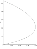
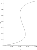
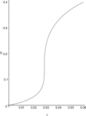
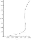
Figure 10. The algebraic function $S(t)$ and some of its conjugates, for $\nu=0.5$, $\nu=1.1$, $\nu=\nu_{c}$ and $\nu=8$. The function $S$ is the branch that vanishes at the origin. The values of $t$ where the tangent is vertical are such that $P_{1}(\nu,t)=0$ or $P_{2}(\nu,t)=0$. The form of the function is in agreement with the fact that the radius of $S$ is given in Figure 9 by the highest of the curves.

12.2. Two-colored triangulations

Theorem 23.

The Potts generating function of quasi-triangulations $Q(2,\nu,t,w,z;x,y)$, defined by (23) and taken at $q=2$, is algebraic.

In particular, the series $Q_{i}(2,\nu,t):=[y^{i}]Q(2,\nu,t,1,1;0,y)$ that counts two-colored near-triangulations of outer degree $i$ by edges ($t$) and monochromatic edges ($\nu$) is algebraic of degree (at most) $5$ over ${\mathbb{Q}}(\nu,t)$ and admits a rational parametrisation. Set $v=(\nu+1)/(\nu-1)$. Let $S\equiv S(\nu,t)$ be the unique power series in $t$ having constant term $v$ and satisfying

$$t^{3}={\frac{\left(S-v\right)\left(S-2+v\right)\left(2\,v-{v}^{2}+2\,S+{S}^{2}-4\,{S}^{3}\right)}{64\left(1+v\right)^{3}{S}^{2}}}.$$ (99)

Then $t^{i}Q_{i}(2,\nu,t)$ has a rational expression in terms of $S$ and $v$. In particular,

$$t^{4}Q_{1}(2,\nu,t)=t^{5}\nu Q_{2}(2,\nu,t)={\frac{\left(S-v\right)^{2}\left(S-2+v\right)\left(-2\,v+{v}^{2}-Sv-{S}^{2}v+3\,{S}^{3}\right)}{128\left(1+v\right)^{4}{S}^{2}}},$$

while

$$t^{6}Q_{3}(2,\nu,t)=\frac{(S-v)^{3}(S-2+v)P(v,S)}{8192(1+v)^{6}S^{4}}$$

with

$$P(v,S)=-64\,{S}^{6}+\left(232-128\,v\right){S}^{5}-\left(67+48\,v-64\,{v}^{2}\right){S}^{4}+\left(106-102\,v+40\,{v}^{2}\right){S}^{3}\\ -2\,\left(v-2\right)\left(32\,{v}^{2}-48\,v-1\right){S}^{2}+2\,\left(3\,v-1\right)\left(v-2\right)^{2}S+3\,v\left(v-2\right)^{3}.$$

Proof.

The first statement is a specialization of Theorem 18. Recall that the variables $w$ and $z$ are redundant: we thus focus on the case $w=z=1$. To obtain explicit algebraic equations for near-triangulations, we first construct an equation with one catalytic variable satisfied by $Q(y)\equiv Q(0,y)$, as described in Section 11.

We write the invariant equation (42) for $q=2$ and $m=4$. It involves five unknown series $C_{0},\ldots,C_{4}$, independent of $y$. By expanding this equation in the neighborhood of $y=0$ and writing that the coefficient of $y^{-2r}$ is zero, we obtain explicit expressions for the series $C_{r}$, as described in Section 11.2.1. Moreover, by writing that the coefficient of $y^{-2r+1}$ is zero, for $1\leq r\leq 4$, we obtain additional identities relating the series $Q^{(i)}(0)$. More precisely:

• by extracting the coefficients of $y^{-8}$, $y^{-6}$, $y^{-4}$, we obtain:

  $$C_{4} = -4\nu^{4},$$

  $$C_{3} = 8\,{\nu}^{2}\left(\nu-1\right)\left(2\,\nu-3\right),$$

  $$C_{2} = 16\,{\nu}^{3}\left(\nu-1\right){t}^{3}+4\,\left(5\,\nu+1\right)\left(\nu-1\right)^{3};$$

• extracting the coefficients of $y^{-7}$ and $y^{-5}$ does not yield new identities;

• extracting the coefficient of $y^{-3}$ gives $Q(0)=1$, which is not a surprise. From now on we systematically replace every occurrence of $Q(0)$ by $1$;

• extracting the coefficient of $y^{-2}$ gives

  $$C_{1}=-64\,{\nu}^{2}\left(\nu-1\right)^{2}{t}^{4}Q^{\prime}(0)+48\,\nu\,\left(\nu-1\right)^{2}{t}^{3}+4\,\left(2\,\nu-1\right)\left(\nu-1\right)^{3};$$

• extracting the coefficient of $y^{-1}$ gives:

  $$Q^{\prime\prime}(0)=\frac{2Q^{\prime}(0)}{t\nu}.$$ (100)

  This identity is a special case of the last statement of Proposition 2, and has a simple combinatorial explanation. From now on we systematically replace every occurrence of $Q^{\prime\prime}(0)$ by this expression;

• finally, extracting the coefficient of $y^{0}$ gives

  $$C_{0}=-{\frac{32}{3}}\,{\nu}^{2}\left(\nu-1\right)^{2}{t}^{6}Q^{(3)}(0)-32\,\left(\nu+1\right)\left(\nu-2\right)\left(\nu-1\right)^{2}{t}^{4}Q^{\prime}(0)\\ -112\,{\nu}^{2}\left(\nu-1\right)^{2}{t}^{6}-8\,\left(\nu-4\right)\left(\nu-1\right)^{3}{t}^{3}+\left(\nu-1\right)^{4}.$$

Let us now replace each $C_{r}$ by its expression in the invariant equation (42): this gives, after dividing by $32(\nu-1)^{3}t^{3}$, an equation with one catalytic variable for $Q(y)$, of the form (80), involving the (only) two unknown series $Q^{\prime}(0)$ and $Q^{(3)}(0)$.

To solve this equation and obtain an algebraic equation satisfied by $Q^{\prime}(0)$, we can use the general strategy of [12]. But we can also apply the alternative method already used for 2-colored planar maps in the previous subsection. Consider the following two polynomials in $X$:

$$P_{\pm}(X):=\sum_{r=0}^{4}C_{r}(tX)^{r}\pm\left(2\nu^{2}{t}^{2}X^{2}+\beta\left(4\beta+2\right)tX-4\beta\nu{t}^{3}+\beta^{2}\right)^{2}$$

where $\beta=\nu-1$. The second term is simply the square of the series $D(y)$ defined in Proposition 8, seen as a polynomial in $X\equiv I(y)$. Then the polynomials $P_{+}(X)$ and $P_{-}(X)$ have a double root in $X$. Hence the discriminant of each of them vanishes. This gives two polynomial equations relating $Q^{\prime}(0)$ and $Q^{(3)}(0)$, from which we obtain an equation of degree 5 for $Q_{1}(2,\nu,t)\equiv Q^{\prime}(0)$ by elimination. The genus of the corresponding curve (in $t$ and $Q^{\prime}(0)$) is found to be $0$, so that the curve has a rational parametrization, which we have constructed with the help of the algcurves package of Maple.

The expression of $Q_{2}(2,\nu,t)=Q^{\prime\prime}(0)/2$ follows from (100). The expression of $Q_{3}(2,\nu,t)=Q^{(3)}(0)/6$ can be obtained using any of the polynomial equations relating $Q^{\prime}(0)$ and $Q^{(3)}(0)$ that we have obtained on the way to our derivation of $Q^{\prime}(0)$.

Let us finally explain why each series $t^{i}Q_{i}(2,\nu,t)$ can be written in terms of $S$ and $v$. The equation with one catalytic variable satisfied by $Q(y)$ reads

$$6t^{3}\nu^{2}(Q(y)-1)=y\,\operatorname{Pol}(\nu,Q(y),Q_{1},Q_{3},t,y)$$

for some polynomial $\operatorname{Pol}$ with integer coefficients. Differentiating $i$ times with respect to $y$, and then setting $y=0$ thus gives $Q^{(i)}(0)\equiv i!\,Q_{i}(2,\nu,t)$ as a polynomial in $Q_{1},\ldots,Q_{i-1}$ with coefficients in ${\mathbb{Q}}(\nu,t)$. By combining Euler’s relation and the edge/face incidence relation, one easily shows that $t^{i}Q_{i}(2,\nu,t)$ is a series in $t^{3}$. Since $\nu$ can be expressed in terms of $v$, and $t^{3},Q_{1},Q_{2},Q_{3}$ can be expressed rationally in terms of $v$ and $S$, the same holds for any $t^{i}Q_{i}(2,\nu,t)$ by induction on $i$.  

Connections with previous work. This result is very close to the solution of the Ising model on near-cubic maps, derived by Boulatov & Kazakov [9] using matrix integrals and then by Bousquet-Mélou & Schaeffer [15] using bijections with trees. We say that a planar map is near-cubic if its dual is a near-triangulation; that is, every non-root vertex has degree 3. Then for a generic value of $q$, the series $Q_{i}(q,\nu,t):=[y^{i}]Q(q,\nu,t,1,1;0,y)$, which counts $q$-colored near-triangulations of outer degree $i$ by edges and monochromatic edges, can be interpreted in terms of near-cubic maps using the duality relation (18):

$$Q_{i}(q,\nu,t) = \sum_{M\rm{near-triang.}\atop\operatorname{df}(M)=i}t^{\operatorname{e}(M)}\operatorname{P}_{M}(q,\nu)$$ (101)

$$= \sum_{G\,\rm{near-cubic}\atop\operatorname{dv}(G)=i}t^{\operatorname{e}(G)}\operatorname{P}_{G^{*}}(q,\nu)$$

$$= \sum_{G\,\rm{near-cubic}\atop\operatorname{dv}(G)=i}t^{\operatorname{e}(G)}\,\frac{(\nu-1)^{\operatorname{e}(G)}}{q^{\operatorname{v}(G)-1}}\operatorname{P}_{G}\left(q,1+\frac{q}{\nu-1}\right)\hskip 85.35826pt\hbox{by~{}\eqref{eq:duality-Potts-poly}}$$

$$= \left(\frac{t(\nu-1)}{q}\right)^{-i}\sum_{G\,\rm{near-cubic}\atop\operatorname{dv}(G)=i}\left(\frac{(\nu-1)^{3}t^{3}}{q^{2}}\right)^{\operatorname{f}(G)-1}\operatorname{P}_{G}\left(q,1+\frac{q}{\nu-1}\right).$$

We have used in the last line Euler’s relation and the edge/vertex incidence relation, according to which $2\operatorname{e}(G)=3(\operatorname{v}(G)-1)+\operatorname{dv}(G)$.

Let us return to the case $q=2$. The series $I_{i}(X,u)$ studied in [15] counts by non-root vertices (variable $X$) and by bichromatic edges (variable $u$) 2-colored near-cubic maps $G$ such that $\operatorname{dv}(G)=i$ (as in the present paper, the color of the root vertex is fixed). The connection between our series $Q_{i}(2,\nu,t)$ follows from (101):

$$Q_{i}(2,\nu,t)=\left(\frac{t(\nu-1)}{2}\right)^{-i}(uX)^{i}I_{i}(X,u)$$

with

$$u=\frac{\nu-1}{\nu+1},\quad\quad X^{2}=\frac{(\nu+1)^{3}t^{3}}{4}.$$

Via this correspondence, the value of $Q_{2}(2,\nu,t)$ given in Theorem 23 is equivalent to the case $X=Y$ of [15, Proposition 20]. The series $\bar{Q}$ defined in the latter reference coincides with the series $S$ defined by (99).

Singularity analysis. The singular behaviour of $Q_{1}(2,\nu,t)$ is similar to that of the series $M(2,\nu,t,1,1;1,1)$ studied in the previous subsection. Again, we state our results without proof (see also [9]).

Claim 24.

Let $P_{1}$ and $P_{2}$ be the following two polynomials:

$$P_{1}(\nu,\rho)\ =\ 131072\,{\rho}^{3}{\nu}^{9}-192\,{\nu}^{6}\left(3\,\nu+5\right)\left(\nu-1\right)\left(3\,\nu-11\right){\rho}^{2}\\ -48\,{\nu}^{3}\left(\nu-1\right)^{2}\rho+\left(\nu-1\right)\left(4\,{\nu}^{2}-8\,\nu-23\right),$$

$$P_{2}(\nu,\rho)\ =\ 27648\,{\rho}^{2}{\nu}^{4}+864\,\nu\,\left(\nu-1\right)\left({\nu}^{2}-2\,\nu-1\right)\rho+\left(7\,{\nu}^{2}-14\,\nu-9\right)\left(\nu-2\right)^{2}.\hskip 71.13188pt$$

Consider $tQ_{1}(2,\nu,t)$ as a series in $t^{3}$ depending on the parameter $\nu$. Let $\rho_{\nu}$ denote its radius of convergence. Then $\rho_{\nu}$ is a continuous decreasing function of $\nu$ for $\nu>0$, which satisfies

$$\begin{array}[]{lllllll}P_{2}(\nu,\rho_{\nu})&=&0&\hbox{for}&0<\nu\leq\nu_{c}:=1+1/\sqrt{7},\\ P_{1}(\nu,\rho_{\nu})&=&0&\hbox{for}&\nu_{c}\leq\nu.\end{array}$$

Moreover,

$$\rho_{\nu}\rightarrow+\infty\ \hbox{ as }\nu\rightarrow 0\quad\hbox{ and }\quad\rho_{\nu_{c}}=\frac{25\,\sqrt{7}-55}{864}.$$

The critical behaviour of $tQ_{1}(2,\nu,t)$ is usually the standard behaviour of planar maps series, with an exponent $3/2$:

$$tQ_{1}(2,\nu,t)=\alpha_{\nu}+\beta_{\nu}(1-t^{3}/\rho_{\nu})+\gamma_{\nu}(1-t^{3}/\rho_{\nu})^{3/2}\,(1+o(1)),$$

except at $\nu=\nu_{c}$, where the nature of the singularity changes:

$$tQ_{1}(2,\nu_{c},t)=\alpha_{\nu_{c}}+\beta_{\nu_{c}}(1-t^{3}/\rho_{\nu_{c}})+\gamma_{\nu_{c}}(1-t^{3}/\rho_{\nu})^{4/3}\,(1+o(1)).$$

Note. The analysis is similar to the case of general planar maps, but the role that was played by the series $S$ in the proof of Claim 22 is now played by the series $U$ such that $S=v(1-2U)$. In particular, $U$ has constant term 0 and non-negative coefficients (which is not the case of $S$).

13. Three colors

In this section, we focus on the case $k=1$, $m=6$, that is, on $q=3$. We give explicit algebraic equations satisfied by generating functions of properly 3-colored planar maps and triangulations. This corresponds to $\nu=0$. The case when $\nu$ is generic leads to equations with one catalytic variable involving four unknown series (of the form $M^{(i)}(1)$ or $Q^{(i)}(0)$, depending on whether we deal with general maps or triangulations), and their solution has defeated us so far. However, we conjecture an algebraic equation for the series counting properly 3-colored cubic maps (Conjecture 27).

13.1. Three-colored planar maps

Theorem 25.

The Potts generating function of planar maps $M(3,\nu,t,w,z;x,y)$, defined by (19) and taken at $q=3$, is algebraic.

The specialization $M(3,0,t,1,1;1,1)$ that counts properly three-colored planar maps by edges has degree $4$ over ${\mathbb{Q}}(t)$, and admits a rational parametrization. Let $S\equiv S(t)$ be the unique power series in $t$ with constant term $0$ satisfying

$$t=\frac{S(1-2\,S^{3})}{\left(1+2S\right)^{3}}.$$ (102)

Then

$$M(3,0,t,1,1;1,1)={\frac{\left(1+2\,S\right)\left(1-2\,{S}^{2}-4\,{S}^{3}-4\,{S}^{4}\right)}{\left(1-2\,{S}^{3}\right)^{2}}}.$$ (103)

The coefficient of $t^{n}$ in this series, which is the number of properly $3$-colored maps with $n$ edges, is asymptotic to $\kappa\,\mu^{n}n^{-5/2},$ where

$$\kappa>0\quad\hbox{and}\quad\mu=\frac{22+8\,\sqrt{6}}{3}.$$

Proof.

The first statement is a specialization of Theorem 15. We would like to obtain an explicit equation satisfied by $M(3,\nu,t,w,z;1,1)$. As described in Section 10, we first construct an equation with one catalytic variable satisfied by $M$. Once again, the variable $z$ is redundant, and we set $z=1$.

An equation with one catalytic variable. We start from the invariant equation (41), written for $q=3$ and $m=6$. It involves seven unknown series $C_{0},\ldots,C_{6}$, independent of $y$. By expanding this equation in the neighborhood of $y=1$, as described in Section 10.2.1, we obtain explicit expressions of the series $C_{r}$. More precisely,

• $C_{6},C_{5}$ and $C_{4}$ are polynomials in $\nu$, $t$ and $w$,

• $C_{3}$ is a polynomial in $\nu$, $t$, $w$ and $M(1)$,

• $C_{2}$ is a polynomial in $\nu$, $t$, $w$, $M(1)$ and $M^{\prime}(1)$,

• $C_{1}$ is a polynomial in $\nu$, $t$, $w$, $M(1)$, $M^{\prime}(1)$ and $M^{\prime\prime}(1)$,

• $C_{0}$ is a polynomial in $\nu$, $t$, $w$, $M(1)$, $M^{\prime}(1)$, $M^{\prime\prime}(1)$ and $M^{(3)}(1)$.

In the invariant equation (41), let us now replace each $C_{r}$ by its expression : as was proved for general values of $k$ and $m$ in Section 10.2.2, this gives, after dividing by

$$27tw(\nu-1)^{2}\,\left(1-\bar{y}\right)\left(1-\nu+\bar{y}+\nu\bar{y}\right)\left(1-\nu+2\bar{y}+\nu\bar{y}\right)\left(2-2\nu+\bar{y}+2\,\nu\bar{y}\right),$$

an equation with one catalytic variable of the form (63), involving the series $M(1)$, $M^{\prime}(1)$, $M^{\prime\prime}(1)$ and $M^{(3)}(1)$, that is, the first four discrete derivatives of $M(y)$. Even though the general strategy of [12] allows one to solve, in theory, this equation, the size of the calculations has prevented us to do so in the general case.

So let us focus on the simpler case of properly three-colored planar maps. That is, we set $\nu=0$ so as to forbid monochromatic edges. This simplifies the series $C_{r}$. Indeed, $C_{3}$ (resp. $C_{2}$, $C_{1}$, $C_{0}$) does not involve $M(1)$ (resp. $M^{\prime}(1)$, $M^{\prime\prime}(1)$, $M^{(3)}(1))$ any more. We further ignore the number of vertices by setting $w=1$. The resulting equation in one catalytic variable reads

$$\operatorname{Pol}(M(y),M(1),M^{\prime}(1),M^{\prime\prime}(1),t;y)=0,$$ (104)

and has degree 4 in $M(y)$. More precisely, the equation can be written

$$M(y)=1+\frac{ty^{2}}{2\left(2\,y+1\right)\left(y+2\right)\left(y+1\right)}P(M(y),\Delta M(y),\Delta^{2}M(y),\Delta^{3}M(y),t,y)$$ (105)

where

$$P(x_{0},x_{1},x_{2},x_{3},t,y)=1+11\,y+4\,{t}^{2}{y}^{2}x_{{3}}+2\left(-13\,{y}^{2}+2\,{t}^{2}{y}^{2}+5\,t{y}^{2}-29\,y-2\,ty-9\right)x_{{0}}\\ +\left(8\,{y}^{3}+2\,t{y}^{3}+32\,{t}^{2}{y}^{3}-62\,t{y}^{2}+54\,{y}^{2}+32\,{t}^{2}{y}^{2}-12\,ty+75\,y+25\right){x_{{0}}}^{2}\\ +2\,t{y}^{2}\left(-26\,{y}^{2}+42\,t{y}^{2}+36\,ty-65\,y-26+18\,t\right){x_{{0}}}^{3}+36\,{t}^{2}{y}^{4}\left(2\,y+1\right){x_{{0}}}^{4}\\ +2\left(6\,{t}^{2}{y}^{2}-4\,t{y}^{2}+16\,{y}^{2}+9\,y-4\,ty+2\right)x_{{1}}-2\,ty\left(22\,t{y}^{2}-33\,{y}^{2}-34\,ty+27\,y+6\right){x_{{1}}}^{2}\\ +36\,{t}^{2}{y}^{2}\left(y-1\right)^{2}{x_{{1}}}^{3}+2\,ty\left(18\,t{y}^{2}-27\,{y}^{2}+50\,ty-78\,y-12\right)x_{{0}}x_{{1}}+36\,{y}^{2}\left({y}^{2}+2\,y+3\right){t}^{2}x_{{1}}{x_{{0}}}^{2}\\ -36\,{y}^{2}\left(y+3\right)\left(y-1\right){t}^{2}x_{{0}}{x_{{1}}}^{2}+2\,ty\left(6\,ty-11\,y-2\right)x_{{2}}+12\,{y}^{2}\left(y+3\right){t}^{2}x_{{0}}x_{{2}}-36\,\left(y-1\right){y}^{2}{t}^{2}x_{{1}}x_{{2}}.$$

Still, both the general approach of [12] and Tutte’s alternative (used above for two-colored planar maps) require heavy calculations. Hence we have resorted to Tutte’s good old method: guess and check!

An interlude: solving planar maps by guessing and checking. Because things are so heavy with our equation, let us discuss the principles of this method on the much simpler example of planar maps counted by edges (variable $t$) and outer degree (variable $y$). The standard equation with one catalytic variable that defines the associated generating function $G(t;y)\equiv G(y)$ reads

$$G(y)=1+ty^{2}G(y)^{2}+ty\,\frac{yG(y)-G(1)}{y-1}.$$ (106)

It is clear that this equation has a unique solution that is a power series in $t$. The coefficients of this series are polynomials in $y$. But how can we determine $G(y)$? Assume that we find two series, $F(t;y)\equiv F(y)\in{\mathbb{Q}}[y][[t]]$ and $F_{0}(t)\equiv F_{0}\in{\mathbb{Q}}[[t]]$, such that

$$F(y)=1+ty^{2}F(y)^{2}+ty\,\frac{yF(y)-F_{0}}{y-1}.$$ (107)

Then, by multiplying by $(y-1)$ and setting $y=1$, we discover that $F_{0}$ equals necessarily $F(1)$, so that $F(y)$ is the map generating function $G(y)$. Note that it is important that the series $F(y)$ has polynomial coefficients in $y$ (or at least, coefficients in ${\mathbb{Q}}(y)$ having no pole at $y=1$). Otherwise $F(1)$ may not be well-defined.

From the functional equation (106), one can compute the first coefficients of the series $G(y)$. In particular, one can easily conjecture, using tools like the Gfun package of Maple [44], that $G(1)$ is quadratic:

$$27\,{t}^{2}G(1)^{2}+G(1)(1-18\,t)-1+16\,t=0.$$

The corresponding curve has genus 0, and thus admits a rational parametrization. Let $S\equiv S(t)$ be the unique power series in $t$ satisfying $S=t(1+3S)^{2}$. Then our conjectured value of $G(1)$ is $G(1)=(1-S)(1+3S).$ Let us define $F_{0}:=(1-S)(1+3S)$. There exists a unique power series $F(y)\equiv F(t;y)$ satisfying (107) (indeed, this equation is quadratic in $F(y)$, and the other root contains negative powers of $t$). However, this series has a priori coefficients in ${\mathbb{Q}}(y)$. We wish to prove these coefficients actually lie in ${\mathbb{Q}}[y]$. One way goes as follows. In (107), replace $F_{0}$ by its value $(1-S)(1+3S)$, and $t$ by its expression $t=S/(1+3S)^{2}$. As a curve in $F(y)$ and $y$ over ${\mathbb{Q}}(S)$, the resulting equation has genus 0 again, and thus admits a rational parametrization. Indeed, let $W$ be the unique series in ${\mathbb{Q}}[y][[t]]$ satisfying

$$W=y\,\frac{1+SW+S(S+1)W^{2}}{1+3S}.$$

Then

$$F(y)={\frac{\left(1-S(1+S)W\right)\left(1+SW+S(S+1){W}^{2}\right)}{1-SW}}.$$

This expression shows that $F(y)$ has polynomial coefficients in $y$, and we have proved that $F(y)$ is the generating function $G(y)$ of planar maps.

Back to 3-colored planar maps. Let us return to the functional equation (104–105). It defines a unique series $M(y)\equiv M(t;y)\in{\mathbb{Q}}(y)[[t]]$. Moreover, the form of the equation implies that the coefficient of $t^{n}$ in this series has no pole at $y=1$. (For combinatorial reasons, we know that the coefficients are polynomials in $y$, but the form of the equation does not imply such a strong statement). Assume we find 4 series, $F(t;y)\equiv F(y)\in{\mathbb{Q}}[y][[t]]$, and $F_{0},F_{1},F_{2}\in{\mathbb{Q}}[[t]]$, such that

$$\operatorname{Pol}(F(y),F_{0},F_{1},F_{2},t;y)=0.$$

By expanding this identity in the neighborhood of $y=1$, it follows that $F_{0}=F(1)$, $F_{1}=F^{\prime}(1)$ and $F_{2}=F^{\prime\prime}(1)$ (the derivatives being taken with respect to $y$). Consequently, the series $F(y)$ satisfies the same equation as $M(y)$, and $F(y)=M(y)$.

So our first task is to guess the values of $F^{(i)}(1)$, for $0\leq i\leq 2$. From the functional equation (1) one can compute the first coefficients of the series $M(y)=M(3,0;t,1;1,y)$. The first 40 coefficients of $M_{0}:=M(1)$ suffice to conjecture that this series satisfies

$$-12500\,{t}^{6}M_{0}^{4}-24\,{t}^{4}\left(71-1000\,t\right)M_{0}^{3}-2\,{t}^{2}\left(39-1020\,t+7216\,{t}^{2}+3600\,{t}^{3}\right)M_{0}^{2}\\ -M_{0}\,\left(1-42\,t+536\,{t}^{2}-1712\,{t}^{3}-9040\,{t}^{4}+864\,{t}^{5}\right)+1-40\,t+540\,{t}^{2}-2720\,{t}^{3}+432\,{t}^{4}=0.$$

The corresponding curve has genus $0$, and the parametrization by the series $S$ given in the theorem is constructed using Maple.

We now compute more coefficients of $M(y)$, in order to conjecture the values of $M^{\prime}(1)$ and $M^{\prime\prime}(1)$. In the expansions of these two series, we systematically replace the variable $t$ by its expression (102) in terms of $S$, as we suspect that $M^{\prime}(1)$ and $M^{\prime\prime}(1)$ will have a high degree over ${\mathbb{Q}}(t)$, but hopefully a smaller degree over ${\mathbb{Q}}(S)$. And indeed, from the first 80 terms of $M(y)$ (and of course with the help of Maple), we conjecture that $M^{\prime}(1)$ is quadratic over ${\mathbb{Q}}(S)$:

$$M^{\prime}(1)={\frac{\left(1+2\,S\right)\left(P(S)+Q(S)\sqrt{(1+2S)(1+2S+4S^{2})}\right)}{{S}^{2}\left(1-2\,{S}^{3}\right)^{4}}}$$

with

$$P(S)=32\,{S}^{12}+32\,{S}^{11}+12\,{S}^{10}-32\,{S}^{9}-16\,{S}^{8}+18\,{S}^{7}+14\,{S}^{6}-28\,{S}^{5}-58\,{S}^{4}-49\,{S}^{3}-25\,{S}^{2}-7\,S-1$$

and

$$Q(S)=\left(1-2\,{S}^{3}\right)\left(1+2S+4\,{S}^{2}\right)\left(1+S\right)^{3}.$$

Hoping that $M^{\prime\prime}(1)$ lies in the same quadratic extension of ${\mathbb{Q}}(S)$ as $M^{\prime}(1)$, we then look for a linear relation between $1$, $M^{\prime}(1)$ and $M^{\prime\prime}(1)$ with polynomial coefficients in $S$ (using the command hermite_pade) and obtain the conjectured expression:

$$M^{\prime\prime}(1)={\frac{2\left(1+2\,S\right)\left(\bar{P}(S)+\bar{Q}(S)\sqrt{(1+2S)(1+2S+4S^{2})}\right)}{{S}^{3}\left(1-2\,{S}^{3}\right)^{6}}}$$

with

$$\bar{P}(S)=-5-54\,S-300\,{S}^{2}-1082\,{S}^{3}-2721\,{S}^{4}-4768\,{S}^{5}-5310\,{S}^{6}-1944\,{S}^{7}+4970\,{S}^{8}+10468\,{S}^{9}\\ +8724\,{S}^{10}+12\,{S}^{11}-8336\,{S}^{12}-10080\,{S}^{13}-6016\,{S}^{14}-1728\,{S}^{15}+96\,{S}^{16}-64\,{S}^{17}-192\,{S}^{18}-192\,{S}^{19}$$

and

$$\bar{Q}(S)=\left(1+S\right)^{3}\left(1-2\,{S}^{3}\right)\left(1+2\,S+4\,{S}^{2}\right)\times\\ \left(8{S}^{7}+8\,{S}^{6}+12\,{S}^{5}-20\,{S}^{4}-48\,{S}^{3}-42\,{S}^{2}-19\,S-5\right).$$

Now return to (104). Consider the quartic equation (in $F(y)$):

$$\operatorname{Pol}\left(F(y),F_{0},F_{1},F_{2},\frac{S(1-2S^{3})}{(1+2S)^{3}};y\right)=0,$$ (108)

where $F_{0}$ (resp. $F_{1}$, $F_{2}$) is the conjectured value of $M(1)$ (resp. $M^{\prime}(1)$, $M^{\prime\prime}(1)$). The rational function of $S$ that occurs is just the expression (102) of $t$ in terms of $S$. When $S=0$, this equation has degree 1 in $F(y)$. Hence (108) admits a unique solution in ${\mathbb{Q}}(y)[[t]]$, denoted $F(y)\equiv F(t;y)$. As argued above, if we can prove that this series has coefficients in ${\mathbb{Q}}[y]$ (or that its coefficients have no pole at $y=1$), we can conclude that $F(y)=M(y)$, and that the conjectured values of $M(1)$, $M^{\prime}(1)$ and $M^{\prime\prime}(1)$ are correct.

With the help of the parametrization function of Maple, and of an extension of it provided by Mark van Hoeij, we have discovered that the quartic equation (108), seen as a curve in $y$ and $F(y)$ over ${\mathbb{Q}}(S,\sqrt{(1+2S)(1+2S+4S^{2})})$, admits a rational parametrization which we now describe. Set $T=2S$, $\Delta=(1+T)(1+T+T^{2})$, and consider the following quartic equation in $W$:

$$W=y\,\frac{P_{1}+P_{2}\,\sqrt{\Delta}}{2(1-TW)(2-TW)(1+T)^{2}\left((1+T+T^{2})(1-TW)+\sqrt{\Delta}\right)}$$ (109)

where

$$P_{1}=(1+T)(1+T+T^{2})\left(4-12\,TW-\left(9\,T+4\right)T^{2}W^{3}+3\left(T+1\right)T^{3}W^{4}+2\left(7\,T+1\right)TW^{2}\right)$$

and

$$P_{2}=-\left(T+1\right)^{3}T^{3}W^{4}+\left(T+1\right)\left(T-4\right)T^{2}W^{3}+\left(5\,{T}^{3}+8\,T^{2}+14\,T+6\right)TW^{2}\\ -2\,\left(3\,T^{2}+5\,T+6\right)TW+2\,T^{2}+4\,T+4.$$

Recall that at $t=0$, the series $S$ and $T$ vanish. This implies that (109) defines a unique series $W\in{\mathbb{Q}}[y][[t]]$. Now in (108), let us replace $S$ by $2T$ and $y$ by its rational expression in terms of $T$, $\sqrt{\Delta}$ and $W$ derived from (109). We leave it to the reader’s computer algebra system to check that (108) then factors into a factor of degree 3 in $F(y)$, and a linear one. Moreover, setting $t=0$ (that is, $T=0$) shows that the linear factor is the only one that has a solution $F(y)\in{\mathbb{Q}}(y)[[t]]$. Solving it for $F(y)$ gives

$$F(y)=\frac{P_{3}(T,\sqrt{\Delta},W)}{P_{4}(T,\sqrt{\Delta},W)}$$

for two polynomials $P_{3}$ and $P_{4}$ with coefficients in ${\mathbb{Q}}$, such that $P_{4}(0,1,W)$ (which is the value taken by $P_{4}$ when $T=0$) lies in ${\mathbb{Q}}$ and is non-zero. This shows that $F(y)$ belongs to ${\mathbb{Q}}[y][[t]]$. This completes our very long proof of the short equation (103).

A simple singularity analysis [27, Chap. VII.7] of $M(3,0,t,1,1;1,1)$ yields the asymptotic behaviour of the number of $3$-colored planar maps with $n$ edges.  

13.2. Three-colored triangulations

By Theorem 18, the series $Q(3,\nu,t,w,z;x,y)$ is algebraic. Without loss of generality, we can set $w=z=1$. We can also focus on near-triangulations (no digon allowed) by considering $Q(y)\equiv Q(3,\nu,t,1,1;0,y)$. This series counts three-colored near-triangulations by edges (variable $t$), monochromatic edges (variable $\nu$) and outer degree (variable $y)$. It is algebraic over ${\mathbb{Q}}(\nu,t,y)$.

In what follows, we first describe the construction of the equation with one catalytic variable satisfied by $Q(y)$. Alas, it involves four unknown series $Q^{(i)}(0)$, and we have not succeeded in solving it for a generic value of $\nu$. We solve it, however, for $\nu=0$, thus counting proper colourings of near-triangulations. But this result can probably be obtained by simpler means. Due to the duality relation (101), another interesting case is $\nu=-2$, for which our series actually counts proper 3-colorings of near-cubic maps. We have not solved the equation in this case, but we state a conjecture for its solution, due to Bruno Salvy (and obtained by computing many coefficients of the solution).

We start from the invariant equation (42), written for $q=3$ and $m=6$. It involves 7 unknown series $C_{0},\ldots,C_{6}$, which are independent of $y$. By expanding this equation in the neighborhood of $y=0$ and writing that the coefficient of $y^{-2r}$ is zero, we obtain explicit expressions for the series $C_{r}$, as described in Section 11.2.1. Moreover, by writing that the coefficient of $y^{-2r+1}$ is zero, for $1\leq r\leq 6$, we obtain additional identities relating the series $Q^{(i)}(0)$. More precisely:

• by extracting the coefficients of $y^{-12}$, $y^{-10}$, $y^{-8}$, we obtain:

  $$C_{6} = -27\nu^{6},$$

  $$C_{5} = 27\,{\nu}^{4}\left(\nu-1\right)\left(2\,\nu-5\right),$$

  $$C_{4} = 9/2\,{\nu}^{2}\left(\nu-1\right)\left(18\,{t}^{3}{\nu}^{3}+35\,{\nu}^{3}-75\,{\nu}^{2}+30\,\nu+10\right);$$

• extracting the coefficients of $y^{-11}$ and $y^{-9}$ does not yield new identities;

• extracting the coefficient of $y^{-7}$ gives $Q(0)=1$, which is not a surprise. From now on we systematically replace every occurrence of $Q(0)$ by $1$;

• extracting the coefficient of $y^{-6}$ gives an expression of $C_{3}$ as a polynomial in $\nu$, $t$ and $Q^{\prime}(0)$;

• extracting the coefficient of $y^{-5}$ gives the standard identity between $Q^{\prime\prime}(0)$ and $Q^{\prime}(0)$:

  $$Q^{\prime\prime}(0)=\frac{2Q^{\prime}(0)}{t\nu}.$$ (110)

  From now on we systematically replace every occurrence of $Q^{\prime\prime}(0)$ by this expression;

• extracting the coefficient of $y^{-4}$ gives an expression of $C_{2}$ as a polynomial in $\nu$, $t$, $Q^{\prime}(0)$ and $Q^{(3)}(0)$;

• extracting the coefficient of $y^{-3}$ gives an expression of $Q^{(4)}(0)$ in terms of $\nu$, $t$, $Q^{(3)}(0)$ and $Q^{\prime}(0)$:

  $$Q^{(4)}(0)=-24\left(6+{\frac{1}{{t}^{3}{\nu}^{2}}}\right)Q^{\prime}(0)+4\,{\frac{\left(1+\nu\right)Q^{(3)}(0)}{\nu\,t}}+24\,{\frac{\nu+2}{\nu\,t}}.$$ (111)

• extracting the coefficient of $y^{-2}$ gives an expression of $C_{1}$ as a polynomial in $\nu$, $t$, $Q^{\prime}(0)$, $Q^{(3)}(0)$ and $Q^{(5)}(0)$;

• extracting the coefficient of $y^{-1}$ gives an expression of $Q^{(6)}(0)$ in terms of $Q^{(5)}(0)$, $Q^{(3)}(0)$ and $Q^{\prime}(0)$;

• finally, extracting the coefficient of $y^{0}$ gives an expression of $C_{0}$ as a polynomial in $\nu$, $t$, $Q^{\prime}(0)$, $Q^{(3)}(0)$, $Q^{(5)}(0)$ and $Q^{(7)}(0)$.

Let us now replace each $C_{r}$ by its expression in the invariant equation (42): this gives, after dividing by $54(\nu-1)^{5}t^{3}$, an equation with one catalytic variable for $Q(y)$, of the form (80), involving the series $Q^{\prime}(0)$, $Q^{(3)}(0)$, $Q^{(5)}(0)$ and $Q^{(7)}(0)$.

This is enough to conclude that $Q(3,\nu,t,1,1;0,y)$ is algebraic, but too big to be solved with the methods that are available at the moment. However, the case $\nu=0$ comes out very easily. As explained further down, this is, unfortunately, not very surprising.

Theorem 26.

The series $Q(3,0,t,1,1;0,y)$, which counts properly three-colored near-triangulations by edges (variable $t$), and outer degree (variable $y)$ is algebraic of degree $6$ over ${\mathbb{Q}}(t,y)$.

Let $Q_{i}(t):=[y^{i}]Q(3,0,t,1,1;0,y)$ be the series that counts (by edges) properly three-colored near-triangulations of outer degree $i$. Then $Q_{1}(t)=0$ and for $i\geq 2$, each $Q_{i}(t)$ is (at most) quadratic over ${\mathbb{Q}}(t)$ and admits a rational parametrization. Let $S\equiv S(t)$ be the unique series in $t$ satisfying

$$S=t^{3}(1+2S)^{2}.$$

Then $t^{i}Q_{i}(t)$ admits a rational expression in terms of $S$. In particular,

$$Q_{2}(t)=2t(1+S-S^{2})\quad\hbox{and}\quad Q_{3}(t)=2S(1-S).$$ (112)

Proof.

Let us set $\nu=0$ in the equation with one catalytic variable obtained by the above construction: this simply gives $Q^{\prime}(0)=0$, which is obvious because maps counted by this series have a loop. This also follows from (110). In order to obtain a non-trivial equation, we proceed as follows: we first replace $Q^{(3)}(0)$ by its expression in terms of $Q^{\prime}(0)$ and $Q^{(4)}(0)$ derived from (111), and then $Q^{\prime}(0)$ by its expression in terms of $Q^{\prime\prime}(0)$ derived from (110). We finally divide the resulting equation by $\nu$, and set $\nu=0$. This gives for properly 3-colored near-triangulations a much simpler equation, with only one unknown series $Q^{\prime\prime}(0)$:

$$4\,{y}^{5}{t}^{3}Q(y)^{3}+{y}^{2}t\left({t}^{2}-10\,ty-8\,{y}^{2}\right)Q(y)^{2}+\left(6\,{t}^{2}{y}^{3}+2\,ty-2\,{t}^{2}+4\,{y}^{2}\right)Q(y)\\ -{t}^{3}{y}^{2}-2\,ty+2\,{t}^{2}-4\,{y}^{2}+{y}^{2}{t}^{2}Q^{\prime\prime}(0)=0.$$ (113)

This equation is easily solved, using either the quadratic method, or the more general method of [12], and one obtains, with $Q_{2}=Q^{\prime\prime}(0)/2$:

$$8{t}^{5}\,Q_{2}^{2}+\left(1-12\,{t}^{3}-8\,{t}^{6}\right)Q_{2}-2\,t\left(1-11\,{t}^{3}-{t}^{6}\right)=0,$$

from which the first part of (112) easily follows.

For $i\geq 3$, (113) allows to compute $t^{2}Q_{i}(t)$ inductively as a polynomial in $t$ and the series $Q_{j}(t)$, for $2\leq j<i$.  

\begin{picture}(7054.0,2176.0)(2859.0,-3549.0)\end{picture}

Figure 11. A bipartite map and the corresponding Eulerian triangulation.

Remark. A triangulation admits a proper 3-coloring if and only if it is Eulerian, that is, if its faces are 2-colorable. The condition is necessary because each face of a properly 3-colored triangulation contains, in clockwise order, either the colors 1, 2, 3, or the colors 1, 3, 2, and two adjacent faces are of different types. That the condition is sufficient can be proved by induction on the face number. Moreover, Eulerian triangulation admits exactly 6 proper colorings. But there is a standard bijection between bipartite maps with $n$ edges and Eulerian triangulations with $3n$ edges, illustrated in Figure 11. Hence counting 3-colorable triangulations should not be harder than counting bipartite maps, which, as recalled in Section 2, can be done with a single catalytic variable by simply removing an edge (see (6)). Even though the 3-colorable near-triangulations considered here are a bit more general, it is not very surprising to find, for their enumeration, an equation with one catalytic variable and only one unknown series (see (113)).

A more exciting perspective is to obtain the generating function of properly 3-colored cubic maps. Indeed, according to (101),

$$Q_{i}(3,-2,t):=[y^{i}]Q(3,-2,t,1,1;0,1)=(-t)^{-i}\sum_{G\,\rm{near-cubic}\atop\operatorname{dv}(G)=i}(-3t^{3})^{\operatorname{f}(G)-1}\operatorname{P}_{G}\left(3,0\right).$$

Thus we have access in particular to the series

$$C(z):=\sum_{G\,\rm{near-cubic}\atop\operatorname{dv}(G)=1}z^{\operatorname{f}(G)}\operatorname{P}_{G}\left(3,0\right)=4\,{z}^{3}+84\,{z}^{4}+1872\,{z}^{5}+46464\,{z}^{6}+O\left({z}^{7}\right).$$

Fig. 12 justifies the value of the first two coefficients of this series. By computing recursively many coefficients of $C(z)$, and feeding Gfun with them, Bruno Salvy has reached the following rather formidable conjecture. How likely is it to hold? The equation below involves “only” 87 non-zero coefficients, while it holds at least up to order $O(z^{169})$. It holds significantly further modulo $p$ for numerous values of $p$, and so we believe it to be true.

Note that, in contrast with all solutions obtained so far, the genus of the corresponding curve is not 0, but 1. So we cannot hope for a rational parametrization.

Figure 12. The loopless near-cubic maps with root-degree 1 and 3 or 4 faces, and their number of proper 3-colorings (the color of the root is fixed). In each column, the first two maps correspond to the same graph.

Conjecture 27.

The generating function $C\equiv C(z)$ of properly $3$-colored near-cubic maps in which the degree of the root-vertex is $1$, counted by faces, is algebraic of degree $11$ and satisfies:

$$922337203685477580800000\,{C}^{11}+9007199254740992\,\left(194560000\,z-5971077\right){C}^{10}\\ +4294967296\,\left(280335535308800\,{z}^{2}-25398219177984\,z+446991689475\right){C}^{9}\\ -1024\,\left(379991218559385600000\,{z}^{4}-188284129271105978368\,{z}^{3}+74426563120993402880\,{z}^{2}\right.\\ \left.-3460024309515976704\,z+60644726921050599\right){C}^{8}\\ -1024\,\left(855256650185747464192\,{z}^{5}+198557240861845880832\,{z}^{4}+7030700057733103616\,{z}^{3}\right.\\ \left.-2005025500677518336\,{z}^{2}+65719379546147724\,z-1261082394855783\right){C}^{7}\\ -64\,\left(13794761675403801133056\,{z}^{6}+1749420037224685109248\,{z}^{5}-278771160986127695872\,{z}^{4}\right.\\ \left.+3443220359730862080\,{z}^{3}+294527021649617744\,{z}^{2}-12400864344288084\,z+586081179814293\right){C}^{6}\\ -16\,\left(32829338688610212249600\,{z}^{7}-541704013946292273152\,{z}^{6}-549137038895633924096\,{z}^{5}\right.\\ \left.+41876669882140680192\,{z}^{4}-936289577498747840\,{z}^{3}\right.\\ \left.+12987916499676352\,{z}^{2}+208517314053540\,z-54447680943015\right){C}^{5}\\ -32\,\left(124515522497539473408\,{z}^{9}+6242274275823592669184\,{z}^{8}-898808183791057633280\,{z}^{7}\right.\\ \left.-5275329284641325056\,{z}^{6}+6539785066149118976\,{z}^{5}-361493662811609868\,{z}^{4}\right.\\ \left.+9979948894517522\,{z}^{3}-432679480767965\,{z}^{2}+6248694091833\,z+378858660750\right){C}^{4}\\ -8\,\left(747093134985236840448\,{z}^{10}+5932367633073989222400\,{z}^{9}-1529736206124490686464\,{z}^{8}\right.\\ \left.+132585839072566050816\,{z}^{7}-3048630269218258944\,{z}^{6}-135087570198766176\,{z}^{5}\right.\\ \left.+5706147748413032\,{z}^{4}-229584590608200\,{z}^{3}+23755821897083\,{z}^{2}-152875558308\,z-27738626328\right){C}^{3}\\ +\left(-3361919107433565782016\,{z}^{11}-6012198464670331305984\,{z}^{10}+2332964327872863928320\,{z}^{9}\right.\\ \left.-341248528343609901056\,{z}^{8}+24933054438553903104\,{z}^{7}-994662704339242816\,{z}^{6}\right.\\ \left.+33270083406272816\,{z}^{5}-1608971168541300\,{z}^{4}+7467003627448\,{z}^{3}\right.\\ \left.+5037279798640\,{z}^{2}-194388001728\,z+808501760\right){C}^{2}\\ +z\,\left(-840479776858391445504\,{z}^{11}-157618519659107057664\,{z}^{10}+157170928122096254976\,{z}^{9}\right.\\ \left.-34691457904249143296\,{z}^{8}+3785139252232855552\,{z}^{7}-224694559056638912\,{z}^{6}\right.\\ \left.+6999136302319904\,{z}^{5}-197576502742812\,{z}^{4}+19551640345287\,{z}^{3}\right.\\ \left.-1347626230088\,{z}^{2}+40099744688\,z-404250880\right)C\\ -4\,{z}^{4}\left(19698744770118549504\,{z}^{9}-8025289374453202944\,{z}^{8}+1366977099830657024\,{z}^{7}\right.\\ \left.-120213529404735488\,{z}^{6}+5234026490678784\,{z}^{5}-86995002866345\,{z}^{4}\right.\\ \left.+4680668094111\,{z}^{3}-691486996440\,{z}^{2}+31610476208\,z-404250880\right)=0.$$

14. Non-separable maps

A map is separable if it is the atomic map $m_{0}$ (one vertex, no edge) or can be obtained by gluing two non-atomic maps at a vertex (more precisely, a corner of the first map is glued to a corner of the second map). Observe that both maps with one edge are non-separable.

Several authors have addressed the enumeration of families of colored non-separable planar maps. For instance, the series $T(x,y)$ defined by (1) and studied by Tutte in his long series of papers counts non-separable near-triangulations (all internal faces have degree 3). Also, Liu wrote a functional equation for the generating function of non-separable planar maps weighted by their Tutte polynomial [35], which was further studied by Baxter [3].

In this section, we first prove that the latter problem is equivalent to the enumeration of general planar maps (weighted, of course, by their Tutte polynomial). In particular, the algebraicity result of Theorem 15 translates into an algebraicity result for colored non-separable maps. Then, we show how Tutte’s equation (1) can be recovered from our equation (24) obtained for quasi-triangulations.

14.1. From general to non-separable planar maps

Let $\mathcal{N}$ be the set of non-separable planar maps and let $N(q,\nu,t,w,z;x,y)\equiv N(x,y)$ be the associated Potts generating function:

$$N(x,y)=\frac{1}{q}\sum_{N\in\mathcal{N}}t^{\operatorname{e}(N)}w^{\operatorname{v}(N)-1}z^{\operatorname{f}(N)-1}x^{\operatorname{dv}(N)}y^{\operatorname{df}(N)}\operatorname{P}_{N}(q,\nu).$$

The following proposition relates $N(x,y)$ to the Potts generating function  of general planar maps, denoted by $M(x,y)$ and defined by (19).

Proposition 28.

The series $M$ and $N$ are related by:

$$M(x,y)=1+\frac{M(1,1)M(x,y)}{M(x,1)M(1,y)}\,N\left(q,\nu,tM(1,1)^{2},w,z;x\frac{M(x,1)}{M(1,1)},y\frac{M(1,y)}{M(1,1)}\right)$$

where $M(x,y)\equiv M(q,\nu,t,w,z;x,y)$.

Proof.

A non-atomic map decomposes into a non-separable map (the core) containing the root-edge, in the corners of which are attached other rooted maps. This decomposition is illustrated in Figure 13. It induces a bijection between non-atomic maps and pairs consisting of a non-separable map $N$ (the core) and a ordered sequence of $2\operatorname{e}(N)$ maps $M_{1},\ldots,M_{2\operatorname{e}(N)}$ (since $2\operatorname{e}(N)$ is the number of corners of $N$).

\begin{picture}(15434.0,6020.0)(6203.0,-4784.0)\end{picture}

Figure 13. Decomposition of a map into a non-separable core in the corners of which are attached other maps.

Let $M$ be a non-atomic map and let $(N;M_{1},M_{2},\ldots,M_{2\operatorname{e}(N)})$ be its image by the decomposition. One clearly has

$$\operatorname{e}(M)=\operatorname{e}(N)+\sum_{i=1}^{2\operatorname{e}(N)}\operatorname{e}(M_{i}),$$

$$\operatorname{v}(M)=\operatorname{v}(N)+\sum_{i=1}^{2\operatorname{e}(N)}(\operatorname{v}(M_{i})-1),\quad\quad\operatorname{f}(M)=\operatorname{f}(N)+\sum_{i=1}^{2\operatorname{e}(N)}(\operatorname{f}(M_{i})-1),$$

and by (14) the Potts polynomial of $M$ is

$$\operatorname{P}_{M}(q,\nu)=\operatorname{P}_{N}(q,\nu)\prod_{i=1}^{2\operatorname{e}(N)}\frac{\operatorname{P}_{M_{i}}(q,\nu)}{q}.$$

Moreover, exactly $\operatorname{dv}(N)$ of the maps $M_{i}$ contribute to the degree $\operatorname{dv}(M)$ of the root-vertex of $M$. Similarly, $\operatorname{df}(N)$ of these maps contribute to the degree $\operatorname{df}(M)$ of the root-face of $M$. Finally, exactly one of these maps contributes to both $\operatorname{dv}(M)$ and $\operatorname{df}(M)$. These observations imply that $M(x,y)$ satisfies

$$M(x,y)=1+\frac{1}{q}\sum_{N\in\mathcal{N}}t^{\operatorname{e}(N)}w^{\operatorname{v}(N)-1}z^{\operatorname{f}(N)-1}x^{\operatorname{dv}(N)}y^{\operatorname{df}(N)}\operatorname{P}_{N}(q,\nu)\\ \times M(x,y)M(x,1)^{\operatorname{dv}(N)-1}M(1,y)^{\operatorname{df}(N)-1}M(1,1)^{2\operatorname{e}(N)-\operatorname{dv}(N)-\operatorname{df}(N)+1}$$

which yields the equation of the proposition.  

Corollary 29.

Let $q\not=0,4$ be of the form $2+2\cos j\pi/m$, with $j,m\in{\mathbb{Z}}$. Then the Potts generating function of non-separable planar maps, $N(q,\nu,t,w,z;x,y)$, is algebraic over ${\mathbb{Q}}(q,\nu,t,w,z;x,y)$.

Proof.

Let $s,u,v$ denote three indeterminates. Consider the following system:

$$T=s\,{M(T;1,1)}^{-2},$$

$$X=\displaystyle u\,\frac{M(T;1,1)}{M(T;X,1)},\quad\quad Y=\displaystyle v\,\frac{M(T;1,1)}{M(T;1,Y)},$$

where $M(t;x,y)$ stands for $M(q,\nu,t,w,z;x,y)$. Recall that $M(t;x,y)$ is a series in $t$ with coefficients in ${\mathbb{Q}}[q,\nu,w,z,x,y]$, satisfying $M(t;x,y)=1+O(t)$. This implies that the first equation defines $T$ uniquely as a series in $s$ with coefficients in ${\mathbb{Q}}[q,\nu,w,z]$. Moreover, $T=s+O(s^{2})$. Finally, the algebraicity of $M$ (Theorem 15) implies that of $T$. Indeed, if $P(t,M(t;1,1)^{2})=0$ for some non-trivial polynomial $P$ (with coefficients in ${\mathbb{Q}}(q,\nu,w,z)$), then $P(T,s/T)=0$ and $P(t,s/t)$ is not trivially $0$. Similarly, the second and third equations above respectively define $X$ and $Y$ as algebraic power series in $s$ with coefficients in ${\mathbb{Q}}(q,\nu,w,z,u)$ (resp. ${\mathbb{Q}}(q,\nu,w,z,v)$). By Proposition 28,

$$N(q,\nu,s,w,z;u,v)=\frac{M(T;X,1)M(T;1,Y)}{M(T;1,1)M(T;X,Y)}\left(M(T;X,Y)-1\right).$$ (114)

Given that each of the series $M$, $T$, $X$ and $Y$, is algebraic, $N(q,\nu,s,w,z;u,v)$ is algebraic over ${\mathbb{Q}}(q,\nu,s,w,z;u,v)$.  

The connection between the series $M$ and $N$ can be used to convert the functional equation (1) into a functional equation for $N$.

Corollary 30.

The Potts generating function $N(q,\nu,s,w,z;u,v)\equiv N(u,v)$ of non-separable planar maps satisfies:

$$N(u,v)=(q\!+\!\nu\!-\!1)\,swu{v}^{2}+\nu\,sz{u}^{2}v\\ \!\!\!\!\!\!+uvzs\frac{N(u,v)-vN(u,1)}{v-1-N(1,v)+vN(1,1)}+(\nu\!-\!1)\,uvws\frac{N(u,v)-uN(1,v)}{u-1-N(u,1)+uN(1,1)}.$$

Proof.

By specializing the equation of Proposition 28 to $x=1$ and/or $y=1$, one obtains:

$$M(x,1)=1+N(S;U,1),\quad\quad M(1,y)=1+N(S;1,V),\quad\quad M(1,1)=1+N(S;1,1)$$ (115)

with $N(s;u,v)\equiv N(q,\nu,s,w,z;u,v)$ and

$$S=t\,M(1,1)^{2},\quad U=x\,\frac{M(x,1)}{M(1,1)}\quad\hbox{ and }\quad V=y\,\frac{M(1,y)}{M(1,1)}.$$ (116)

This allows us to express $M(x,y)$ in terms of specializations of $N$:

$$M(x,y)=\left(1-\frac{1+N(S;1,1)}{(1+N(S;U,1))(1+N(S;1,V))}N(S;U,V)\right)^{-1},$$

Now, in the functional equation (1) defining $M(x,y)$, we replace the indeterminates $t$, $x$, $y$ by rational expressions of $S$, $U$, $V$ and specializations of $M$, using (116). Then, we use (115) and the above equation to express all occurrences of $M$ in terms of $N$. This gives the equation of the corollary, at $(s,u,v)=(S,U,V)$. Given that $t,x$ and $y$ can be recovered from $S$, $U$ and $V$ (using (116) and (115))), this equation must hold at a generic point $(s,u,v)$.  

Given the relation (16) between the Potts and Tutte polynomials, one can translate the equation for $N$ into an equation for the series

$$N\left((\mu-1)(\nu-1),\nu,t,\frac{w}{\nu-1},z;x,y\right)=\sum_{N\in\mathcal{N}}t^{\operatorname{e}(N)}w^{\operatorname{v}(N)-1}z^{\operatorname{f}(N)-1}x^{\operatorname{dv}(N)}y^{\operatorname{df}(N)}\operatorname{T}_{N}(\mu,\nu).$$

One thus recovers the equation of [36, Thm. 4.2], obtained by a recursive approach.

14.2. Properly colored non-separable near-triangulations

Let us return to the equation (1) on which Tutte worked for more than 10 years. The series $T(x,y)$ defined by this equation is

$$T(x,y)=\sum_{T\in\mathcal{T}}z^{\operatorname{f}(T)-1}x^{\operatorname{dv}(T)}y^{\operatorname{df}(T)}\operatorname{P}_{T}(q,0),$$ (117)

where the sum runs over all non-separable near-triangulations (maps in which all internal faces have degree 3). We now explain how (1) can be recovered from the functional equation (24) defining $Q(x,y)$.

Recall that $\mathcal{Q}$ is the set of quasi-triangulations, that is, rooted maps such that every internal face is either a digon incident to the root-vertex or a triangle. Let us say that a face of a map is simple if it is not incident twice to the same vertex. Then a map is non-separable if and only if each of its faces is simple. Define the following subsets of $\mathcal{Q}$:

1. $\mathcal{R}$ consists of non-atomic maps of $\mathcal{Q}$ whose root-face is simple,

2. $\mathcal{S}$ is the set of non-separable maps in $\mathcal{Q}$.

We denote by $R(x,y)\equiv R(q,\nu,t,w,z;x,y)$ and $S(x,y)\equiv S(q,\nu,t,w,z;x,y)$ the corresponding Potts generating functions, defined by analogy with (23) (in particular, with the factor $2^{\operatorname{ddig}(\cdot)}$). Clearly,

$$\mathcal{T}\subsetneq\mathcal{S}\subsetneq\mathcal{R}\subsetneq\mathcal{Q}.$$

In what follows, we first establish a connection between the series $R(x,y)$ and $Q(x,y)$ (Lemma 31), from which we derive a functional equation satisfied by $R$. Then, we explain that, even though the sets $\mathcal{S}$ and $\mathcal{R}$ are distinct, the series $S$ and $R$ coincide when $\nu=0$, that is, when one counts proper colorings (Lemma 32). Finally, we find a simple connection between the series $S$ and $T$ (Lemma 33), from which Tutte’s equation (1) can be derived.

Lemma 31.

The series $Q$ and $R$ are related as follows:

$$Q(x,y)=1+\frac{Q(x,y)}{Q(0,y)}\,R\left(x,yQ(0,y)\right).$$

Proof.

Any non-atomic map in $\mathcal{Q}$ decomposes into a map $R$ in $\mathcal{R}$ containing the root-edge, together with some rooted maps in $\mathcal{Q}$ attached to the corners of the root-face of $R$. This decomposition is illustrated in Figure 14. It induces a bijection between non-atomic maps in $\mathcal{Q}$ and pairs made of a non-separable map $R$ in $\mathcal{R}$ and a ordered sequence $Q_{1},\ldots,Q_{\operatorname{df}(R)}$ of maps in $\mathcal{Q}$ such that $Q_{2},\ldots,Q_{\operatorname{df}(R)}$ have no internal digons (by convention, $Q_{1}$ is the map attached to the root corner of $R$). This bijection translates into the equation of the lemma.  

\begin{picture}(18421.0,5760.0)(4178.0,-7808.0)\end{picture}

Figure 14. Decomposition of a map in $\mathcal{Q}$ as a map in $\mathcal{R}$ (containing the root-edge) to which are attached some maps in $\mathcal{Q}$.

One can combine this result with the functional equation (24) defining $Q(x,y)$ to obtain a functional equation for the series $R(x,y)$. It suffices to express the ingredients of (24), namely, $Q(x,y)$, $Q(0,y)$, $Q_{1}(x)$, $Q_{2}(y)$ and $y$, in terms of $Y:=yQ(0,y)$ and of specializations of $R$. Setting $x=0$ in Lemma 31 gives $Q(0,y)=1+R(0,Y)$. Thus we can now express $Q(x,y)$, $Q(0,y)$ and $y$ in terms of $Y$ and specializations of $R$. Moreover, expanding the equation of Lemma 31 around $y=0$, and using the obvious relations $Q(0,0)=1$, $Q(x,0)=1$, $R(x,0)=0$, gives

$$Q_{1}(x)=R_{1}(x)\quad\hbox{and }\quad Q_{2}(x)=R_{2}(x)+R_{1}(x)^{2}.$$

We now replace in (24) the terms $Q(x,y),Q(0,y),Q_{1}(x),Q_{2}(y)$ and $y$ by their expressions in terms of $Y$ and $R$. This gives the following equation for $R$:

$$R(x,Y) = {Y}^{2}wt(1-x\nu zt)q+(\nu-1)wt{Y}^{2}+xzt(1+\nu-x\nu zt)R(x,Y)+xztY(1-x\nu zt)R_{1}(x)$$

$$+ zt(1-x\nu zt)R_{1}(x)R(x,Y)+(\nu-1)Yzt(1-x\nu zt)\left(2\,xR_{1}(x)+R_{2}(x)+R_{1}(x)^{2}\right)$$

$$+ zt(1-x\nu zt)(1+R(0,Y)){\frac{R(x,Y)-YR_{1}(x)}{Y}}+(\nu-1)wtY{\frac{R(x,Y)-R(0,Y)}{x}}.$$

Given that $Y=yQ(x,y)$, this equation actually holds for a generic value of $Y$.

Lemma 32.

The following identity holds:

$$S(q,0,t,w,z;x,y)=R(q,0,t,w,z;x,y).$$

Moreover, this series reads

$$S(q,0,t,w,z;x,y)=\sum_{S\in\mathcal{S}}t^{\operatorname{e}(S)}w^{\operatorname{v}(S)-1}z^{\operatorname{f}(S)-1}x^{\operatorname{dig}(S)}y^{\operatorname{df}(S)}\operatorname{P}_{S}(q,0).$$

Proof.

Any map $R$ in $\mathcal{R}\setminus\mathcal{S}$ has a non-simple internal face. This face has degree 2 or 3. Thus $R$ has a loop and $\operatorname{P}_{R}(q,0)=0$. This proves the first identity.

Now a map of $\mathcal{S}$, being non-separable, cannot contain digons that are doubly-incident to the root. Thus the term $2^{\operatorname{ddig}(S)}$ can be removed from the description of $S$ (for any value of $\nu$).  

Lemma 33.

The series $S(x,y)$ and $T(x,y)$ are related by

$$S(q,0,1,1,z;x,y)=\frac{1}{q}\,T\left(\frac{1}{1-xz},y\right).$$

Proof.

The set $\mathcal{T}$ of non-separable near-triangulations coincides with the set of maps in $\mathcal{S}$ having no internal digon. Recall that maps of $\mathcal{S}$ have no digon doubly incident to the root. Thus, one obtains a map in $\mathcal{T}$ by taking a map in $\mathcal{S}$ and closing all internal digons (that is, by identifying the two edges incident to the digon). Conversely, any map in $\mathcal{S}$ is obtained from a map in $\mathcal{T}$ by opening each of the edges incident to the root vertex into a sequence of parallel edges $e_{1},\ldots,e_{k}$ for $k\geq 1$, such that $e_{i}$ and $e_{i+1}$ are edges incident to a common digon for all $i=1,\ldots,k-1$. The chromatic polynomial is unchanged by the opening and closing of digons. In view of (117) and Lemma 32, this gives the equation of the lemma (the factor $q$ comes from the fact that Tutte’s series $T$ weights maps by $\operatorname{P}(q,0)$ rather than $\operatorname{P}(q,0)/q$).  

We can now recover Tutte’s equation for $T(x,y)$. Set $\nu=0$ and $t=w=1$ in the equation found for $R$ above. As maps of outer degree 1 have a loop, $R_{1}(x)=0$ when $\nu=0$. By Lemma 32, we can safely replace $R$ by $S$. Finally, let us replace $x$ by $(1-1/x)/z$. By Lemma 33, $S(x,y)$ becomes $T(x,y)/q$, $S(0,y)$ becomes $T(1,y)/q$, and $S_{2}(x)$ becomes $T_{2}(x)/q$. This gives Tutte’s equation (1). As the saying goes, la boucle est bouclée.

Acknowledgements. We are grateful to Mark van Hoeij for his help with the parametrization function of Maple, and to Bruno Salvy, whose efforts led to Conjecture 27. We also thank Bertrand Eynard for his patience in explaining us the methods of [21, 22].

References

- [1] C. Banderier, M. Bousquet-Mélou, A. Denise, P. Flajolet, D. Gardy, and D. Gouyou-Beauchamps. Generating functions for generating trees. Discrete Math., 246(1-3):29–55, 2002.
- [2] C. Banderier and P. Flajolet. Basic analytic combinatorics of directed lattice paths. Theoret. Comput. Sci., 281(1-2):37–80, 2002.
- [3] R. J. Baxter. Dichromatic polynomials and Potts models summed over rooted maps. Ann. Comb., 5(1):17–36, 2001.
- [4] E. A. Bender and E. R. Canfield. The number of degree-restricted rooted maps on the sphere. SIAM J. Discrete Math., 7(1):9–15, 1994.
- [5] S. Beraha, J. Kahane, and N. J. Weiss. Limits of chromatic zeros of some families of maps. J. Combin. Theory Ser. B, 28(1):52–65, 1980.
- [6] O. Bernardi. Bijective counting of tree-rooted maps and shuffles of parenthesis systems. Electron. J. Combin., 14(1):Research Paper 9, 36 pp. (elect.), 2007.
- [7] O. Bernardi and É. Fusy. A bijection for triangulations, quadrangulations, pentagulations, etc. ArXiv:1007.1292, 2010.
- [8] B. Bollobás. Modern graph theory, volume 184 of Graduate Texts in Mathematics. Springer-Verlag, New York, 1998.
- [9] D. V. Boulatov and V. A. Kazakov. The Ising model on a random planar lattice: the structure of the phase transition and the exact critical exponents. Phys. Lett. B, 186(3-4):379–384, 1987.
- [10] M. Bousquet-Mélou. Four classes of pattern-avoiding permutations under one roof: generating trees with two labels. Electron. J. Combin., 9(2):Research paper 19, 31 pp. (electronic), 2002/03.
- [11] M. Bousquet-Mélou. Walks in the quarter plane: Kreweras’ algebraic model. Ann. Appl. Probab., 15(2):1451–1491, 2005.
- [12] M. Bousquet-Mélou and A. Jehanne. Planar maps and algebraic series: a generalization of the quadratic method. J. Combin. Theory Ser. B, 96:623–672, 2006.
- [13] M. Bousquet-Mélou and M. Mishna. Walks with small steps in the quarter plane. Contemp. Math., 520:1–40, 2010. ArXiv:0810.4387.
- [14] M. Bousquet-Mélou and M. Petkovšek. Linear recurrences with constant coefficients: the multivariate case. Discrete Math., 225(1-3):51–75, 2000.
- [15] M. Bousquet-Mélou and G. Schaeffer. The degree distribution of bipartite planar maps: applications to the Ising model. In K. Eriksson and S. Linusson, editors, Formal Power Series and Algebraic Combinatorics, pages 312–323, Vadstena, Sweden, 2003. ArXiv math.CO/0211070.
- [16] J. Bouttier, P. Di Francesco, and E. Guitter. Census of planar maps: from the one-matrix model solution to a combinatorial proof. Nuclear Phys. B, 645(3):477–499, 2002. ArXiv:cond-mat/0207682.
- [17] J. Bouttier, P. Di Francesco, and E. Guitter. Planar maps as labeled mobiles. Electron. J. Combin., 11(1):Research Paper 69, 27 pp. (electronic), 2004.
- [18] G. Chapuy. Asymptotic enumeration of constellations and related families of maps on orientable surfaces. Combinatorics, Probability, and Computing, 18(4):477–516, 2009.
- [19] P. Chassaing and G. Schaeffer. Random planar lattices and integrated superBrownian excursion. Probab. Theory Related Fields, 128(2):161–212, 2004.
- [20] J.-M. Daul. -States Potts model on a random planar lattice. ArXiv:hep-th/9502014.
- [21] B. Eynard and G. Bonnet. The Potts- random matrix model: loop equations, critical exponents, and rational case. Phys. Lett. B, 463(2-4):273–279, 1999.
- [22] B. Eynard and C. Kristjansen. Exact solution of the model on a random lattice. Nuclear. Phys. B, 455:577–618, 1995. ArXiv:hep-th/9506193.
- [23] B. Eynard and C. Kristjansen. More on the exact solution of the model on a random lattice and an investigation of the case . Nuclear. Phys. B, 466:463–487, 1996. ArXiv:hep-th/9512052.
- [24] B. Eynard and J. Zinn-Justin. The model on a random surface: critical points and large order behaviour. Nuclear Phys. B, 386:558–591, 1992. ArXiv:hep-th/9204082.
- [25] P. Fendley and V. Krushkal. Tutte chromatic identities from the Temperley-Lieb algebra. Geom. Topol., 13(2):709–741, 2009.
- [26] P. Flajolet. Analytic models and ambiguity of context-free languages. Theoret. Comput. Sci., 49(2-3):283–309, 1987.
- [27] P. Flajolet and R. Sedgewick. Analytic combinatorics. Cambridge University Press, Cambridge, 2009.
- [28] C. M. Fortuin and P. W. Kasteleyn. On the random cluster model: I. Introduction and relation to other models. Physica, 57:536–564, 1972.
- [29] É. Fusy, D. Poulalhon, and G. Schaeffer. Dissections and trees, with applications to optimal mesh encoding and to random sampling. ACM Trans. Algorithms, 4(2), 2008. Art. 19.
- [30] I. P. Goulden and D. M. Jackson. Combinatorial enumeration. A Wiley-Interscience Publication. John Wiley & Sons Inc., New York, 1983.
- [31] C. Greene and T. Zaslavsky. On the interpretation of Whitney numbers through arrangements of hyperplanes, zonotopes, non-Radon partitions, and orientations of graphs. Trans. Amer. Math. Soc., 280(1):97–126, 1983.
- [32] J. L. Jacobsen, J.-F. Richard, and J. Salas. Complex-temperature phase diagram of Potts and RSOS models. Nuclear Phys. B, 743(3):153–206, 2006.
- [33] J. L. Jacobsen and J. Salas. Transfer matrices and partition-function zeros for antiferromagnetic Potts models. II. Extended results for square-lattice chromatic polynomial. J. Statist. Phys., 104(3-4):701–723, 2001.
- [34] B. Lass. Orientations acycliques et le polynôme chromatique. European J. Combin., 22(8):1101–1123, 2001.
- [35] Y. Liu. Chromatic sum equations for rooted planar maps. In Proceedings of the fifteenth Southeastern conference on combinatorics, graph theory and computing (Baton Rouge, La., 1984), volume 45, pages 275–280, 1984.
- [36] Y. Liu. On chromatic and dichromatic sum equations. Discrete Math., 84:169–179, 1990.
- [37] P. P. Martin. The Potts model and the Beraha numbers. J. Phys. A, 20(6):L399–L403, 1987.
- [38] M. Mishna and A. Rechnitzer. Two non-holonomic lattice walks in the quarter plane. Theoret. Comput. Sci., 410(38-40):3616–3630, 2009. ArXiv:math/0701800.
- [39] R. C. Mullin. On the enumeration of tree-rooted maps. Canad. J. Math., 19:174–183, 1967.
- [40] R. C. Mullin, E. Nemeth, and P. J. Schellenberg. The enumeration of almost cubic maps. In Proc. Louisiana Conf. on Combinatorics, Graph Theory and Computing (Louisiana State Univ., Baton Rouge, La., 1970), pages 281–295. Louisiana State Univ., Baton Rouge, La., 1970.
- [41] A. M. Odlyzko and L. B. Richmond. A differential equation arising in chromatic sum theory. In Proceedings of the fourteenth Southeastern conference on combinatorics, graph theory and computing (Boca Raton, Fla., 1983), volume 40, pages 263–275, 1983.
- [42] H. Prodinger. The kernel method: a collection of examples. Sém. Lothar. Combin., 50:Art. B50f, 19 pp. (electronic), 2003/04.
- [43] H. Saleur. Zeroes of chromatic polynomials: a new approach to Beraha conjecture using quantum groups. Comm. Math. Phys., 132(3):657–679, 1990.
- [44] B. Salvy and P. Zimmermann. Gfun: a Maple package for the manipulation of generating and holonomic functions in one variable. ACM Transactions on Mathematical Software, 20(2):163–177, 1994. Reprint doi:10.1145/178365.178368.
- [45] G. Schaeffer. Bijective census and random generation of Eulerian planar maps with prescribed vertex degrees. Electron. J. Combin., 4(1):Research Paper 20, 14 pp. (electronic), 1997.
- [46] W. T. Tutte. A contribution to the theory of chromatic polynomials. Canadian J. Math., 6:80–91, 1954.
- [47] W. T. Tutte. On the enumeration of planar maps. Bull. Amer. Math. Soc., 74:64–74, 1968.
- [48] W. T. Tutte. Dichromatic sums for rooted planar maps. Proc. Sympos. Pure Math., 19:235–245, 1971.
- [49] W. T. Tutte. Chromatic sums for rooted planar triangulations. II. The case . Canad. J. Math., 25:657–671, 1973.
- [50] W. T. Tutte. Chromatic sums for rooted planar triangulations. III. The case . Canad. J. Math., 25:780–790, 1973.
- [51] W. T. Tutte. Chromatic sums for rooted planar triangulations. IV. The case . Canad. J. Math., 25:929–940, 1973.
- [52] W. T. Tutte. Chromatic sums for rooted planar triangulations: the cases and . Canad. J. Math., 25:426–447, 1973.
- [53] W. T. Tutte. Chromatic sums for rooted planar triangulations. V. Special equations. Canad. J. Math., 26:893–907, 1974.
- [54] W. T. Tutte. On a pair of functional equations of combinatorial interest. Aequationes Math., 17(2-3):121–140, 1978.
- [55] W. T. Tutte. Chromatic solutions. Canad. J. Math., 34(3):741–758, 1982.
- [56] W. T. Tutte. Chromatic solutions. II. Canad. J. Math., 34(4):952–960, 1982.
- [57] W. T. Tutte. Map-colourings and differential equations. In Progress in graph theory (Waterloo, Ont., 1982), pages 477–485. Academic Press, Toronto, ON, 1984.
- [58] W. T. Tutte. Chromatic sums revisited. Aequationes Math., 50(1-2):95–134, 1995.
- [59] R. J. Walker. Algebraic curves. Springer-Verlag, New York, 1978. Reprint of the 1950 edition.
- [60] D. J. A. Welsh and C. Merino. The Potts model and the Tutte polynomial. J. Math. Phys., 41(3):1127–1152, 2000.
- [61] P. Zinn-Justin. The dilute Potts model on random surfaces. J. Statist. Phys., 98(1-2):j10–264, 2000.