Exploring the graphene edges with coherent electron focusing

Abstract

We study theoretically the coherent electron focusing in graphene nanoribbons. Using semiclassical and numerical tight binding calculations we show that armchair edges give rise to equidistant peaks in the focusing spectrum. In the case of zigzag edges at low magnetic fields one can also observe focusing peaks but with increasing magnetic field a more complex interference structure emerges in the spectrum. This difference in the spectra can be observed even if the zigzag edge undergoes structural reconstruction. Therefore transverse electron focusing can help in the identification and characterization of the edge structure of graphene samples.

I Introduction

Transverse electron focusing (TEF) is a versatile experimental technique which has been used in metals to study the shape of the Fermi surface and the scattering on various surfaces and interfacestsoi . The accessibility of the quantum ballistic transport regime in two dimensional electron gas (2DEG) opened up the way to the experimental demonstration of the coherent electron focusingHouten_Carlo1:cikk in GaAs heterostructures as well.

The geometry of the coherent electron focusing Ref. Houten_Carlo1:cikk, is shown in Fig.1. The current is injected into the sample at a quantum point contact called injector (I) in perpendicular magnetic field. If the magnetic field is an integer multiple of a focusing field $B_{focus}$, electrons injected within a small angle around the perpendicular direction to the sample edge can be focused onto a second quantum point contact (the collector, denoted by $C$ in Fig. 1) which acts as a voltage probe. Therefore, if the collector voltage is plotted as a function of magnetic field one can observe equidistant peaks at magnetic fields $B=p*B_{focus}$ ($p=1,2,3,\dots$). The first focusing peak corresponds to electrons reaching the collector directly, i.e. without bouncing off the edge (see Fig. 1). Subsequent peaks correspond to trajectories bouncing off the edge $p-1$ times before reaching the collector and therefore their presence can attest to the specular nature of the scattering at the edge. In other words, the $p\geq 2$ focusing peaks can give information on the scattering process taking place at the edge of the sample.

The edge structure of graphenegraphene nanoribbonshan ; dresselhaus ; zettl ; tapaszto and graphene flakesritter have recently attracted a lot of interest because it strongly influences the nanoribbons’ and flakes’ electronic and magnetic propertieswakabayashi ; wakabayashi-2 ; louie ; pisani ; koskinen ; wassmann . Theoretically, the most often studied edge structures are the armchair and zigzag ones which have recently been observed experimentally as welldresselhaus ; zettl ; tapaszto . Density functional calculations suggested that other types of edges might also be present, comprising pentagons and heptagons of carbon atomskoskinen . Experimental evidence for this type of edge reconstruction has indeed been found very recentlykoskinen-2 . The effect of the hydrogen concentration of the environment on the edges has also been studied and further possible edge structures identifiedwassmann . Experimentally however the identification and characterisation of the edge structure has often been a challengedresselhaus .

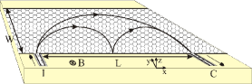
Figure 1: (Color online) Schematic geometry of the transverse electron focusing setup. A graphene nanoribbon is contacted by an injector (I) and a collector (C) probe and perpendicular (to the graphene sheet) magnetic field is applied. Classical quasiparticle trajectories leaving from the injector at normal direction, depending on the magnetic field, can be focused onto the collector.

In this paper we show that coherent electron focusing can be used in ballistic graphene samples to study the properties of the edge structure. We argue that in the case of armchair edges one would see equidistant peaks in the focusing spectrum at integer multiples of a focusing field $B_{focus}$. In contrast, for zigzag and reconstructed zigzagkoskinen (reczag) edges only the first few focusing peak would be identifiable and for stronger magnetic fields a more complex interference structure would appear in the focusing spectrum. The presence or absence of focusing peaks at stronger magnetic fields can therefore discriminate between armchair and zigzag (reczag) edges.

Our main results are summarized in Fig. 2. Using the tight-binding model for graphene with nearest-neighbour hopping we numerically calculated the transmission probability $T(B)$ from the injector to the collector as a function of the magnetic field $B$ for three different types of graphene nanoribbons: armchair, zigzag and zigzag with reconstructed edges, denoted by zz(57) in Ref. koskinen, . As Fig. 2 shows one can indeed observe peaks in the focusing spectrum of these nanoribbons. (In the one orbital per site approximation we used in the computations the focusing spectrum of the reczag nanoribbon is very similar to the simple zigzag one’s therefore we only show the latter here.) In the case of the reconstructed edge we took into account that the hopping between the atoms is different on the heptagons and pentagons than in the bulk of the graphene. To obtain realistic nearest-neighbour hoppings we employed ab-initio calculations. (See Section IV for the details of the ab-initio method and Ref. parameters, for the actual parameters of the calculations). We consider the case where there is a finite carrier density in the sample, i.e. the Fermi energy is well above of the Dirac point (this ensures that the semiclassical approach we take in Sections II and III is justified). We will focus on the transmission peaks which can be observed for $B/B_{focus}\gtrsim 1$ because they can give local information on one of the edges (see Section II). They should also be present if e.g. a graphene flake is contacted by two probes, as long as the edge between the probes is not disordered. The first peak in the transmission for all three types of nanoribbons can be found at $B/B_{focus}\approx 1$ where $B_{focus}=\frac{2\hbar k_{F}}{eL}$ ($k_{F}$ is the Fermi wavenumber (measured from the $\boldsymbol{K}$ point) and $L$ is the distance between the injector and the collector).

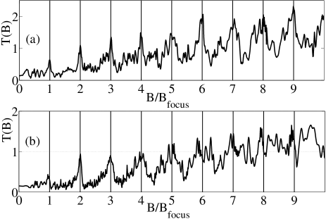
Figure 2: The results of tight binding calculations for the transmission probability $T(B)$ as a function of magnetic field. (a) for an armchair; (b) for a zigzag nanoribbon. The black vertical lines indicate the positions of the focusing peaks predicted by the semiclassical theory, see Sections II and III.

While for armchair edge there are well-defined peaks whenever $B$ is integer multiple of $B_{focus}$ [see Fig. 2(a)], in the case of zigzag edges (both the ideal and the reconstructed one) a more complex interference pattern emerges for $B/B_{focus}\gtrsim 6$ showing many oscillations but not a clear peak structure [Fig. 2(b)]. These results imply that a) one can distinguish the armchair and zigzag edges by their high magnetic field focusing spectrum; b) the difference in the focusing spectra persists even if the zigzag edge undergoes structural reconstruction. We will explain the differences in the focusing spectra of armchair and zigzag nanoribbons making use of the semiclassical theory of graphene, introduced in Refs. semi_rival, ; semi_sajat, .

The rest of the paper is organized as follows. First, in Section II we discuss the boundary conditions for the semiclassical theory on the edges of armchair and zigzag graphene nanoribbons and derive the quantization condition for edge states in magnetic field. The quantization condition then allows us to calculate the band structure. Using this in Section III we show that the focusing spectra of armchair and zigzag nanoribbons are different in strong magnetic fields. We then turn to the comparison of the results of numerical calculations and the theoretical predictions. In Section IV we discuss some details of the numerical calculations which underpin the theoretical approach presented in Sections II and III. Finally, in Section V we give our conclusions.

II Semiclassical theory of edge states in graphene

We start our discussion by establishing the link between the theory of semiclassical approximations for graphene and the boundary conditions for Dirac fermions on honeycomb lattice. If the magnetic length $l_{B}=\sqrt{\hbar/{|eB|}}$ is much larger than the lattice constant of graphene, the general energy-independent boundary condition has the form of a local restriction on the components of the wave function $\Psi$ at the edge ($\mathcal{E}$)perem_Falko ; perem_Carlo . It can be cast into the following form: $\hat{M}\Psi=\Psi$ where the $4\times 4$ matrix $\hat{M}$ may be chosen as Hermitian and unitary matrix: $\hat{M}=\hat{M}^{{\dagger}}$, and $\hat{M}^{2}=\hat{I}$. One can showperem_Carlo that demanding: a) that the probability current normal to the boundary be zero; b) that the boundary should preserve the electron-hole symmetry of the bulk; c) and finally, assuming that the boundary conditions do not break the time reversal symmetry, leads to the following form of the matrix $\hat{M}$: $\hat{M}=\big{(}\boldsymbol{\nu}\boldsymbol{\tau}\otimes\boldsymbol{n}\boldsymbol{\sigma}\big{)}$, where $\boldsymbol{\sigma}=(\sigma_{x},\sigma_{y},\sigma_{z})$, $\boldsymbol{\tau}=(\tau_{x},\tau_{y},\tau_{z})$ and $\sigma_{i}$, $\tau_{i}$ are Pauli matrices acting in the sublattice and valley space, respectively. Furthermore, $\boldsymbol{\nu}$ and $\boldsymbol{n}$ are three dimensional unit vectors, restricted to two classes: zigzag-like ($\boldsymbol{\nu}=\pm\hat{\mathbf{z}}$, $\mathbf{n}=\hat{\mathbf{z}}$, where $\hat{\mathbf{z}}$ is the unit vector perpendicular to the plane of the graphene sheet) and armchair-like ($\nu_{z}=n_{z}=0$). Additionally in both classes $\mathbf{n}\perp\mathbf{n}_{\mathcal{E}}$, where $\mathbf{n}_{\mathcal{E}}$ is a unit vector in the plane of the graphene sheet and it is perpendicular to the edge.

Let us now consider the reflection from an edge of a nanoribbon in more details. It follows from the form of the boundary conditions described earlier that the wavefunctions $\Psi^{\pm}_{\mathcal{E}}$ on the boundary is proportional to the eigenvectors $\boldsymbol{Z}^{\pm}$ corresponding to the doubly degenerate unit eigenvalue of the matrix $\hat{M}$. In other words, $\Psi^{\pm}_{\mathcal{E}}=\eta^{\pm}\boldsymbol{Z}^{\pm}e^{{\rm i}kx}$ where $\Psi^{+}$ ($\Psi^{-}$) and $\boldsymbol{Z}^{+}$ ($\boldsymbol{Z}^{-}$) correspond to isospin vector $\boldsymbol{\nu}$ (-$\boldsymbol{\nu}$), $\eta^{\pm}$ are amplitudes and $k_{x}$ is the wavevector component along the (translationally invariant) edge. On the other hand, one can show that in magnetic fields where $l_{B}\gg\lambda_{F}=2\pi/k_{F}$ ($\lambda_{F}$ is the Fermi wavelength) the wavefunctions $\Psi^{\pm}_{\mathcal{E}}$ can also be written as a superposition of an incident $\Psi_{in}$ and reflected $\Psi_{out}$ plane wave: $\Psi^{\pm}_{\mathcal{E}}=\Psi^{\pm}_{in}+\hat{r}^{\pm}\Psi^{\pm}_{out}$ where $\hat{r}^{\pm}$ are reflection amplitudes. By equating the two forms of $\Psi^{\pm}_{\mathcal{E}}$ the coefficients $\hat{r}^{\pm}$ and $\eta^{\pm}$ can be easily obtained for any boundary condition described by the matrix $\hat{M}$. For instance, in the case of armchair edge, where the isospin vector can be parametrized as $\boldsymbol{\nu}=(\cos\varphi,\sin\varphi,0)$ and $\mathbf{n}=(1,0,0)^{T}$, the eigenvectors of $\hat{M}$ with unit eigenvalues are

$$\boldsymbol{Z}^{\pm}_{a}=\frac{1}{2}\begin{pmatrix}e^{-{\rm i}\frac{\varphi}{2}}\begin{pmatrix}1\\ \pm 1\end{pmatrix}\\ e^{{\rm i}\frac{\varphi}{2}}\begin{pmatrix}\pm 1\\ 1\end{pmatrix}\end{pmatrix}.$$ (1)

The ansatz for $\Psi^{\pm}_{\mathcal{E}}$ can also be written as

$$\Psi^{\pm}_{\mathcal{E}}=\left[\frac{1}{2}\begin{pmatrix}e^{-{\rm i}\frac{\varphi}{2}}\begin{pmatrix}e^{{\rm i}\alpha}\\ 1\end{pmatrix}\\ \pm e^{{\rm i}\frac{\varphi}{2}}\begin{pmatrix}e^{{\rm i}\alpha}\\ 1\end{pmatrix}\end{pmatrix}+\frac{\hat{r}^{\pm}}{2}\begin{pmatrix}e^{-{\rm i}\frac{\varphi}{2}}\begin{pmatrix}e^{-{\rm i}\alpha}\\ 1\end{pmatrix}\\ \pm e^{{\rm i}\frac{\varphi}{2}}\begin{pmatrix}e^{-{\rm i}\alpha}\\ 1\end{pmatrix}\end{pmatrix}\right]e^{{\rm i}kx}\;$$ (2)

where $\alpha$ is the incidence angle (measured from the $x$ axis, see Fig. 1 ). Equating the two forms of $\Psi^{\pm}_{\mathcal{E}}$, i.e. $\Psi^{\pm}_{\mathcal{E}}=\eta^{\pm}\boldsymbol{Z}^{\pm}e^{{\rm i}kx}$ and Eq. (2) a straightforward calculation gives

$$\hat{r}^{\pm}_{a}=\operatorname{Exp}({\rm i}\Delta\Phi^{\pm}_{a});\quad\mbox{where}\quad\Delta\Phi^{+}_{a}=\alpha,\,\,\Delta\Phi^{-}_{a}=\alpha+\pi.$$ (3)

In the case of zigzag edges the boundary can be characterized by a superlattice vector $\boldsymbol{T}=m\boldsymbol{a}_{1}+l\boldsymbol{a}_{2}$ where $m\neq l$ are integers and $\boldsymbol{a}_{1}$, $\boldsymbol{a}_{2}$ are the lattice vectors of grapheneperem_Carlo . The boundary condition is given by $\hat{M}=\xi_{ml}\left(\tau_{z}\ \otimes\sigma_{z}\right)$ where $\xi_{ml}=\textnormal{sgn}(m-l)$, where $\textnormal{sgn}(\dots)$ is the sign function. After performing analogous calculations as for the armchair edge one finds that

$$\hat{r}^{\pm}_{z}=\operatorname{Exp}({i\Delta\Phi^{\pm}_{z}});\quad\mbox{where}\quad\Delta\Phi^{\pm}_{z}=\alpha-\pi\mp\xi_{ml}\alpha.$$ (4)

The physical meaning of Eqs. (2), (3) and (4) is the following: assuming specular reflection in classical picture the momentum of the particle is rotated upon reflection. Since the quasiparticles in graphene are chiral, the change in the direction of their momentum rotates the pseudospin as well and therefore it leads to a change in the phase of their wavefunction. As one can see from Eqs. (3) and (4) this phase shift depends on the type (armchair v. zigzag) of the edge as well. This will be important when we use semiclassical quantization to obtain the band structure of graphene armchair and zigzag nanoribbons.

A second ingredient in the calculation of the edge states is the semiclassical theory introduced in Refs. semi_rival, ; semi_sajat, . As it has been shownsemi_rival ; semi_sajat Refs. semi_rival, ; semi_sajat, , one can introduce a classical Hamiltonian $\mathcal{H}_{e}(\mathbf{p},\mathbf{r})=v_{F}\sqrt{\left(\mathbf{p}-e\mathbf{A}\right)^{2}}+V(\mathbf{r})$ for graphene to describe the classical motion of electron-like quasiparticles. Here $\mathbf{p}=(p_{x},p_{y})$ is the canonical momentum, $\mathbf{A}(\mathbf{r})$ is the vector potential describing any external magnetic field and $V(\mathbf{r})$ is scalar potential which is taken to be zero throughout our discussion, $V(\mathbf{r})=0$. If the edges of the graphene ribbon do not break the translational invariance the system is integrable because the longitudinal momentum $p_{x}$ and the energy are conserved (see Fig. 1 for the choice of the coordinate system). Using the Landau gauge $\mathbf{A}(y)=(By,0,0)^{T}$ for the vector potential to describe perpendicular magnetic field pointing into the $-\hat{z}$ direction, the Hamiltonian $\mathcal{H}_{e}$ will not depend on the $x$ coordinate and the only nontrivial quantization condition is related to the motion perpendicular to the graphene edges (in the $\hat{y}$ direction). In general it can be written as

$$\frac{1}{\hbar}S_{y}+\gamma+\Delta\Phi_{\mathcal{E}}^{\pm}=2\pi\left(n^{\pm}+\frac{\mu}{4}\right)\;,$$ (5)

where $S_{y}=\oint p_{y}\,dy$ is the classical action and the integration is over one period of the motion perpendicular to the edges. Furthermore, $\Delta\Phi_{\mathcal{E}}^{\pm}$ are the phase shifts coming from the reflections at the edges; $n^{\pm}$ is a positive integer, $\mu$ is the Maslov index counting the number of caustic points and finally $\gamma$ is a Berry-phase-like quantity semi_rival ; semi_sajat which can be calculated from the equation $\frac{{\rm d}}{{\rm d}t}\gamma\left(\mathbf{r}(t)\right)=\frac{1}{2}\left(\nabla_{\mathbf{r}}\times\frac{{\rm d}}{{\rm d}t}\mathbf{r}\right)_{z}$. Here the classical trajectory $\mathbf{r}(t)$ of quasiparticles is given bysemi_rival ; semi_sajat $\frac{{\rm d}}{{\rm d}t}\mathbf{r}=\nabla_{\mathbf{p}}\mathcal{H}_{e}(\mathbf{p},\mathbf{r})$. One can show that in perpendicular magnetic field $\gamma(\mathbf{r})$ is half of the deflection angle of the momentum of the quasiparticles.

In Landau gauge the classical action $S_{y}$ can be calculated in the same way as in Ref.semi_sajat, . The detailed presentation of the semiclassical quantization of armchair and zigzag nanoribbons in perpendicular magnetic field, discussing all the possible classical orbits and the corresponding $\gamma$ and $\Delta\Phi_{\mathcal{E}}^{\pm}$ phases is left for a forthcoming publication. For our purposes it will be sufficient to consider only those classical orbits which correspond to skipping motion along the boundaries, see e.g. in Fig.1. If the magnetic field is strong enough such that the diameter of the cyclotron orbit is smaller than the width of the nanoribbon (denoted by $W$ in Fig.1), i.e. for $2R_{c}<W$ where $R_{c}=\frac{E_{F}l_{B}^{2}}{\hbar v_{F}}$ is the cyclotron radius at Fermi energy $E_{F}$, one can show that only these skipping orbits correspond to current-carrying states. The phase shift $\Delta\Phi^{\pm}_{\mathcal{E}}$ coming from the reflection at the edge is given by Eq. (3) and Eq. (4) for armchair and zigzag edges, respectively. Considering first armchair nanoribbons, using Eqs. (3) and  (5) the semiclassical quantization of skipping orbits reads

$$k_{F}R_{c}\left(\frac{\pi}{2}+\beta_{n}^{\pm}+\frac{1}{2}\sin 2\beta_{n}^{\pm}\right)=2\pi\left(n^{\pm}\pm\frac{1}{4}\right)$$ (6)

where $k_{F}=\frac{E_{F}}{\hbar v_{F}}$, $\beta_{n}^{\pm}$ is the angle with the $y$ axis under which the cyclotron orbit is reflected from the boundary, and $+$($-$) corresponds to isospin $\boldsymbol{\nu}$($-\boldsymbol{\nu}$). Moreover, $n^{+}=0\dots n_{max}^{+}$ ($n^{-}=1\dots n_{max}^{-}$) where $n_{max}^{\pm}$ is the largest integer smaller than $\frac{1}{2}k_{F}R_{c}\mp\frac{1}{4}$. This quantization conditions holds for both metallic and insulating armchair nanoribbons. The physical meaning of Eq. (6) is that the enclosed flux by the cyclotron orbit and the edge of the nanoribbon is quantized and it must equal $h/e(n^{\pm}\pm 1/4)$. It is interesting to note that for 2DEG with hard wall boundary conditions the quantization condition for edge states looks very similar, except that one would have to omit the $\pm$ sign and on the right hand side one would have $(n+\frac{3}{4})$.

The semiclassical quantization for edge states in the case of zigzag nanoribbon can be obtained in the same way as for an armchair nanoribbon, the only difference is that instead of Eq. (3) one has to use Eq. (4). One finds that it is given by

$$\begin{split}k_{F}R_{c}\left(\frac{\pi}{2}+\beta_{n}^{\pm}+\frac{1}{2}\sin 2\beta_{n}^{\pm}\right)-&\nu\xi_{ml}\left(\frac{\pi}{2}+\beta_{n}^{\pm}\right)\\ =&\,\,2\pi\left(n^{\pm}-\frac{1}{4}\right).\end{split}$$ (7)

Here $\pm$ corresponds to the product $\nu\xi_{ml}=\pm 1$, where both $\nu$ and $\xi_{ml}$ can take on values $\pm 1$. The value of $\nu$ depends on the isospin: it is $1$ ($-1$) if the isospin is $\boldsymbol{\nu}=\hat{z}$ ($\boldsymbol{\nu}=-\hat{z}$) and $\xi_{ml}=\pm 1$ is introduced before Eq. (4). The range of the quantum number $n^{\pm}$ is the same as for the armchair case. One can notice that as compared to Eq. (6) there is an extra term on the left hand side of Eq. (7). The origin of the difference in the focusing spectra of armchair and zigzag nanoribbons, to be discussed in Section III, can be traced back to this term in the dispersion relation.

We have calculated the band structure for armchair and zigzag nanoribbons in homogeneous perpendicular magnetic field both semiclassically, using Eqs. (6), (7), and numerically in tight binding approximation.

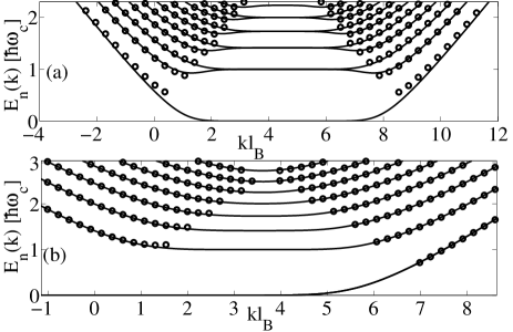
Figure 3: Comparison of the results for the band structure obtained from semiclassical quantization given by Eqs. (6),  (7) (circles) and from numerical tight binding calculations (solid lines). The energy is in units of $\hbar\omega_{c}=\sqrt{2}\frac{\hbar v_{F}}{l_{B}}$. The magnetic field is given by $W/l_{B}=8.97$. (a) armchair nanoribbon; (b) zigzag nanoribbon, in the vicinity of the $\boldsymbol{K}$ point.

As one can see in Fig. 3 the agreement between the semiclassical and the tight-binding calculations is very good except for low energies $E/\hbar\omega_{c}\lesssim 1/2$. (The dispersionless state of a zigzag nanoribbon at zero energy cannot be described by semiclassics either.) However, the dispersionless sections of the band structure corresponding to Landau levels at finite energies can be calculated semiclassicallysemi_rival ; semi_sajat . (We note that similar results have been obtained in Ref. gusynin, using the Dirac-like Hamiltonian for graphene.)

III Magnetic focusing in graphene nanoribbons

Having obtained the quantization condition for edge states in Eqs. (6) and  (7), the calculation of the magnetic fields $B_{focus}$, where the transmission between the injector and collector is sharply peaked, follows the reasoning of Ref. Houten_Carlo1:cikk, . The ballistic transport along the edges of a nanoribbon can be understood in terms of the edge states described in Section II because they are the propagating modes of this problem. If the injector is narrow ($\sim\lambda_{F}$) one can assume that it excites these modes coherently. Therefore, as long as the distance between the injector and the collector is smaller than the phase coherence length, the interference of the edge states can be important. For a given $E_{F}$ the interference of the edge states, labelled by $n^{\pm}$ in Eqs. (6) and (7), is determined by the phase factors $\exp(ik_{n}^{\pm}L)$. Here the wave numbers $k_{n}^{\pm}$ are given by $k_{n}^{\pm}=k_{F}\sin\beta_{n}^{\pm}$ and $L$ is the distance between the (very narrow) injector and collector. Both in the armchair and in the zigzag case one can show that around $n^{\pm}=n_{max}^{\pm}/2$, which corresponds to $|\beta_{n}^{\pm}|\ll 1$, in good approximation the angles $\beta_{n}^{\pm}$ depend linearly on $n^{\pm}$.

Expanding Eq. (6) around $\beta_{n}^{\pm}=0$ one finds that

$$k_{n}^{\pm}L\approx\frac{\pi L}{R_{c}}\left(n^{\pm}\pm\frac{1}{4}\right)-C_{a}+\frac{k_{F}L}{3}\left(\frac{\pi}{4}\frac{n_{max}^{\pm}-2n^{\pm}}{n_{max}^{\pm}}\right)^{3}$$ (8)

where $C_{a}=\frac{\pi}{4}k_{F}L$. This result means that if $L/2R_{c}$ is an integer (or equivalently, $B/B_{focus}$ is integer, where $B_{focus}=\frac{2\hbar k_{F}}{eL}$) some edge channels, with quantum numbers $n^{\pm}$ centred around $n_{max}^{\pm}/2$, can constructively interfere at the collector. Other edge states, to which the linear expansion shown in Eq. (8) cannot be applied, give rise to an additional interference pattern which does not have a simple periodicity. The expression for the focusing field $B_{focus}$ is formally the same as for 2DEGHouten_Carlo1:cikk but the dependence of $k_{F}$ on the electron density is different in the two systems.

Repeating the expansion for zigzag nanoribbons using Eq. (7) we find that to linear order

$$k_{n}^{\pm}L\approx\frac{1}{1\mp\frac{1}{4\kappa^{2}}}\frac{\pi L}{R_{c}}\left(n^{\pm}+\frac{1}{4}\pm\frac{1}{4}\right)-C_{z}\\$$ (9)

where $\kappa=E_{F}/\hbar\omega_{c}$ is the filling factor and $C_{z}=-\frac{\pi}{4}k_{F}L\frac{1}{1\mp\frac{1}{4\kappa^{2}}}$. For nanoribbons where the cyclotron radius becomes smaller than the width of the ribbon such that $\kappa\gg 1$ is satisfied and therefore $1/\left(1\mp\frac{1}{4\kappa^{2}}\right)\approx 1$ the focusing field $B_{focus}$ can be defined in the same way as for armchair ribbons and the transmission peaks are at the same focusing fields as in the armchair case. However, according to Eq. (9) as $\kappa$ gets smaller for increasing magnetic field (assuming fixed Fermi energy) the focusing field for the two isospin index becomes slightly different, moreover, the subsequent focusing fields for each isospin index are no longer equidistant. (Examination of the higher order terms not shown in Eq. (9) reveals that also the number of interfering edge channels becomes different for the two isospin indices.) As a result, a more complex interference pattern is expected to appear than in the case of armchair nanoribbon and a simple $B_{focus}$ can no longer be defined.

Turning to the comparison of the numerical results shown in Fig. 2 with the analytical predictions given in Eqs. (8) and (9), one should focus on the $B/B_{focus}\geq 1$ regime, where the edge states are the current carrying modes. One can see that the peak positions for the armchair nanoribbon are in very good agreement with the prediction of the semiclassical theory. Up to $B/B_{focus}\lesssim 5$ the focusing peaks are also clearly discernible in the focusing spectra of zigzag nanoribbons but for stronger magnetic fields a more complex interference pattern emerges. The peak at $B/B_{focus}=7$ for example can clearly be seen for the armchair case. In contrast, for the zigzag edge a number of oscillations with similar amplitudes can only be observed. The difference between focusing spectra of the armchair on one hand and of the zigzag (and reczag) edges on the other hand is even more noticeable in stronger magnetic fields, i.e. for $B/B_{focus}>7$. (Eventually, at very strong magnetic fields the cyclotron radius of the quasiparticles would become comparable to the width of the collector and the system would therefore be equivalent to a Hall bar. We will not consider this regime here.) Note, that for a typical electron density of $n_{e}=2.5\times 10^{16}\frac{1}{m^{2}}$ and assuming $L=1\mu m$ the focusing field is $B_{focus}\approx 0.37T$, which is experimentally feasible.

In the case of the calculations presented in Fig. 2 the width $W$ of the nanoribbon was larger than $L/2$ ($L$ is the injector-collector distance). This meant that for the Fermi energy we used already the $p=1$ focusing peak could be observed. For narrow ribbons however it can easily happen that for given $E_{F}$ and $W$ the first few peaks would not appear, until for sufficiently strong field the cyclotron radius $R_{c}$ becomes smaller than $W$ and the condition $2*p*R_{c}=L$ is met for some integer $p$. For narrow zigzag and reczag ribbons therefore there might be no observable focusing peaks because for the magnetic fields where $R_{c}$ would become small enough, the $\kappa\gg 1$ condition [see below Eq. (9)] is no longer satisfied. There could be of course oscillations or peaks in the transmission even in this case but those would not have the simple periodicity that focusing peaks have.

IV Details of the numerical calculations

Let us now briefly discuss some of the details of our numerical calculations for the transmission probability $T(B)$ shown in Fig. 2. The injector and the collector were modeled by heavily doped graphene and the transmission was calculated employing the Green’s function technique of Ref. sanvito, . The graphene nanoribbons are assumed to be perfectly ballistic and infinitely long. This means that the left and right ends of the nanoribbons act as drains which absorb any particles exiting to the left of right. To simulate the effect of finite temperatures we used a simple energy averaging procedure in the calculation of the transmission curves: $T(B)=\int T(B,E)\left(-\frac{\partial f_{0}(E)}{\partial E}\right)dE$ where $f_{0}(E)$ is the Fermi function. The actual results shown in Fig. 2 were calculated at $T=1K$ temperature. As it can be expected, higher temperatures tend to smear the curves while at lower ones an additional fine structure appears.

For simple armchair and zigzag nanoribbons we assumed that the hopping parameter between the atoms is the same everywhere on the ribbons. In contrast, for the zz(57) edge we took into account that the hopping parameter changes on the pentagons and heptagons at the edges with respect to its the bulk value.

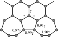
Figure 4: The reconstructed zigzag edge. The numbers indicate the change of the hopping parameter on particular bonds with respect to its bulk value, $\gamma=-3.39eV$.

We calculated the hoppings with density-functional tight-binding (DFTB) method, using the hotbit code.hotbit_wiki This approach yields the hopping matrix elements as two-center integrals for pseudo-atomic orbitals that result from a straightforward pathway of ab initio calculations, as described in Ref. koskinen_CMS_09, . The density-functional parametrization yields a valid description of the covalent bonding in carbon nanomaterials.frauenheim_JPCM_02 Fig.4 shows the relative hoppings from DFTB-optimized geometry, note how the appearance of a triple bond in the armrest parts affects also the $\pi$-electron hopping, due to the significant reduction in bond length.koskinen

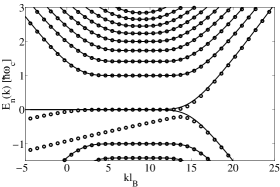
Figure 5: Comparison of the band structures of zigzag (solid line) and reczag (circles) nanoribbons from tight binding calculations at the K point. The strength of the magnetic field is given by $W/l_{B}=9.14$.

In the one orbital per site approximation we employed here the band structures of zigzag and reczag nanoribbons, apart from the close vicinity of the Dirac point, are very similar (see Fig. 5). This explains why they have very similar focusing spectra as well.

V Summary

In summary, we studied coherent electron focusing in graphene nanoribbons using both exact quantum calculations and in semiclassical approximation. We found that in the case of armchair edges the transmission peaks are at integer multiples of $B/B_{focus}$ whereas for zigzag edges such a simple rule holds only when the filling factor $\kappa$ is much larger than unity. For zigzag nanoribbons in stronger magnetic field, when the filling factor is of the order of one, a more complex interference pattern can be observed in the transmission and the emergence of this interference pattern can be understood from semiclassical calculations. The presence of focusing peaks at low magnetic fields can therefore attest to the quality of the edge structure, while measurements at stronger fields can discriminate between armchair and zigzag edges. Our numerical calculations on zz(57) edges suggest that the above conclusion holds even if the zigzag edge is structurally reconstructed. Although we considered in our analytical calculations nanoribbons whose both edges had perfect armchair or zigzag structure, we expect that our findings are more generally valid. Namely, they rely on the properties of edges states localized at one of the edges therefore imperfections of the other edge should not affect the focusing peaks. Therefore this technique should be applicable to study the edges of graphene flakes as well. Finally, an interesting extension of our work would be to consider the focusing spectrum of other proposedwassmann edge types and possibly taking into account more than one orbital per site in the transport computations.

References

- (1) V. S. Tsoi, J. Bass, and P. Wyder, Rev. Mod. Phys. 71, 1641 (1999).
- (2) H. van Houten, C. W. J. Beenakker, J. G. Williamson, M. E. I. Broekaart, P. H. M. van Loosdrecht, B. J. van Wees, J. E. Mooij, C. T. Foxon, and J. J. Harris, Phys.Rev. B 39, 8556 (1989).
- (3) K. S. Novoselov, A. K. Geim, S. V. Morozov, D. Jiang, Y. Zhang, S. V. Dubonos, I. V. Grigorieva, and A. A. Firsov, Science 306, 666 (2004).
- (4) L. Tapasztó, G. Dobrik, P. Lambin, L. P. Biró, Nature Nanotechnology 3, 397 (2008).
- (5) M. Y. Han, B. Özyilmaz, Y. Zhang and Ph. Kim, Phys. Rev. Lett 98, 206805 (2007).
- (6) Xiaoting Jia, M. Hofmann, V. Meunier, B. G. Sumpter, J. Campos-Delgado, J. M. Romo-Herrera, H. Son, Ya-Ping Hsieh, A. Reina, J. Kong, M. Terrones, and M. S. Dresselhaus, Science 323, 1701 (2009).
- (7) Çağlar Ö Girit J. C. Meyer, R. Erni, M. D. Rossell, C. Kisielowski, Li Yang, Cheol-Hwan Park, M. F. Crommie, M. L. Cohen, S. G. Louie, and A. Zettl, Science 323, 1705 (2009).
- (8) K. A. Ritter and J. W. Lyding, Nature Materials 8, 235 (2009).
- (9) K. Wakabayashi, M. Fujita, H. Ajiki, and M. Sigrist, Phys. Rev. B 59, 8271 (1999).
- (10) K. Wakabayashi, Y. Takane, M. Yamamoto, and M. Sigrist, New J. Phys. 11, 095016 (2009).
- (11) Y.-W. Son, M. L. Cohen and S. G. Louie, Phys. Rev. Lett 97, 216803 (2006).
- (12) L. Pisani, J. A. Chan, B. Montanari, and N. M. Harrison, Phys. Rev. B 75, 064418 (2007).
- (13) P. Koskinen, S. Malola, H. Häkkinen, Phys. Rev. Lett 101, 115502 (2008).
- (14) P. Koskinen, S. Malola, H. Häkkinen, Phys. Rev. B 80, 073401 (2009).
- (15) T. Wassmann, A. P. Seitsonen, A. M. Saitta, M. Lazzeri, and F. Mauri Phys. Rev. Lett 101, 096402 (2008).
- (16) For the calculations shown in Fig.2 we considered graphene nanoribbons for which and . The width of the injector and collector probes were and we assumed that the electron density in the ribbon was . Although the limitations of our numerics did not allow us to consider experimentally more realistic cases (i.e. and ) we are confident that our main results are robust and can therefore have experimental relevance.
- (17) S. Sanvito, C. J. Lambert, J. H. Jefferson and A. M. Bratkovsky, Phys. Rev. B 59, 11936 (1999).
- (18) E. McCann and V. I. Fal’ko, J. Phys. Condens. Matter 16, 2371 (2004).
- (19) A. R. Akhmerov, C. W. J. Beenakker, Phys. Rev. B 77, 085423 (2008).
- (20) P. Carmier and D. Ullmo, Phys. Rev. B 77, 245413 (2008).
- (21) A. Kormányos, P. Rakyta, L. Oroszlány, J. Cserti, Phys. Rev. B 78, 045430 (2008).
- (22) V. P. Gusynin, V. A. Miransky, S. G. Sharapov, I. A. Shovkovy, and C. M. Wyenberg, Phys. Rev. B 79, 115431 (2009).
- (23) P. Koskinen and V. Mäkinen, Comput. Mat. Sci. 47, 237 (2009).
- (24) hotbit wiki at https://trac.cc.jyu.fi/projects/hotbit
- (25) T. Frauenheim, G. Seifert, M. Elstner, T. Niehaus, C. Köhler, M. Amkreutz, M. Sternbergand, Z. Hajnal, A. Di Carlo, and S. Suhai J. Phys.: Condens. Matter. 14, 3015 (2002).