Influence of Ohmic diffusion on the excitation and dynamics of MRI

Abstract

In this paper we make an effort to understand the interaction of turbulence generated by the magnetorotational instability (MRI) with turbulence from other sources, such as supernova explosions (SNe) in galactic disks. First we perform a linear stability analysis (LSA) of non-ideal MRI to derive the limiting value of Ohmic diffusion that is needed to inhibit the growth of the instability for different types of rotation laws. With the help of a simple analytical expression derived under first-order smoothing approximation (FOSA), an estimate of the limiting turbulence level and hence the turbulent diffusion needed to damp the MRI is derived. Secondly, we perform numerical simulations in local cubes of isothermal nonstratified gas with external forcing of varying strength to see whether the linear result holds for more complex systems. Purely hydrodynamic calculations with forcing, rotation and shear are made for reference purposes, and as expected, non-zero Reynolds stresses are found. In the magnetohydrodynamic calculations, therefore, the total stresses generated are a sum of the forcing and MRI contributions. To separate these contributions, we perform reference runs with MRI-stable shear profiles (angular velocity increasing outwards), which suggest that the MRI-generated stresses indeed become strongly suppressed as function of the forcing. The Maxwell to Reynolds stress ratio is observed to decrease by an order of magnitude as the turbulence level due to external forcing exceeds the predicted limiting value, which we interpret as a sign of MRI suppression. Finally, we apply these results to estimate the limiting radius inside of which the SN activity can suppress the MRI, arriving at a value of 14 kpc.

1 Introduction

Most differentially rotating astrophysical disks are susceptible to the magnetorotational instability (MRI). In accretion disks this instability is likely to be the most important source of turbulence and angular momentum transport leading to mass accretion (originally proposed by Balbus & Hawley 1991). It has also been proposed that the MRI would play a role in driving turbulence in the outer parts of galactic disks where the stellar forcing is of minor importance (Sellwood & Balbus 1999; see also Piontek & Ostriker 2007 and references therein).

Whether the powerful stellar forcing suppresses or interacts with the galactic MRI in the inner parts of galactic disks is still an open question. The study by Workman & Armitage (2008), who investigated the interaction of the MRI with nonhelically forced turbulence in isothermal nonstratified local cubes of gas with Keplerian differential rotation, can be regarded as a first step to understand this issue. They found that external turbulence can indeed modify the turbulent transport when the level of turbulence becomes greater than the strength of the MRI-generated turbulence, and that the degree of the influence is dependent on the forcing scale. Only turbulence forced at large wavenumbers (smallest scales) was interpreted to suppress MRI, while large-scale forcing seemed to enhance it. In this study we show that the forcing wavenumber dependence can be understood with the help of the linear stability analysis. We also show that reference calculations with MRI-stable rotation profiles are needed to fully determine the level of turbulence and angular momentum transport that results from the MRI in comparison to other sources of turbulence.

The paper is organised as follows. In Sect. 2 we present a linear stability analysis of non-ideal MRI to derive the limiting value of Ohmic diffusion that is needed to inhibit the growth of the instability for different types of rotation laws. We also present an estimate of the level of turbulence needed to produce turbulent Ohmic diffusion strong enough to suppress MRI in the isotropic homogeneous case using the first-order smoothing approximation (hereafter FOSA). In Sect. 3, we introduce the model that we use to study the dynamics of the MRI under the influence of external nonhelical forcing. First we apply this model to carry out simple one-dimensional calculations to reproduce the linear results of Sect. 2 and then to three-dimensional hydro- and magnetohydrodynamic models of isothermal, nonstratified, rotating and shearing cubic domains subject to rotation laws both unstable and stable with respect to the MRI. The latter have been used to calibrate the former to get a better understanding of turbulence resulting from the MRI with respect to the turbulence resulting from the interaction of external forcing, rotation and shear. The results of these calculations are presented in Sect. 4. In Sect. 5 we present a simple application of our results to galactic disks. In Sect. 6 we present our conclusions.

2 Linear stability analysis of non-ideal MRI

Jin (1996) presented linear stability analysis of non-ideal MRI for disks with Keplerian rotation profiles. Here we generalise the theory to include any rotation profile of the form $\Omega\propto r^{-q}$, further assuming that the system is incompressible and pressureless.

We choose a local Cartesian frame of reference, in which $x$, $y$ and $z$ denote the radial, toroidal and vertical directions, respectively. We start by linearizing the pressureless ideal equation of motion

$$\frac{\partial\bm{U}}{\partial t}+(\bm{U}\cdot\bm{\nabla})\bm{U}+2\,\bm{\Omega}\times\bm{U}-\frac{1}{\rho}\bm{J}\times\bm{B}=0\;,$$ (1)

and the non-ideal induction equation

$$\frac{\partial\bm{B}}{\partial t}-\bm{\nabla}\times(\bm{U}\times\bm{B})=\eta\bm{\nabla}^{2}{\bm{B}}\;,$$ (2)

around the location of the centre of the box, $r_{0}$, in a differentially rotating disk that is subject to a weak uniform vertical magnetic field $B_{0}\hat{\bm{e}}_{z}$. Here $\bm{U}$ is the velocity field, $\bm{B}$ is the magnetic field, $\bm{J}=\mu_{0}^{-1}\bm{\nabla}\times\bm{B}$ is the current density, $\mu_{0}$ is the vacuum permeability, and $\eta$ is the Ohmic diffusion coefficient. The angular velocity at $r_{0}$ is $\Omega_{0}$, and it varies with the distance from the centre as $\Omega\propto r^{-q}$. Such differential rotation translates into a radially linear shearing velocity ${\bm{U}}_{0}=-q\Omega_{0}x\hat{\bm{e}}_{y}$ after the linearization of Eq. (1). Small fluctuations ${\bm{u}}=\left[u_{x},u_{y},u_{z}\right],\ {\bm{b}}=\left[b_{x},b_{y},b_{z}\right]$ are now added to the equilibrium state ${\bm{U}}_{0}=\left[0,-q\Omega_{0}x,0\right],\ {\bm{B}}_{0}=\left[0,0,B_{0}\right]$. We consider only fluctuations in the vertical ($z$) direction, as fluctuations of this type have been shown to have the highest growth rates (Balbus & Hawley 1992); in this case the equations for the $z$-components of velocity and magnetic field decouple from the horizontal ones and therefore they can be neglected. The set of linearised equations for the horizontal fluctuating fields in component form read

$$\frac{\partial u_{x}}{\partial t} = 2\,\Omega_{0}u_{y}+\frac{B_{0}}{\mu_{0}\rho}\frac{\partial b_{x}}{\partial z}\;,$$ (3)

$$\frac{\partial u_{y}}{\partial t} = -\left(2-q\right)\Omega_{0}u_{x}+\frac{B_{0}}{\mu_{0}\rho}\frac{\partial b_{y}}{\partial z}\;,$$ (4)

$$\frac{\partial b_{x}}{\partial t} = B_{0}\frac{\partial u_{x}}{\partial z}+\eta\frac{\partial^{2}b_{x}}{\partial z^{2}}\;,$$ (5)

$$\frac{\partial b_{y}}{\partial t} = -q\Omega_{0}b_{x}+B_{0}\frac{\partial u_{y}}{\partial z}+\eta\frac{\partial^{2}b_{y}}{\partial z^{2}}\;.$$ (6)

Let us now assume that the solutions to these equations are of the form $f_{j}=\hat{f}_{j}e^{i\left(kz-\omega t\right)}$. Substitution yields a set of algebraic equations

$$-i\omega\hat{u}_{x} = 2\,\Omega_{0}\hat{u}_{y}+ik\frac{B_{0}}{\mu_{0}\rho}\hat{b}_{x}\;,$$ (7)

$$-i\omega\hat{u}_{y} = -\left(2-q\right)\Omega_{0}\hat{u}_{x}+ik\frac{B_{0}}{\mu_{0}\rho}\hat{b}_{y}\;,$$ (8)

$$-i\omega\hat{b}_{x} = ikB_{0}\hat{u}_{x}-k^{2}\eta\hat{b}_{x}\;,$$ (9)

$$-i\omega\hat{b}_{y} = -q\Omega_{0}\hat{b}_{x}+ikB_{0}\hat{u}_{y}-k^{2}\eta\hat{b}_{y}\;.$$ (10)

From these equations the following dispersion relation is obtained:

$$\omega^{4} + 2i\Omega_{m}\omega^{3}$$ (11)

$$- \left(2\left(2-q\right)\Omega_{0}^{2}+\Omega_{\rm m}^{2}+2k^{2}v_{\rm A}^{2}\right)\omega^{2}$$

$$- i\Omega_{m}\left(4\left(2-q\right)\Omega_{0}^{2}+2k^{2}v_{\rm A}^{2}\right)\omega$$

$$+ \!k^{2}v_{\rm A}^{2}(k^{2}v_{\rm A}^{2}\!-\!2q\Omega_{0}^{2})\!+\!2\left(2-q\right)\Omega_{0}^{2}\Omega_{\rm m}^{2}\!=\!0,$$

where $v^{2}_{\rm A}=\frac{B_{0}^{2}}{\mu_{0}\rho}$, and $\Omega_{\rm m}=\eta k^{2}$. We have numerically solved the dispersion relation searching especially for the limiting Ohmic diffusion rate at which all the MRI modes become damped. In practise we solve for all the four roots of the dispersion relation and require that all the imaginary parts are negative. The results of this analysis are plotted in Figs. 1 and 2.

In Fig. 1 we show all imaginary parts of the four roots of the dispersion relation for $q=1.5$, $k_{\rm max}/k=1$, where $k_{\rm max}=\frac{q}{2}\frac{v_{\rm A}}{\Omega_{0}}\sqrt{\frac{4}{q}-1}$, as functions of the Ohmic diffusion rate $\Omega_{\rm m}$. We have scaled $\Omega_{\rm m}$ with the maximum growth rate, $\Gamma_{\rm max}$, of the ideal MRI. From these results it can be seen that in the ideal limit $\Omega_{\rm m}=0$ the growth rate of the MRI mode is positive and equal to $\Gamma_{\rm max}=\frac{q}{2}\Omega_{0}$. As the diffusion is increased, the growth rate decreases and reaches zero at $\Omega_{\rm m}\approx 1.9\Gamma_{\rm max}$. As the growth rates of the other modes are negative for all values of $\Omega_{\rm m}$, then this is the limiting diffusion rate above which the instability will be damped for $k=k_{\rm max}$. Our results are in agreement with those of Jin (1996); due to the incompressibility assumption the inertial wave mode is absent in our analysis, but the limiting Ohmic diffusion rate for MRI damping is identical for the Keplerian case in both studies.

In Fig. 2 we have determined the limiting Ohmic diffusion rate for each value of $q,\ 0<q<2$, where the system is ideally unstable, for all values of $k=[0,k_{\rm crit}]$, where $k_{\rm crit}=\frac{\Omega_{0}}{v_{\rm A}}\sqrt{2q}$ is the largest MRI-unstable ideal wavenumber. Analytical ‘stability criterion’ can also be derived from the analysis: MRI will be damped if

$$\Omega_{\rm m}>\frac{kv_{\rm A}}{\Omega_{0}}\sqrt{\frac{2q\Omega_{0}^{2}-k^{2}v_{\rm A}^{2}}{2\left(2-q\right)}}.$$ (12)

At the limit $q=2$, the Ohmic diffusion rate becomes infinite, meaning that in this regime the flow cannot be stabilized by the Ohmic diffusion. We find that for small $q$ the results for the maximally excited and all unstable wavenumbers are identical, whereas for larger $q$ they start to deviate more and more indicating that some wavenumbers are harder to damp than the one with the largest growth rate. From this plot we can also see that for very small $q$ the limiting value approaches the maximum growth rate, $\Gamma_{\rm max}$, of the ideal MRI. The limiting Ohmic diffusion rate increases with $q$ above $\Gamma_{\rm max}$ so that for rotation profiles near the Rayleigh unstable regime ($q>2$) the Ohmic diffusion rate needed to damp the MRI is roughly three times $\Gamma_{\rm max}$.

2.1 FOSA-prediction for isotropic homogeneous turbulence

Let us now use the information obtained from the linear stability analysis to make a prediction for the nonlinear setup we use in the rest of the paper. Firstly we need an estimate of the turbulent Ohmic diffusion resulting from the isotropic external forcing at a wavenumber $k_{\rm f}$. In order to obtain this we can use the first-order smoothing approximation (FOSA) result

$$\eta_{\rm t}={\textstyle{1\over 3}}\tau_{c}u_{\rm rms}^{2}={\textstyle{1\over 3}}u_{\rm rms}k_{\rm f}^{-1},$$ (13)

where we have assumed that the Strouhal number, ${\rm St}=\tau_{c}u_{\rm rms}k_{\rm f}$, is equal to unity. This value has been confirmed in the kinematic regime numerically by Sur et al. (2008) from non-shearing setups using the test field method (Schrinner et al. 2005, 2007). In the presence of shear the value of $\eta_{\rm t}$ can increase slightly but is still of the same order of magnitude (Brandenburg et al. 2008; Mitra et al. 2009). Therefore we obtain

$$\Omega_{\rm m}=\eta_{\rm t}k_{\rm f}^{2}={\textstyle{1\over 3}}u_{\rm rms}k_{\rm f},$$ (14)

for the turbulent Ohmic diffusion rate. From the linear stability analysis we know that MRI will be damped if

$$\Omega_{\rm m}>A(q)\Gamma_{\rm max}=\frac{qA(q)}{2}\Omega_{0},$$ (15)

where $A(q)$ varies from 1 to roughly 3 as $q$ is increased from 0 to 2 (see Fig. 2). By substituting the FOSA-expression, Eq. (13), we can simplify this further, yielding the condition

$$u_{\rm rms}>\frac{3qA(q)\Omega}{2k_{\rm f}},$$ (16)

for the suppression of MRI. Note that for a given $u_{\rm rms}$ this condition is dependent on the spatial scale of the turbulence so that the larger the scale, the harder it is to damp MRI.

Figure 1: Imaginary parts of the roots of the non-ideal dispersion relation for the Keplerian case $q=1.5$ as function of the Ohmic diffusion rate scaled with the maximum growth rate $\Gamma_{\rm max}$ of the MRI. Solid thick line represents the (fast) MRI mode, dashed line the decay mode, and the dotted line the slow mode (given by two roots with equal imaginary parts). The dashed-dotted line indicates $\omega_{i}/\Omega_{0}$=0.

Figure 2: Limiting Ohmic diffusion rate $\Omega_{\rm m}$ at which MRI modes corresponding to the range of wavenumbers $k=[0,k_{\rm crit}]$ (solid line with diamonds) and for a single wavenumber $k=k_{\rm max}$ (dashed line with triangles) are damped as functions of $q$. The results are scaled with the maximum growth rate of the ideal MRI, $\Gamma_{\rm max}$. The dotted line shows the limit at which the Ohmic diffusion rate and maximum growth rate of MRI are equal for reference.

3 Model

We use a model setup similar to that used in Liljeström et al. (2009), except that here we add an external forcing function in the Navier–Stokes equation. The computational domain is a cube of size $(2\pi)^{3}$, filled with isothermal gas; vertical gravity and stratification are neglected. The calculations are local and utilise the shearing-sheet approximation. The equations to be solved read

$$\frac{\mathcal{D}\rho}{\mathcal{D}t} = -\bm{\nabla}\cdot(\rho\bm{u})\;,$$ (17)

$$\frac{\mathcal{D}\bm{u}}{\mathcal{D}t} = -(\bm{u}\cdot\bm{\nabla})\bm{u}-q\Omega_{0}u_{x}\hat{\bm{e}}_{y}-2\,\Omega_{0}\hat{\bm{e}}_{z}\times\bm{u}$$ (18)

$$-\frac{1}{\rho}\bm{\nabla}p+\frac{1}{\rho}\bm{J}\times\bm{B}+\nu_{\rm h}\nabla^{6}\bm{u}+f_{\rm force},$$

$$\frac{\mathcal{D}\bm{A}}{\mathcal{D}t} = \bm{u}\times\bm{B}+q\Omega_{0}A_{y}\hat{\bm{e}}_{x}+\eta_{\rm h}\nabla^{6}\bm{A}\;,$$ (19)

where $\mathcal{D}/\mathcal{D}t=\partial/\partial t+U_{0}\partial/\partial y$ includes advection by the shear flow, $\bm{u}$ is the departure from the mean flow $\bm{U}_{0}$, $\rho$ is the density, $p$ is the pressure, $\bm{A}$ is the magnetic vector potential, $\bm{B}=\bm{\nabla}\times{\bm{A}}$ is the magnetic field, and ${\bm{J}}=\bm{\nabla}\times{\bm{B}}/\mu_{0}$ is the current density. In order to get as close as possible to the ideal limit, we use hyperviscous operators of the form $\nabla^{6}$ to replace the ordinary viscosity $\nabla^{2}$-operators; $\nu_{\rm h}$ and $\eta_{\rm h}$ stand for the hyperviscous kinematic viscosity and magnetic diffusivity, respectively. With this procedure we aim at maximizing the Reynolds number in the quiescent regions of the flow while diffusing and damping fluctuations near the grid scale. Compared to direct simulations (e.g. Haugen & Brandenburg 2006) with uniform viscosities, smaller grid size can be used to resolve the flow.

The forcing function $\bm{f}_{\rm force}$ is given by

$$\bm{f}(\bm{x},t)={\rm Re}\{N\bm{f}_{\bm{k}(t)}\exp[i\bm{k}(t)\cdot\bm{x}-i\phi(t)]\}\;,$$ (20)

where $\bm{x}$ is the position vector, $N=f_{0}c_{\rm s}(kc_{\rm s}/\delta t)^{1/2}$ is a normalization factor, $f_{0}$ is the forcing amplitude, $k=|\bm{k}|$, $\delta t$ is the length of the time step, and $-\pi<\phi(t)<\pi$ a random delta-correlated phase. The vector $\bm{f}_{\bm{k}}$ is given by

$$\bm{f}_{\bm{k}}=\frac{\bm{k}\times\hat{\bm{e}}}{\sqrt{\bm{k}^{2}-(\bm{k}\cdot\hat{\bm{e}})^{2}}}\;,$$ (21)

where $\hat{\bm{e}}$ is an arbitrary unit vector. Thus, $\bm{f}_{\bm{k}}$ describes nonhelical transversal waves with $|\bm{f}_{\bm{k}}|^{2}=1$, where ${\bm{k}}$ is chosen randomly from a predefined range in the vicinity of the average nondimensional wavenumber $k_{\rm f}/k_{1}$ at each time step. Here $k_{1}$ is the wavenumber corresponding to the domain size, and $k_{\rm f}$ is the wavenumber of the energy-carrying scale.

Periodic boundary conditions are applied in all three directions; in the radial direction we account for the shear flow $\bm{U}_{0}$ by making use of the shearing-sheet approximation (e.g. Wisdom & Tremaine 1988):

$$f({\textstyle{1\over 2}}L_{x},y,z)=f(-{\textstyle{1\over 2}}L_{x},y+q\Omega_{0}L_{x}t,z),$$ (22)

where $f$ stands for any of the seven independent variables, $L_{x}$ for the radial extent of the computational domain, and $t$ is the time.

The domain is initially threaded by a weak magnetic field,

$${\bm{A}}=A_{0}\hat{\bm{e}}_{y}\cos k_{\rm A}x\cos k_{\rm A}y\cos k_{\rm A}z\;.$$ (23)

Thus, the magnetic field contains periodic $x$- and $z$-components with amplitude $A_{0}$. The values of $k_{\rm A}$, $\Omega_{0}$ and $A_{0}$ are selected so that both the wavenumber with the largest growth rate, $k_{\rm max}$, and the largest unstable wavenumber, $k_{\rm crit}$, are well resolved by the grid; in practise this means that in the three-dimensional calculations we adopt $k_{\rm A}/k_{1}=1$, $\Omega_{0}=0.2c_{\rm s}k_{1}$ and $A_{0}=0.2\sqrt{\mu_{0}\rho_{0}}\,c_{\rm s}k_{1}^{-1}$, resulting in $k_{\rm max}=O(k_{1})$. For the initial setup, the other condition for the onset of MRI, namely $\beta\gg 1$, where $\beta=2\mu_{0}p/B_{0}^{2}$ is the ratio of the thermal to magnetic pressure, is also satisfied as $\beta$ is at least 50 at the maximum values of the magnetic field.

For all the simulations we use the Pencil Code, which is a high-order (sixth order in space, third order in time), finite-difference code for solving the MHD equations (e.g. Brandenburg & Dobler 2002).

The local calculations have been carried out at two different resolutions, namely $128$ (in 1D) and $64^{3}$ (in 3D). In the three-dimensional calculations the hyperdiffusion coefficients used are $\nu_{\rm h}=\eta_{\rm h}=2\times 10^{-7}c_{\rm s}k_{1}^{-1}$.

4 Results

4.1 Linear regime

To validate the numerical method used in the three-dimensional nonlinear calculations, we first try to reproduce the linear results of Sect. 2 with a one-dimensional setup using ordinary magnetic diffusion with $\nabla^{2}$-operator and a constant coefficient $\eta$ instead of the hyperdiffusion scheme. For these runs we choose $k_{\rm max}=k_{1}$, $\Omega_{0}/(c_{\rm s}k_{1})=1$, $v_{\rm A}/c_{\rm s}=1$, vary $q$ and $\eta$, and impose a uniform magnetic field of strength $B_{0}/(\sqrt{\rho_{0}\mu_{0}}c_{\rm s})=\frac{q}{2}\sqrt{\frac{4}{q}-1}$ in the vertical ($z$) direction at each time step. This procedure forces the system to develop MRI at the wavenumber $k=k_{\rm max}$ with the growth rate $\Gamma_{\rm max}$ at the ideal limit ($\Omega_{\rm m}=0$). In Fig. 3 we plot the growth rate of the MRI mode as function of $\Omega_{\rm m}/\Gamma_{\rm max}$ for two values of $q$. As can be seen from this figure, the results of both methods are in perfect agreement.

We also compute the time averages of the Maxwell and Reynolds stresses, $M_{xy}=\mu_{0}^{-1}\left<b_{x}b_{y}\right>$ and $R_{xy}=\left<u_{x}u_{y}\right>$, from these calculations. In the limit $\Omega_{\rm m}=0$ the linear stress ratio reads

$$-\frac{M_{xy}}{R_{xy}}=\frac{4-q}{q},$$ (24)

as derived by Pessah et al. (2006). As can be seen from Fig. 4, where we plot the stress ratio as a function of $\Omega_{\rm m}$ for the Keplerian ($q=3/2$) and flat ($q=1$) rotation laws from the one-dimensional calculations, our results agree with Eq. (24) for $\Omega_{\rm m}=0$. As we increase $\eta$ and thereby $\Omega_{\rm m}$, the stress ratios decrease, reaching minima somewhat before the limiting Ohmic diffusion rates above which the MRI is damped and the growth rates are negative. Although the stress ratios in the fully nonlinear state of the MRI differ from the linear ones (see e.g. Liljeström et al. 2009), these results suggest that the sress ratio should show a decreasing trend as a function of the turbulent Ohmic diffusion rate also in the nonlinear regime.

Figure 3: The growth rate $\omega$ of the MRI-mode with $k_{\rm max}=k_{1}$, $\Omega_{0}/(c_{\rm s}k_{1})=1$, and $v_{\rm A}/c_{\rm s}=1$ as a function of $\Omega_{\rm m}$. Solid line: linear stability result for the Keplerian rotation law with $q=3/2$. Dashed line: the same for flat galactic rotation curves with $q=1$. Triangles and diamonds show the growth rates measured from the one-dimensional numerical model.

Figure 4: The Maxwell to Reynolds stress ratio $-M_{xy}/R_{xy}$ as a function of $\Omega_{\rm m}$ obtained from the one-dimensional calculations with Keplerian rotation law ($q=3/2$, solid line) and with flat rotation curve ($q=1$, dashed line).

4.2 Three-dimensional calculations with external forcing

Let us now consider the implications of the above analysis to the earlier numerical work done by Workman & Armitage (2008). They used a setup very similar to the one presented in Sect. 3, varying the amplitude $f_{0}$ and the energy carrying wavenumber $k_{\rm f}$ of the forcing function given by Eq. (20). Two different forcing scales were investigated, namely a large-scale forcing with $k_{\rm f}/k_{1}=1.5$ and a small-scale forcing with $k_{\rm f}/k_{1}=40$, the other relevant parameters chosen to be $\Omega_{0}/(c_{\rm s}k_{1})=0.2$ and $q=1.5$. For these parameters our analysis predicts roughly a factor of 30 difference in the limiting rms-values, the exact numbers reading $u_{\rm rms}/c_{s}=0.6$ for the large-scale forcing, and $u_{\rm rms}/c_{s}=0.0225$ for the small-scale one. Workman & Armitage (2008) report a running time average of the kinetic energy density $E_{\rm kin}=0.0012$ for the pure MRI case, and roughly 15 times more kinetic energy for the largest forcing amplitude investigated. Assuming that the average density is roughly one, the rms-velocities would read $u_{\rm rms}/c_{s}\approx 0.049$ and 0.190, for the pure and maximally forced runs, respectively. Based on this estimate, all of the cases with the large-scale forcing investigated by Workman & Armitage (2008) produced turbulence whose level was below the suppression limit; we propose that this is the reason why no clear MRI damping was seen with large-scale forcing. On the other hand, considering the small-scale forcing, the limiting rms-velocity is smaller than the one of pure MRI, so MRI should be suppressed at any forcing amplitude.

We perform four sets of three-dimensional nonlinear calculations differing by the effective forcing wavenumber in the range $k_{\rm f}/k_{1}=[1.5,3,5,10]$. The parameters common to all runs are $\Omega_{0}/(c_{\rm s}k_{1})=0.2$, $q=1.5$, and $A(q)\approx 2$. The predicted limiting rms-velocities for the chosen wavenumbers are $u_{\rm lim}/c_{\rm s}=[0.6,0.3,0.18,0.09]$. In the following we calibrate the forcing amplitudes of the calculations to produce turbulent rms-velocities below and above these limiting values.

4.2.1 Hydrodynamic calculations

Table 1: Hydrodynamic runs with $64^{3}$ mesh points, with averages calculated over 150 rotations. Rotation profile with $q=3/2$ i.e. angular velocity decreasing outwards was used in these calculations. The number in the brackets in the third column indicates the power on ten.

	$f_{0}$	$\langle u_{x}u_{y}\rangle/c_{\rm s}^{2}$	$u_{\rm rms}/c_{\rm s}$
$k_{\rm f}/k_{1}=1.5$	0.01	-1.91 (-6)	0.07
	0.025	3.35 (-4)	0.14
	0.05	2.25 (-3)	0.25
	0.10	7.90 (-3)	0.40
	0.15	1.36 (-2)	0.52
	0.20	2.07 (-2)	0.63
	0.25	2.70 (-2)	0.72
	0.27	2.94 (-2)	0.76
$k_{\rm f}/k_{1}=3$	0.01	3.15 (-5)	0.07
	0.025	8.62 (-4)	0.16
	0.05	3.69 (-3)	0.27
	0.10	1.04 (-2)	0.42
	0.15	1.70 (-2)	0.54
	0.20	2.36 (-2)	0.64
	0.25	2.81 (-2)	0.72
$k_{\rm f}/k_{1}=5$	0.01	6.00 (-5)	0.07
	0.025	9.98 (-4)	0.16
	0.05	3.64 (-3)	0.26
	0.10	9.38 (-3)	0.41
	0.15	1.41 (-2)	0.52
	0.20	1.84 (-2)	0.61
$k_{\rm f}/k_{1}=10$	0.01	6.28 (-5)	0.06
	0.025	6.24 (-4)	0.13
	0.05	2.22 (-3)	0.21
	0.10	5.38 (-3)	0.34
	0.15	7.77 (-3)	0.45

In a related study (Snellman et al. 2009), the Reynolds stresses in forced turbulence with rotation and shear were investigated; a non-zero $R_{xy}$-component naturally arises in such a setup. This is in disagreement with the findings of Workman & Armitage (2008), who report very small $R_{xy}$, interpreted to be consistent with zero in their hydrodynamic reference runs. This result was taken to show that the hydrodynamic forcing alone cannot produce any stress and that all the stresses in the magnetohydrodynamic runs were due to the MRI and its interaction with the background turbulence. This discrepancy between the two very similar studies prompted us to perform a series of hydrodynamic runs with varying forcing wavenumber and amplitude and monitor the time evolution of the Reynolds stress component $R_{xy}$. Four sets of runs with $k_{\rm f}/k_{1}=[1.5,3,5,10]$ were performed. Our results are summarised in Table 1. As is evident from this table, we observe a non-zero $R_{xy}$ in all our calculations, the magnitude increasing with forcing amplitude within each set. No great qualitative differences are found between the sets with varying forcing wavenumber. These results clearly indicate that in the runs with both external forcing and MRI, non-zero Reynolds and Maxwell stresses can be expected to be generated both from the forcing and the MRI, and the two contributions should be carefully separated.

In Snellman et al. (2009) it is shown that for a given $q$, the Reynolds stresses vary as a functions of $\Omega$ and $S$, see especially their Fig. 11. In the hydrodynamic run presented by Workman & Armitage (2008) the Coriolis number, ${\rm Co}=2\Omega/(u_{\rm rms}k_{\rm f})$, measuring the effect of rotation, is roughly 5.3. The results of Snellman et al. (2009) indicate that in this regime the stress $R_{xy}$ is small and negative although the runs are probably not directly comparable due to the different forcing scales. The conclusion of Workman & Armitage (2008) that hydrodynamic stresses are small is based on this one point, which just by chance lies in an unfortunate part of the parameter space.

In the study of Snellman et al. (2009) both positive ($\Omega$ decreasing outwards) and negative ($\Omega$ increasing outwards) shear parameters $q$ were investigated systematically. It was found that the stresses were not symmetric with respect to $q$ in the sense that when changing $q\rightarrow-q$ does not mean that the magnitude of the stress remains the same. The same behaviour is expected to occur in our setup; to test this, we produced sets of calculations identical to the ones presented in the previous paragraph but with negative shear parameter of the same magnitude, namely $q=-3/2$. The results are summarised in Table 2. Comparing these numbers to the ones listed in Table 1, it can be seen that a significant asymmetry indeed exists between the positive and negative shear parameter runs, and that this asymmetry is strongly dependent on the wavenumber. As can be seen from Fig. 5, for the largest wavenumber ($k_{\rm f}/k_{1}=10$) investigated, the asymmetry is quite weak (the runs with positive shear parameter produce Reynolds stresses only slightly larger than the negative shear parameter runs) whereas for the smallest wavenumber, $k_{\rm f}/k_{1}=1.5$, the ratio of positive to negative shear parameter-generated Reynols stress is more than two.

Table 2: The same as Table 1, but rotation profile with $q=-3/2$, i.e. angular velocity increasing outwards, was used.

	$f_{0}$	$\langle u_{x}u_{y}\rangle/c_{\rm s}^{2}$	$u_{\rm rms}/c_{\rm s}$
$k_{\rm f}/k_{1}=1.5$	0.01	-1.15 (-5)	0.09
	0.025	8.06 (-5)	0.14
	0.05	8.69 (-4)	0.23
	0.10	3.22 (-3)	0.38
	0.15	5.62 (-3)	0.49
	0.20	9.59 (-3)	0.59
	0.25	1.22 (-2)	0.68
	0.27	1.25 (-2)	0.72
$k_{\rm f}/k_{1}=3$	0.01	-9.02 (-5)	0.07
	0.025	1.54 (-4)	0.15
	0.05	1.44 (-3)	0.26
	0.10	5.48 (-3)	0.41
	0.15	9.91 (-3)	0.53
	0.20	1.42 (-2)	0.62
	0.25	1.78 (-2)	0.71
$k_{\rm f}/k_{1}=5$	0.01	-9.15 (-5)	0.07
	0.025	2.99 (-4)	0.16
	0.05	1.88 (-3)	0.26
	0.10	6.10 (-3)	0.40
	0.15	1.01 (-2)	0.51
	0.20	1.33 (-2)	0.60
$k_{\rm f}/k_{1}=10$	0.01	-1.96 (-5)	0.06
	0.025	2.26 (-4)	0.13
	0.05	1.35 (-3)	0.21
	0.10	4.04 (-3)	0.34
	0.15	6.33 (-3)	0.45

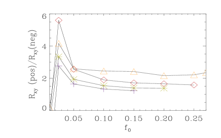
Figure 5: Ratio of the Reynolds stresses $R_{xy}$ with positive shear parameter to the ones with negative shear parameters from the hydrodynamic three-dimensional runs as function of forcing amplitude $f_{0}$. Orange color and triangles: $k_{\rm f}/k_{1}=1.5$, red color and diamonds: $k_{\rm f}/k_{1}=3$, green color and stars: $k_{\rm f}/k_{1}=5$, and violet color and crosses: $k_{\rm f}/k_{1}=10$.

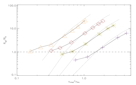
Figure 6: Reynolds stresses $R_{xy}$ generated in the MRI-unstable runs with varying forcing wavenumber and forcing amplitude, normalised to $R_{0}$, the Reynolds stress generated in the pure MRI run wihtout forcing. Orange color and triangles: $k_{\rm f}/k_{1}=1.5$, red color and diamonds: $k_{\rm f}/k_{1}=3$, green color and stars: $k_{\rm f}/k_{1}=5$, and violet color and crosses: $k_{\rm f}/k_{1}=10$. The dotted lines plotted over each curve indicate the corresponding result from purely hydrodynamic calculations with identical normalisation.

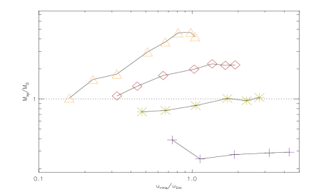
Figure 7: Maxwell stresses $M_{xy}$ generated in the MRI-unstable runs with varying forcing wavenumber and forcing amplitude, normalised to $M_{0}$, the Maxwell stress generated in the pure MRI run wihtout forcing. Colors and symbols as in Fig. 6.

Table 3: MRI-unstable runs with nonhelical forcing with resolution $64^{3}$, averages calculated over 250 rotations. The mean magnetic field $\langle B\rangle=(\langle\overline{B}_{x}^{2}\rangle^{1/2}+\langle\overline{B}_{y}^{2}\rangle)^{1/2}$, where the angular brackets denote time averages and overbar horizontal averages.

$k_{\rm f}/k_{1}$	$f_{0}$	$\langle u_{x}u_{y}\rangle$	$\mu_{0}^{-1}\langle b_{x}b_{y}\rangle$	$-M_{xy}/R_{xy}$	$u_{\rm rms}/c_{\rm s}$	$B_{\rm rms}/(\sqrt{\mu_{0}\rho_{0}}c_{\rm s})$	$\langle B\rangle/B_{\rm rms}$
Pure MRI	-	7.46 (-4)	-3.27 (-3)	4.38	0.08	0.12	0.08
1.5	0.01	8.03 (-4)	-3.33 (-3)	4.15	0.09	0.12	0.36
	0.025	1.20 (-3)	-5.13 (-3)	4.28	0.14	0.15	0.29
	0.05	1.54 (-3)	-5.81 (-3)	3.78	0.19	0.17	0.35
	0.10	3.60 (-3)	-9.68 (-3)	2.69	0.31	0.22	0.23
	0.15	6.08 (-3)	-1.21 (-2)	2.00	0.40	0.26	0.24
	0.20	9.08 (-3)	-1.51 (-2)	1.66	0.49	0.30	0.21
	0.25	1.41 (-2)	-1.52 (-2)	1.07	0.59	0.32	0.21
	0.27	1.65 (-2)	-1.37 (-2)	0.83	0.63	0.31	0.21
3	0.01	8.46 (-4)	-3.51 (-3)	4.15	0.10	0.12	0.31
	0.025	1.11 (-3)	-4.39 (-3)	3.96	0.13	0.14	0.30
	0.05	1.90 (-3)	-5.62 (-3)	2.96	0.19	0.16	0.28
	0.10	4.62 (-3)	-6.50 (-3)	1.41	0.31	0.20	0.25
	0.15	7.92 (-3)	-7.35 (-3)	0.93	0.41	0.24	0.17
	0.20	1.15 (-2)	-7.10 (-3)	0.62	0.49	0.27	0.18
	0.25	1.51 (-2)	-7.17 (-3)	0.47	0.57	0.29	0.16
5	0.01	5.99 (-4)	-2.43 (-3)	4.06	0.08	0.10	0.31
	0.025	7.82 (-4)	-2.51 (-3)	3.21	0.12	0.11	0.32
	0.05	1.63 (-3)	-2.81 (-3)	1.72	0.19	0.13	0.24
	0.10	4.23 (-3)	-3.31 (-3)	0.78	0.31	0.17	0.16
	0.15	7.34 (-3)	-3.14 (-3	0.43	0.41	0.20	0.16
	0.20	9.83 (-3)	-3.38 (-3)	0.34	0.50	0.23	0.13
10	0.01	3.40 (-4)	-1.27 (-3)	3.74	0.07	0.08	0.36
	0.025	4.60 (-4)	-8.18 (-4)	1.78	0.10	0.07	0.41
	0.05	1.15 (-3)	-9.06 (-2)	0.79	0.17	0.09	0.36
	0.10	3.03 (-3)	-9.42 (-2)	0.31	0.29	0.12	0.20
	0.15	4.66 (-3)	-9.57 (-2)	0.21	0.39	0.14	0.15

4.2.2 MRI-unstable runs

Next we turn to the magnetohydrodynamic regime and investigate a MRI-unstable setup with $k_{\rm A}/k_{1}=1$, $\Omega_{0}=0.2c_{\rm s}k_{1}$, $A_{0}=0.2\sqrt{\mu_{0}\rho_{0}}\,c_{\rm s}k_{1}^{-1}$, and $q=3/2$. For reference, we make a pure MRI-run without forcing; the results from this run are summarised in the first row of Table 3. The typical signatures of MRI (see e.g. Liljeström et al. 2009), namely a stress ratio of roughly four and magnetic energy exceeding the kinetic energy, are visible. The system does not exhibit large-scale dynamo action, so no significant mean magnetic fields are present.

As in the hydrodynamic case, we proceed by making four sets of runs with varying forcing wavenumber and amplitude; the parameters for these runs are $k_{\rm f}/k_{1}=[1.5,3,5,10]$ plotted in Figs. 6-11 with $[$violet crosses, green stars, red diamonds, orange triangles$]$, respectively. Forcing amplitudes $f_{0}$ are selected for each set separately so that turbulence levels below and above the limiting rms-velocities for MRI damping $u_{\rm lim}/c_{\rm s}=[0.6,0.3,0.18,0.09]$ are obtained at each $k_{\rm f}$; the values used and the results summarised can be found from Table 3.

In Sect. 4.2.1 it was shown that purely hydrodynamic calculations clearly produce non-zero Reynolds stresses due to shear, rotation and the adopted forcing function. Therefore, in the magnetohydrodynamic regime non-zero Maxwell stresses can also be expected to be generated by the interaction of a small-scale dynamo and shear without the MRI. Therefore, the stresses in a MRI-unstable setup can be written as

$$R_{xy} = R_{xy}^{(\rm f)}+R_{xy}^{(\rm MRI)},$$ (25)

$$M_{xy} = M_{xy}^{(\rm f)}+M_{xy}^{(\rm MRI)}.$$ (26)

Here we note that in the study of Workman & Armitage (2008) $R_{xy}^{(\rm f)}=M_{xy}^{(\rm f)}=0$ was apparently assumed in the analysis of the results. To find a definite answer to whether MRI is damped or not in the investigated setup, therefore, a techinique of separating the stresses should be developed. Before attempting that, let us first analyse the behavior of the total stresses $R_{xy}$ and $M_{xy}$ measured in our calculations.

The Reynolds stresses of the MRI-unstable calculations can well be compared to the forced hydrodynamic ones of Sect. 4.2.1; this is done in Fig. 6, where we plot both the magnetohydrodynamic stresses (solid lines with symbols) and the hydrodynamic stresses (dotted lines) normalised to the pure MRI stress. From this figure it can be seen that for the sets $k_{\rm f}/k_{1}=5$ and $10$, the weakest forcing amplitudes produce Reynolds stresses that are smaller in magnitude than the pure MRI-generated stress; this indicates that the MRI becomes reduced when external forcing is added. It is also evident that for the weakest forcings, extra stresses in addition to the hydrodynamic runs are generated by the action of MRI (the solid lines run above the dotted lines). As the strength of the turbulence grows with increasing forcing, the magnetohydrodynamic stress grows much more slowly than the hydrodynamic one, so that the two curves start approaching each other. This could be interpreted as follows: the action of the forcing on the MRI-dynamics is to decrease its contribution $R_{xy}^{(\rm MRI)}$ to the total Reynolds stress, while $R_{xy}^{(\rm f)}$ continues its growth. At the strongest forcings and the highest levels of turbulence, the hydrodynamic stress is always larger than the magnetohydrodynamic one, but the shape of the curves is almost identical; this could be interpreted as the MRI-contribution being nearly zero while $R_{xy}^{(\rm f)}$ continues its growth. These results are consistent with the scenario that the MRI becomes damped as forcing is increased, but as the curves significantly deviate from each other at high turbulence levels, this method cannot be used to definitely determine at which point the damping occurs. The stresses from hydrodynamic runs are consistently higher than those from the runs with MRI and forcing. A possible explanation is that the backreaction due to the Lorentz force quenches the Reynolds stress in the latter runs. A weak $k$-dependence can be observed: the larger the forcing wavenumber is, the smaller is the Reynolds stress which can be interpreted as an effect of the decreasing influence of shear and rotation on the system.

In contrast to the pure MRI case, in all the forced runs large-scale dynamo action develops; such a shear dynamo has been previously reported in rotating and shearing flows e.g. by Yousef et al. (2008). Due to this a mean magnetic field is generated, showing quite irregular behaviour in time disappearing and reappearing without any cyclicity. The strength of the mean magnetic field is maximally around 40 percent of the total magnetic field strength in the set $k_{\rm f}/k_{1}=10$, and minimally of the order of 10 percent with the highest forcings. Such a mean field gives a significant additional contribution to the Reynolds and Maxwell stresses. We remove this contribution using

$$\langle b_{x}b_{y}\rangle=\langle\overline{M}_{xy}^{(\rm total)}\rangle-\langle\overline{B}_{x}\rangle\langle\overline{B}_{y}\rangle,$$ (27)

where the overbars denote horizontal averaging.

For the Maxwell stress no such reference point exists as for the Reynolds stress. In Fig. 7 we simply plot the stress normalised to the pure MRI case. The behaviour of the stress is quite similar for the three smallest wavenumber sets: first the stress is growing as the forcing amplitude and turbulence level is increasing. At around $u_{\rm lim}$, the growth saturates. For the highest wavenumber set, the stress is at first strongly decreasing, but saturation is again reached around $u_{\rm lim}$. For the largest wavenumber set, the total Maxwell stress is always below the pure MRI case; also for the set $k_{\rm f}/k_{1}=5$ the stress is weaker than the pure MRI stress for the weakest forcings. This is a clear indication of the MRI-contribution to the Maxwell stress being reduced when forcing is included. If it is further assumed that the forcing-induced Maxwell stress grows monotonically as function of forcing, then the combined effect with a monotonically decreasing MRI-contribution at higher forcing amplitudes could result in the saturation of the stress; this, however, is only speculative, as no reference point is yet available. A stronger $k$-dependence compared to the Reynolds stress can be seen in the Maxwell stress: the larger the wavenumber, the smaller is the stress. There is roughly an order of magnitude difference between the Maxwell stress of $k_{\rm f}/k_{1}=1.5$ and $10$. This could be due to the decreasing value of the effective magnetic Reynolds number, ${\rm Rm}=u_{\rm rms}/(\eta k_{\rm f})$.

The energy contained in the shear flow is pumped into the magnetic energy reservoir by the Maxwell stresses; at the same time the magnetic field is being sustained by the energy from the turbulent forcing via small-scale dynamo action. As long as the MRI is capable of pumping the energy from the shear flow, the Maxwell stress normalised with the square of the rms magnetic field strength should remain more or less constant. If the MRI-activity was reduced due to the external forcing, indications of which were presented in the previous paragraph, $b_{\rm rms}$ would be expected to continue growing while the Maxwell stress gets suppressed; in Fig. 8 we plot the Maxwell stress normalised with $b^{2}_{\rm rms}$ as function of rms-velocity. For the sets $k_{\rm f}/k_{1}=[1,3,5]$ the normalised Maxwell stress is indeed constant for turbulence levels weaker than the LSA-predicted limiting value, but starts decreasing strongly for stronger turbulence. For the set $k_{\rm f}/k_{1}=10$ the Maxwell stress shows a monotonically decreasing trend, as even the weakest forcing cases are very close to $u_{\rm lim}$.

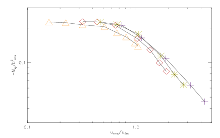
Figure 8: Maxwell stresses $-M_{xy}$ generated in the MRI-unstable runs with varying forcing wavenumber and forcing amplitude, normalised to $b^{2}_{\rm rms}$ of each run. Colors and symbols as in Fig. 6.

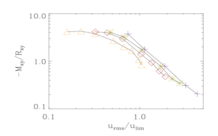
Figure 9: Maxwell to Reynolds stress ratio $-M_{xy}/R_{xy}$ as function of $u_{\rm rms}$ from MRI-unstable runs with varying forcing wavenumber and amplitude. Colors and symbols as in Fig. 6.

Keeping in mind the behavior of the individual stresses (Reynolds stress monotonically growing while Maxwell stress saturates as the forcing level is increased), one would expect the ratio of these stresses, $-M/R$, to start strongly decreasing as the level of turbulence exceeds $u_{\rm lim}$. As can be seen from Fig. 9, where we plot the stress ratio observed in each set of our calculations, the decrease of the stress ratio starts somewhat before $u_{\rm lim}$, and occurs at the same exponential rate for all the wavenumbers investigated. For the set $k_{\rm f}/k_{1}=10$, for which the widest range of $u_{\rm rms}/u_{\rm lim}$ is available, an order of magnitude decrease is observed when the weakest and strongest forcings are compared. Comparing these findings to the linear results with ordinary Ohmic diffusion $\eta$ (Sect. 4.1), indicating that the stress ratio decreases as $\eta$ increases, this behavior is indicative of MRI suppression.

To summarise, comparing the stresses developing in the forced, rotating and shearing runs to the pure MRI case does not directly give information on the suppression or enhancement of the MRI, as also the external forcing gives rise to non-zero stresses. A more appropriate way of interpreting the stresses is either to normalise them with the rms-values realised in the calculations, or to study the behavior of the stress ratio. With the help of all these diagnostics, it seems evident that the angular momentum transport due to MRI is reduced by the turbulence from external forcing, and that the functional dependence on the wavenumber seems to follow the LSA-FOSA prediction. To definitely conclude that the MRI is totally damped, a method of separating the forcng versus MRI-generated stresses should be found. This is tried in the next subsection.

Table 4: Nonhelically forced $64^{3}$ runs without MRI (shear profiles with angular velocity increasing outwards. $B_{\rm rms}$ stands for the total rms magnetic field, $\langle B\rangle$ the mean magnetic field, and $\langle b_{x}b_{y}\rangle$ are the turbulent stresses with the contribution of the mean fields removed.

$k_{\rm f}/k_{1}$	$f_{0}$	$\langle u_{x}u_{y}\rangle$	$\mu_{0}^{-1}\langle b_{x}b_{y}\rangle$	$-M_{xy}/R_{xy}$	$u_{\rm rms}/c_{\rm s}$	$B_{\rm rms}/(\sqrt{\mu_{0}\rho_{0}}c_{\rm s})$	$\langle B\rangle/B_{\rm rms}$
1.5	0.01	-2.04 (-5)	-5.49 (-5)	-2.70	0.10	0.11	0.63
	0.025	-3.77 (-5)	-3.29 (-4)	-8.72	0.14	0.07	0.34
	0.05	2.67 (-4)	-6.88 (-4)	2.58	0.20	0.08	0.20
	0.10	1.28 (-3)	-1.55 (-3)	1.20	0.32	0.13	0.18
	0.15	2.70 (-3)	-2.51 (-3)	0.93	0.42	0.17	0.16
	0.20	3.73 (-3)	-3.71 (-3)	0.99	0.50	0.21	0.16
	0.25	6.90 (-3)	-4.03 (-3)	0.58	0.61	0.23	0.17
	0.27	8.17 (-3)	-4.28 (-3)	0.52	0.64	0.25	0.17
3	0.01	-8.91 (-5)	-3.47 (-4)	-3.90	0.07	0.09	0.25
	0.025	-1.87 (-4)	-6.74 (-4)	-3.60	0.13	0.09	0.25
	0.05	1.30 (-4)	-1.49 (-3)	11.46	0.20	0.12	0.17
	0.10	2.10 (-3)	-2.11 (-3)	1.00	0.33	0.15	0.15
	0.15	4.17 (-3)	-2.98 (-3)	0.71	0.43	0.20	0.14
	0.20	6.59 (-3)	-3.61 (-3)	0.55	0.51	0.23	0.13
	0.25	1.03 (-2)	-3.62 (-3)	0.35	0.61	0.25	0.15
5	0.01	-1.13 (-4)	-3.07 (-4)	-2.71	0.08	0.11	0.41
	0.025	-1.68 (-4)	-8.46 (-4)	-5.04	0.12	0.11	0.42
	0.05	4.73 (-4)	-1.26 (-3)	2.66	0.20	0.12	0.29
	0.10	2.82 (-3)	-1.70 (-3)	0.61	0.32	0.15	0.16
	0.15	5.28 (-3)	-2.06 (-3)	0.39	0.42	0.19	0.14
	0.20	7.31 (-3)	-2.37 (-3)	0.32	0.50	0.22	0.13
10	0.01	-4.34 (-5)	-1.18 (-4)	-2.73	0.08	0.14	0.33
	0.025	-5.07 (-5)	-4.01 (-4)	-7.91	0.10	0.16	0.57
	0.05	1.56 (-4)	-7.02 (-4)	4.51	0.15	0.16	0.67
	0.10	2.02 (-3)	-8.43 (-4)	0.42	0.28	0.13	0.28
	0.15	3.82 (-3)	-8.07 (-4)	0.21	0.39	0.14	0.13

4.2.3 MRI-stable runs

We attempt to separate the stresses generated by the external forcing from the MRI-generated ones by repeating the calculations with MRI-stable shear profile for which the angular velocity is increasing outwards (the sign of the $q$-parameter is reversed, so that $q=-3/2$). All the other parameters are kept unchanged; the results from this set of calculations are summarised in Table 4.

As in the MRI-unstable calculations, the MRI-stable calculations show large-scale dynamo action due to which a mean magnetic field is generated. The negative-$q$ dynamo appears to be more efficient than the positive-$q$ one; the strength of the mean magnetic field reaches 60 percent of the total magnetic field strength in some cases. To calculate the turbulent stresses, we have removed the contribution of the mean field using Eq. (27).

For the weakest forcings, the Reynolds stress is small and negative, showing similarity to the hydrodynamic positive $q$ runs presented in Sect. 4.2.1. For stronger forcings, positive values, monotonically increasing with the forcing amplitude, are obtained. The Maxwell stress is always negative, and monotonically increasing in magnitude, but beginning to show sings of saturation for the largest forcing amplitudes. We use these stresses to normalise the ones of the MRI-unstable runs; the results are plotted in Figs. 10 and 11. The trend is quite clear for both of the stresses: for the weakest levels of turbulence, there is an excess both of Reynolds and Maxwell stresses in the MRI-unstable versus the MRI-stable case, indicative of ongoing MRI-activity. As the forcing is increased, especially the Reynolds stress quickly levels off to a roughly constant value, not showing clear correlation with the $u_{\rm lim}$. The saturation level of the Reynolds stress is close to one only in the set with the largest wavenumber $k_{\rm f}/k_{1}=10$, and increasing with decreasing $k_{\rm f}$. This can be attributed to the asymmetry $q\rightarrow-q$ observed also in the hydrodynamic calculations (Sect. 4.2.1). The Maxwell stress also shows a monotonically decreasing trend, the level-off occurring roughly at $u_{\rm lim}$. The saturation level, again, is close to unity only for the set $k_{\rm f}/k_{1}=10$, and is increasing with decreasing wavenumber. We relate this behavior to the $q\rightarrow-q$ asymmetry; due to this asymmetry, no definite conclusion about the damping limit of the MRI can be drawn even with the help of these reference calculations.

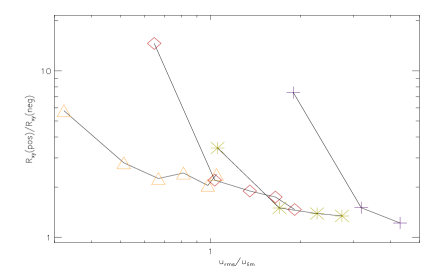
Figure 10: Reynolds stresses from the MRI-unstable runs normalised by stresses generated in the MRI-stable runs with corresponding forcing wavenumber and amplitude. Colors and symbols as in Fig. 6.

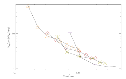
Figure 11: Maxwell stresses from the MRI-unstable runs normalised by stresses generated in the MRI-stable runs with corresponding forcing wavenumber and amplitude. Colors and symbols as in Fig. 6.

5 Application to the Milky Way

In addition to accretion disks, the disks of spiral galaxies are also subject to the MRI, as the angular velocity is decreasing outwards so that the rotational velocity is roughly constant as a function of radius outside the very centre (called as flat rotation curve, for which $q=1$). Sellwood & Balbus (1999) proposed that the MRI could be responsible of the anomalous velocity dispersions observed in the outer regions of some galaxies, and later, in a series of papers, Piontek & Ostriker showed that the MRI can really work in the cool cloudy and clumpy medium subject to thermal instability (see e.g. Piontek & Ostriker 2007). The energy balance estimates from the observations of NGC6949 (Beck 2004) indicate that magnetic energy could become dominant over the kinetic energy in the outer regions of this galaxy, so that the energy ratio $E_{\rm M}/E_{\rm K}\approx 3$–$4$. This matches well the energy ratios found from numerical simulations of MRI (e.g. Liljeström et al. 2009).

In the inner star-forming regions of spiral galaxies there is another very powerful source of turbulence in addition to the MRI, namely supernova explosions (hereafter SN). SN-forced turbulent flows have been studied numerically (e.g. Korpi et al. 1999; de Avillez & Mac Low (2002); Gressel et al. 2008), but no signs of MRI has been reported yet. Here we apply the linear analysis result together with the FOSA-prediction to obtain a preliminary estimate whether the MRI could be suppressed by SN activity.

For such an analysis, we need the rotation law for the determination of $\Omega$ and the expected growth rate of the MRI, the SN distribution as a function of radius, and the expected rms-velocity and scale of SN driven turbulence as functions of the SN forcing. For the rotation law we choose a simplified fit to the galactic rotation profile similar to the one used by Ferrière & Schmitt (2000), shown in Fig. 12. The radial distribution of SNe we obtain from the review article of Ferrière (2001), who gives

$$\sigma_{\rm I}(R) = \left(4.8\,{\rm kpc}^{-2}{\rm Myr}^{-1}\right)$$ (28)

$$\times{\rm exp}\left(-\frac{R-R_{\odot}}{4.5\,{\rm kpc}}\right)$$

$$\sigma_{\rm II}(R<3.7\,{\rm kpc}) = \left(27\,{\rm kpc}^{-2}{\rm Myr}^{-1}\right)$$ (29)

$$\times 3.55\ {\rm exp}\left(-\frac{R-3.7\,{\rm kpc}}{2.1\,{\rm kpc}}\right)^{2}$$

$$\sigma_{\rm II}(R>3.7\,{\rm kpc}) = \left(27\,{\rm kpc}^{-2}{\rm Myr}^{-1}\right)$$ (30)

$$\times{\rm exp}\left(-\frac{R^{2}-R^{2}_{\odot}}{(6.8\,{\rm kpc})^{2}}\right),$$

where $R_{\odot}=8.5$ kpc is the radius of the solar orbit.

Dib et al. (2006) investigated the velocity dispersion resulting from SNe of varying frequency in a cube of nonstratified and nonmagnetized gas. No rotation or differential rotation was included, so the system can be regarded as isotropic. SN frequencies of 0.01 to 10 times the frequency at the solar radius ($R_{\odot}=8.5$ kpc) were investigated and velocity dispersions, but no information of the scale of the turbulence, were reported. From their plots, however, it is evident that the scale is approximately 100 pc with the SN frequency at solar neighborhood. Gressel (2009) also arrives at a similar value by computing velocity structure functions from more sophisticated simulations of SN forced stratified flows. For our simple analysis, we therefore adopt the value $l_{\rm f}=100$ pc, but neglect any variation as a function of SN frequency. We then perform an approximate fit to the velocity dispersion as a function of SN frequency from the Figure 13 of Dib et al. (2006), and map the used SN frequencies over the galactic radius using the SN-distributions Eqs. (28) – (30). The resulting $\Omega_{\rm m}$ from Eq. (14) is plotted with a solid line in Fig. 12.

Finally, from the linear stability analysis, we choose $A=1.4$, corresponding to the limit where we found all the MRI-modes to be damped for $q=1$ (see Fig. 2). We show the corresponding damping curve $A\ \Gamma_{\rm max}=A/2\ \Omega(R)$ (see Eq. (15)) in Fig. 12 with a dashed line. MRI is predicted to be damped by SNe in the regions where the solid line is above the dashed line. This occurs up to the radius of roughly 13.6 kpc.

The analysis presented above can be improved by including a more realistic description of the turbulent scale and rms-velocity and their dependences, e.g.  on the interstellar magnetic field strength and surrounding density, aspects that were totally neglected here. This would require high-resolution numerical simulations of SN forced flows, involving a huge parameter space to explore. Intuitively one would expect, however, that the presence of a large-scale magnetic field and larger surrounding density would probably both result in smaller values of rms-velocities and sizes of the individual SN shells. Therefore the ratio $u_{\rm rms}/l_{\rm f}$, appearing in the Ohmic diffusion rate in the isotropic case (Eq. (14)), could remain unchanged.

Figure 12: Galactic application. An approximate fit to the galactic rotation profile (dotted line), the resulting $\Omega_{\rm m}$ from Eq. (14) (solid line), and the damping curve $A\ \Gamma_{\rm max}=A/2\ \Omega(R)$ (see Eq.15) (dashed line).

6 Conclusions

In this study we have investigated the effect of turbulent Ohmic diffusion on the excitation and dynamics of the MRI. First we presented a linear stability analysis for different types of rotation profiles of the form $\Omega\propto R^{-q}$, and proceeded by making a prediction in the isotropic homogeneous case of the level of turbulence needed to suppress MRI (Eq. (16)).

Next we made an attempt, with the help of three-dimensional numerical simulations, to investigate whether this simple criterion holds for more complex nonlinear systems. We began with purely hydrodynamic calculations with both positive (angular velocity decreasing outwards) and negative (angular velocity increasing outwards) shear parameters $q$. These calculations gave two important results: Firstly, non-zero Reynolds stresses arise solely due to the interaction of forcing, shear and rotation, in agreement with the earlier results of Snellman et al. (2009), but in apparent disagreement with the study of Workman & Armitage (2008). Secondly, there is a strongly $k_{\rm f}$-dependent asymmetry in the generated stresses in a transition $q\rightarrow-q$, so that the smaller the effective forcing wavenumber, the larger the asymmetry is in the generated Reynold stress. In the MHD regime, therefore, non-zero stresses can occur both from the forcing and the MRI, and the separation of the two contribution is very difficult, as no absolute reference point can be established due to the $q\rightarrow-q$ asymmetry.

In the magnetohydrodynamical regime sets of MRI-unstable (positive $q$) runs were made, and compared to a calculation without external forcing (exhibiting only MRI). As anticipated, the interpretation of the results without any other reference point than the pure MRI case, was difficult. Utilising the corresponding hydrodynamic calculations as reference, the MRI versus the forcing contributions to the Reynolds stress could be investigated in more reliable manner. From this analysis, indications of MRI damping were found. For the Maxwell stress, a normalisation to the rms magnetic field strength of each calculation was found to be a useful diagnostic, giving further support to the damping scenario. The Maxwell to Reynolds stress ratio was also observed to be a sensitive diagnostic of the MRI efficiency. Negative-$q$ calculations were also made in the MHD regime; due to the $q\rightarrow-q$-asymmetry of the generated stresses, these runs, however, serve as a rather poor reference point. It is possible to study this issue further with the help of nonlinear closure models, such as Ogilvie (2003) or Snellman et al. (2009). The closure model of the latter study could be used to investigate the $q\rightarrow-q$-asymmetry in more detail, whilst the former could serve as a tool to separate the two stress contributions; this, however, is out of the scope of this paper.

All in all, the effect of the external forcing on the excitation and dynamics of the MRI is to reduce its efficiency as angular momentum transport mechanism (seen both in the Reynolds and Maxwell stresses, and most clearly in their ratio), and as the turbulence level exceeds $u_{\rm lim}$, derived by linear stability analysis and the first-order smoothing approximation, to suppress the MRI-activity. To determine the exact level of turbulence at which the MRI becomes damped in the three-dimensional calculations is not possible due to the $q\rightarrow-q$-asymmetry, but according to our results, the LSA-FOSA-prediction is quite a reliable indicator.

As evident, the conclusions of our study are in complete disagreement with the very similar study of Workman & Armitage (2008). The discrepancy is mostly due to the results of the hydrodynamical calculations of both studies: our calculations clearly show non-zero $R_{xy}^{\rm f}$, whereas Workman & Armitage (2008) find very small $R_{xy}^{\rm f}$, which is interpreted to be consistent with zero. This likely to be explained by the fact that their conclusion is based on only one point although the stress varies non-monotonically as a function of $\Omega$ and $S$ (Snellman et al. 2009). Although the results of the magnetohydrodynamical calculations of both studies are in perfect agreement, the conclusions become severely altered due to the different reference points.

One particularly interesting case to apply our result is that of the star-forming inner parts of galactic disks, where the stellar turbulent energy input produces turbulence via stellar winds, radiation pressure and supernova explosions. On the other hand, the galactic disks are susceptible to the MRI with flat rotation profiles of the type $q=1$; is the stellar energy input enough to suppress the MRI, and over which range of radius does this occur? In this study we made a crude estimation utilising the LSA-FOSA-prediction together with earlier results from numerical investigations of SN forced turbulence (Korpi et al. (1999); Dib et al. (2006)) and the radial SN distribution reported in the litterature (Ferrière 2001). Our analysis gives indication that supernova activity can suppress the MRI up to the radius of roughly 14 kpc.

- [1] Ogilvie, G.I.: 2003, MNRAS 340, 969
- [2006] Pessah, M.E., Chan, C.K., Psaltis, D.: 2006, MNRAS 372, 183
- [2007] Piontek, R.A., Ostriker, E.C.: 2007, ApJ 663, 183
- [2005] Schrinner, M., Rädler, K.-H., Schmitt, D., et al.: 2005, AN 326, 245
- [2007] Schrinner, M., Rädler, K.-H., Schmitt, D., et al.: 2007, GApFD, 101, 81
- [1999] Sellwood, J.A., Balbus, S.A.: 1999, ApJ 511, 660
- [20099] Snellman, J.A., Käpylä, P.J., Korpi, M.J., Liljeström, A.J.: 2009, A&A, 505, 955
- [2008] Sur, S., Brandenburg, A., Subramanian, K.: 2008, MNRAS 385, L15
- [2008] Workman, J.C., Armitage, P.J.: 2008, ApJ 685, 406
- [1988] Wisdom, J., Tremaine, S.: 1988, AJ 95, 925
- [2008] Yousef, T.A., Heinemann, T., Rincon, F., et al.: 2008, AN 329, 737