Abstract

Two-dimensional Maxwell-Vlasov equilibria with finite electric fields, axial (“toroidal”) plasma flow and isotropic pressure are constructed in plane geometry by using the quasineutrality condition to express the electrostatic potential in terms of the vector potential. Then for Harris-type distribution functions, Ampere’s equation becomes of Liouville type and can be solved analytically. As an example, a periodic “cat-eyes” steady state consisting of a row of magnetic islands is presented. The method can be extended to (toroidal) axisymmetric equilibria.

Equilibrium is the starting point for stability and transport studies of astrophysical and laboratory plasmas. In the framework of collisionless kinetic theory, equilibrium states should be constructed as self consistent solutions of Vlasov and Maxwell equations. To this end, the knowledge of constants of motion for the particles in the continuum approximation (microfluids) is of crucial importance because then the general solution of Vlasov equation can be written as an arbitrary function of the complete set of constants of motion. This is feasible only for one-dimensional equilibria, i.e. in this case the three constants of motion are the energy ($H_{s}=(1/2)m_{s}v^{2}+q_{s}\Phi(y)$) and the two canonical momenta ($p_{xs}=m_{s}v_{x}+q_{s}A_{x}(y)$ and $p_{zs}=m_{s}v_{z}+q_{s}A_{z}(y)$); consequently, the distribution functions are of the form $f_{s}=f_{s}(H_{s},p_{xs},p_{zs})$. Here, ($x,y,z$) are Cartesian coordinates, $v^{2}=v_{x}^{2}+v_{y}^{2}+v_{z}^{2}$, $\Phi(y)$ the electrostatic potential, $A_{x}(y)$ and $A_{z}(y)$ the components of the vector potential, and the subscript $s$ denotes the particle species. Unlikely, for two-dimensional equilibria the complete set of constants of motion is missing, i.e. only the energy $H_{s}$ and the momentum $p_{zs}=m_{s}v_{z}+q_{s}A_{z}(x,y)$ conjugate to the ignorable coordinate $z$ are known out of the four constants of motion. A good number of solutions for one-dimensional [1]-[7] and two-dimensional [8]-[10] equilibria were constructed on the basis of modified Maxwellian distribution functions of the forms $f_{s}=\exp(-\beta_{s}H_{s})g_{s}(p_{xs},p_{zs})$ and $f_{s}=\exp(-\beta_{s}H_{s})g_{s}(p_{zs})$, respectively, with $g_{s}$ arbitrary functions of the conserved momenta and $\beta_{s}=1/(k_{B}T_{s})$. These equilibria concern neutral plasmas in connection with a special set of distribution functions such that it holds (for one-dimensional equilibria) $N_{i}(A_{x},A_{z})=N_{e}(A_{x},A_{z})$, where $N_{i}$ ($N_{e}$) is the ion (electron) density [1]; viz. in addition to the usual quasineutrality condition it was assumed that $N_{i}(A_{x},A_{z})$ is the same function of $A_{x}$ and $A_{z}$ as $N_{e}(A_{x},A_{z})$, thus leading to a vanishing electrostatic potential. On physical grounds this additional assumption is oversimplifying because it ignores the mass difference of ions and electrons. Also, finite electric fields associated with macroscopic plasma (ion) flows are important in laboratory fusion plasmas for the transitions from low to high confinement modes of operation.

Aim of the present study is to construct analytically a class of quasineutral, two dimensional Maxwell-Vlasov equilibria. This is accomplished by employing the quasineutrality condition (without the additional assumption of functionally identical ion and electron densities) to express $\Phi$ as a function of $A_{z}(x,y)$. A similar method was employed by Mynick and coauthors [11] to construct numerically by an iteration algorithm one-dimensional quasineutral equilibria. Also, the method was reviewed recently in Sec. II of Ref. [12].

We consider a plasma of electrons and protons at equilibrium with a current density in the axial (“toroidal”) $z$-direction. Consequently, the vector potential has a single component $A_{z}(x,y)$. In addition to the “poloidal” magnetic field with components $B_{x}(x,y)$ and $B_{y}(x,y)$ associated with $A_{z}$, we include for stabilizing reasons a constant axial magnetic field $B_{z0}$ which otherwise does not affect the equilibrium. Furthermore, we employ Harris-type distribution functions,

$$f_{s}(H_{s},p_{zs})=n_{0s}\left(\frac{m_{s}\beta_{s}}{2\pi}\right)^{3/2}\exp(-\beta_{s}H_{s})\exp(\beta_{s}V_{zs}p_{zs}),$$ (1)

where $V_{zs}$ are constant average (fluid) velocities and $n_{0s}$ reference densities corresponding to Maxwellian distribution functions ($V_{zs}=0$). Using the quasineutrality condition, $N_{i}=N_{e}$, where

$$N_{s}=n_{0s}\left(\frac{m_{s}\beta_{s}}{2\pi}\right)^{3/2}\exp(-q_{s}\beta_{s}\Phi)\int_{-\infty}^{\infty}\exp\left(-\beta_{s}m_{s}v^{2}/2\right)\exp(\beta_{s}V_{zs}p_{zs})\,d^{3}v$$

(with $q_{i}=e$ and $q_{e}=-e$), the electrostatic potential can be expressed in terms of $A_{z}(x,y)$ as

$$\Phi(A_{z})=\log\left[\frac{n_{0i}}{n_{0e}}\exp\left(A_{z}eV_{ze}\beta_{e}-\frac{1}{2}m_{e}V_{ze}^{2}\beta_{e}+A_{z}eV_{zi}\beta_{i}+\frac{1}{2}m_{i}V_{zi}^{2}\beta_{i}\right)\right]^{\frac{1}{e(\beta_{e}+\beta_{i})}}.$$ (2)

Note that for (1) all the integrations of interest in the velocity space can be performed analytically. Using (1) and (2) one finds for the current density ($j_{z}=\sum_{s}q_{s}\int_{-\infty}^{\infty}v_{z}f_{s}d^{3}v$):

$$j_{z}(A_{z})=en_{0e}^{\frac{\beta_{i}}{\beta_{e}+\beta_{i}}}n_{0i}^{1-\frac{\beta_{i}}{\beta_{e}+\beta_{i}}}\left(V_{zi}-V_{ze}\right)$$

$$\exp\left[\frac{1}{2}V_{zi}\left(2A_{z}e+m_{i}V_{zi}\right)\beta_{i}-\frac{\beta_{i}\left(A_{z}eV_{ze}\beta_{e}-\frac{1}{2}m_{e}V_{ze}^{2}\beta_{e}+A_{z}eV_{zi}\beta_{i}+\frac{1}{2}m_{i}V_{zi}^{2}\beta_{i}\right)}{\beta_{e}+\beta_{i}}\right].$$

Therefore, Ampere’s equation ($\nabla^{2}A_{z}(x,y)=-\mu_{0}j_{z}(A_{z})$) assumes a Liouville-type form

$$\nabla^{2}A_{z}=a\exp(bA_{z})$$ (4)

where

$$a = \mu_{0}\left(V_{ze}-V_{zi}\right)en_{0e}^{\frac{\beta_{i}}{\beta_{e}+\beta_{i}}}n_{0i}^{\frac{\beta_{e}}{\beta_{e}+\beta_{i}}}\exp\left[\frac{\left(m_{e}V_{ze}^{2}+m_{i}V_{zi}^{2}\right)\beta_{i}\beta_{e}}{2\left(\beta_{e}+\beta_{i}\right)}\right],$$ (5)

$$b = \frac{e\left(V_{zi}-V_{ze}\right)\beta_{e}\beta_{i}}{\beta_{e}+\beta_{i}}.$$ (6)

The equilibrium for $V_{zi}=0$ is static, viz. only the electrons are in non-thermal motion to produce the axial current. For $V_{zi}\neq 0$, however, there is a constant ion-fluid axial velocity, $\int_{-\infty}^{\infty}v_{z}f_{i}d^{3}v/N_{i}=V_{zi}$, and the ion motion contributes to $j_{z}$. It may be noted here that for distribution functions of the form $f_{s}(H_{s},p_{zs})$ it is not possible to create poloidal plasma velocities because of the two missing constants of motion. Even the third constant of motion found in Ref. [13] near the magnetic axis does not help to this end because poloidal flows vanish on axis. For the equilibrium constructed here the pressure is isotropic, i.e. the pressure tensor,

$$P_{ij}=\sum_{s}m_{z}\int_{-\infty}^{\infty}(v_{i}-\langle v_{i}\rangle_{s})(v_{j}-\langle v_{j}\rangle_{s})f_{s}d^{3}v,\ \ i,j=x,y,z,$$

is diagonal with $P_{xx}=P_{yy}=P_{zz}\equiv P$ (see also Fig. 3). For $V_{zi}=V_{ze}$ it follows that the current density vanishes ($a=b=0$) and (4) reduces to Laplace equation. Therefore, $A_{z}$ can not be constant on any closed curve in the ($x,y$) plane without being constant in the region within this curve. Consequently, the electrostatic potential $\Phi$ is constant too in this region because of (2) and the distribution functions become spatially uniform; hence, one recovers the well-known equilibrium solution of the Maxwell-Vlasov equations for which all quantities are homogeneous. No “confined solution” is possible in this case. Also, it is noted here that for $V_{zi}=V_{ze}$ solution (8) below, though pertinent to an unbounded plasma, becomes singular ($\tilde{A}_{z}\rightarrow\infty$).

Introducing dimensionless quantities ($\xi=x/L$, $\eta=y/L$, $\tilde{A}_{z}=A_{z}/(B_{z0}L)$, $\tilde{a}=aL/B_{z0}$, $\tilde{b}=bB_{z0}L$ with $L$ a length scaling parameter), the general solution of (4) is given by [14, 15]

$$\tilde{A}_{z}(x,y) = \frac{\chi\left|\tilde{a}\tilde{b}\right|-\tilde{a}\tilde{b}\log\left|\tilde{a}\tilde{b}\right|}{\tilde{a}\tilde{b}^{2}},$$

$$\chi = \log\left[\frac{\left(u^{2}+v^{2}+1\right)^{2}}{8\left(u_{\xi}^{2}+u_{\eta}^{2}\right)}\right],$$ (7)

where $u(\xi,\eta)$ and $v(\xi,\eta)$ are real conjugate functions resulting from $w(\xi+i\eta)=u+iv$, with $w$ a differentiable arbitrary generating function. As an example of complete equilibrium construction we consider here the function

$$w(\zeta)=\sqrt{\frac{1+\epsilon}{1-\epsilon}}\tan\left(\frac{\zeta}{2}\right)$$

with $\zeta=\xi+i\eta$, and $\epsilon$ a parameter such that $|\epsilon|\leq 1$. For this choice of $w$, (7) acquires the form

$$\tilde{A}_{z}(\xi,\eta)=\log\left\{\frac{2(1-\epsilon^{2})}{|\tilde{a}\tilde{b}|\left[\cosh\left(\xi\right)-\epsilon\cos\left(\eta\right)\right]^{2}}\right\}^{1/\tilde{b}}.$$ (8)

The function $\tilde{A}_{z}$ labels the magnetic surfaces. The equilibrium configuration shown in Fig. 1 consists of an infinite row of identical periodic islands known as “cat-eyes” (see for example Ref. [16]). The islands have magnetic axes at $\xi_{a}=2k\pi$, $\eta_{a}=0$ and a separatrix with $x$-points at $\xi_{x}=(2k+1)\pi$, $\eta_{x}=0$ where $k$ an integer. The ordinates of the separatrix are located at $\xi=\xi_{a}$, $\eta=\eta_{s}=\pm\ \mbox{arctanh}\left(1+2\epsilon\right)$ (see Fig. 1). The equilibrium has the following free parameters: $n_{0s}$, $\beta_{s}$, $V_{zs}$ ($s=e,i$), $B_{z0}$, $\epsilon$, and $L$. The dependent parameters $a$ and $b$ (Eqs. (5 and (6)) relate features of the distribution function to macroscopic equilibrium characteristics (Eq. (8)). For $V_{zi}\neq V_{ze}$ the physical quantities (${\mathbf{B}}$, ${\mathbf{E}}=-(d\Phi/dA_{z})\nabla A_{z}$, $j_{z}$ and $P$) are everywhere regular and vanish as $y$ tends to infinity except for $E_{y}$ which in this limit approaches a finite value. Profiles of $E_{x}$ and $E_{y}$ are shown in Fig. 2 for the following fusion relevant values of the free parameters: $n_{0i}=n_{0e}=10^{19}m^{-3}$, $k_{B}T_{i}=k_{B}T_{e}=1keV$, $V_{zi}=10^{4}m/sec$, $V_{ze}=10V_{zi}$, $B_{z0}=1T$, $L=1m$, and $\epsilon=0.6$. Also, the $y$-profiles of $j_{z}$ and $P$ have an extremum on the magnetic axis (Fig. 3). For $\epsilon=0$ the configuration becomes one-dimensional; this is as an extension of the Harris sheet equilibrium [17] (usually employed as initial state in reconnection studies) with finite $\bf E$ and constant axial velocity.

Quasineutral equilibria with sheared axial flow which may be more pertinent to the improved confinement modes can be constructed by the alternative distribution functions

$$f_{s}(H_{s},p_{zs})=n_{0s}\left(\frac{m_{s}\beta_{s}}{2\pi}\right)^{3/2}\exp(-\beta_{z}H_{s})\exp\left(\frac{\beta_{zs}p_{zs}^{2}}{2m_{s}}\right),$$ (9)

with $\beta_{s}$ and $\beta_{zs}$ constants. A similar procedure then leads to $A_{z}$-dependent average axial velocities:

$$\frac{\int_{-\infty}^{\infty}v_{z}f_{s}d^{3}v}{N_{s}}=\frac{q_{s}\beta_{zs}}{m_{s}(\beta_{s}-\beta_{zs})}A_{z}(x,y),$$

and Ampere’s equation assumes the form

$$\nabla^{2}A_{z}=a_{1}A_{z}\exp\left(b_{1}A_{z}^{2}\right),$$ (10)

where the parameters $a_{1}$ and $b_{1}$ are known functions of $n_{0s}$, $\beta_{s}$ and $\beta_{zs}$. Eq. (10), higher nonlinear than (4), should be solved numerically.

In summary, using the quasineutrality condition to express the electrostatic potential in terms of the vector potential and Harris-type distribution functions (Eq. (1)) we have constructed a class of plane, two-dimensional Maxwell-Vlasov equilibria with finite electric fields, constant axial plasma velocity and isotropic pressure. The equilibrium was exemplified by the cat-eyes solution. Equilibria with sheared axial flow can be derived by alternative distribution functions, e.g. (9). The method can also be applied in (toroidal) axisymmetric and helically symmetric geometries.

One of the authors (GNT) would like to thank Prof. H. Weitzner for useful discussions. Part of this work was conducted during a visit of GNT to the Max-Planck-Institut für Plasmaphysik, Garching. The hospitality of that Institute is greatly appreciated. This work was performed within the participation of the University of Ioannina in the Association Euratom-Hellenic Republic, which is supported in part by the European Union and by the General Secretariat of Research and Technology of Greece. The views and opinions expressed herein do not necessarily reflect those of the European Commission.

Fig. 1:  $\tilde{A}_{z}$-lines of the cat-eyes solution (7) as intersections of the magnetic surfaces with the poloidal plane.

Fig. 2:  Profiles of the electric field components $E_{x}$ and $E_{y}$ associated with the cat-eyes solution (7). The profiles $E_{x}(y)$ and $E_{y}(x)$ have chosen at $x/L=\pi/2$ and $y/L=0.5$, respectively, because $E_{x}(x=0,y)=E_{y}(x,y=0)\equiv 0$.

Fig. 3:   $y$-profiles at $x=0$ of the current density, $j_{z}$, and the pressure, $P$, associated with the cat-eyes solution (7).

List of Figures

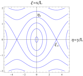
Figure 1: $\tilde{A}_{z}$-lines of the cat-eyes solution (7) as intersections of the magnetic surfaces with the poloidal plane.

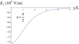
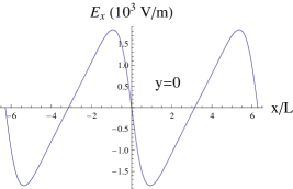
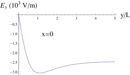
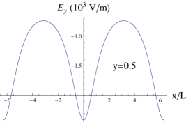
Figure 2: Profiles of the electric field components $E_{x}$ and $E_{y}$ associated with the cat-eyes solution (7). The profiles $E_{x}(y)$ and $E_{y}(x)$ have chosen at $x/L=\pi/2$ and $y/L=0.5$, respectively, because $E_{x}(x=0,y)=E_{y}(x,y=0)\equiv 0$.

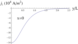
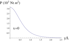
Figure 3: $y$-profiles at $x=0$ of the current density, $j_{z}$, and the pressure, $P$, associated with the cat-eyes solution (7).

References

- [1] Paul J. Channell, Phys. Fluids 19, 1541 (1976).
- [2] Swadesh M. Mahajan, Phys. Fluids B 1, 43 (1989).
- [3] N. Attico, F. Pegoraro, Phys. Plasmas 6, 767 (1999).
- [4] F. Mottez, Phys. Plasmas 10, 2501 (2003).
- [5] F. Mottez, Ann. Geophys. 22, 3033 (2004).
- [6] C. Montagna and F. Pegoraro, Phys. Plasmas 14, 042103 (2007).
- [7] Michael G. Harrison and Thomas Neukirch PRL 102, 135003 (2009).
- [8] F. Ceccherini, C. Montagna, F. Pegoraro, G. Cicogna, Phys. Plasmas 12, 052506 (2005).
- [9] Akihiro Suzuki and Toshikazu Shigeyama, Phys. Plasmas 15, 042107 (2008).
- [10] Akihiro Suzuki Phys. Plasmas 15, 072107 (2008).
- [11] Harry E. Mynick, William M. Sharp, and A. N. Kaufman, Phys. Fluids. 22, 1478 (1979).
- [12] Michael G. Harrison and Thomas Neukirch Phys. Plasmas 16, 022106 (2009).
- [13] H. Tasso and G. N. Throumoulopoulos, J. Phys. A: Math. Theor. 40, F631 (2007).
- [14] J. Liouville, J. Math. 18 (1), 71 (1853).
- [15] Roberto A. Clemente, Int. J. Math. Educ. Sci. Technol. 23, 620 (1992).
- [16] G. N. Throumoulopoulos, H. Tasso, G. Poulipoulis, J. Phys. A: Math. Theor. 42, 335501 (2009).
- [17] E. G. Harris, Nuovo Cimento 23, 115 (1962).
Figure captions