Resonant and Kondo tunneling through molecular magnets

Abstract

Transport through molecular magnets is studied in the regime of strong coupling to the leads. We consider a resonant-tunneling model where the electron spin in a quantum dot or molecule is coupled to an additional local, anisotropic spin via exchange interaction. The two opposite regimes dominated by resonant tunneling and by Kondo transport, respectively, are considered. In the resonant-tunneling regime, the stationary state of the impurity spin is calculated for arbitrarily strong molecule-lead coupling using a master-equation approach, which treats the exchange interaction perturbatively. We find that the characteristic fine structure in the differential conductance persists even if the hybridization energy exceeds thermal energies. Transport in the Kondo regime is studied within a diagrammatic approach. We show that magnetic anisotropy gives rise to the appearance of two Kondo peaks at nonzero bias voltages.

I Introduction

Over the past few years the idea of integrating the concepts of spintronics and molecular electronics has developed into a new research field dubbed molecular spintronics.Sanvito ; Bogani Progress has not only been stimulated by technological interests but has also been accompanied by the realization that magnetic single-molecule transistors exhibit various fundamental quantum phenomena.Park ; Jo ; Heersche ; Grose ; Tejada ; Durkan ; Rugar Among many promising ideas discussed in the literature, particular attention has been paid to current-induced spin reading and writing, spin relaxation, entanglement, quantum computation, and Kondo correlations.Romeike ; Elste ; Misiorny1 ; Misiorny2 ; Braun ; Barraza-Lopez ; Souza ; Jonckheere ; Lu ; Lindebaum

An experimental realization of spintronics devices may be achieved by using single-molecule magnets in combination with metallic (nonmagnetic or ferromagnetic) leads. For molecular-memory applications, long spin-relaxation times are advantageous, which may be realized in molecules with large magnetic anisotropy, such as molecules based on $\mathrm{Mn}_{12}$, $\mathrm{Fe}_{4}$, and $\mathrm{Ni}_{4}$.Blundell ; Sangregorio ; Mannini

Controlling and detecting the molecular spin by means of electronic tunneling into source and drain electrodes poses a major challenge. While some approaches rely on break junctions, others are based on a scanning tunneling microscope. In both cases, the coupling between the molecule and the leads can vary by several orders of magnitude, thus giving rise to strikingly different transport regimes.Park ; Jo ; Heersche ; Grose ; Nitzan ; Xue ; Joachim ; Donarini ; Zhou ; Yu ; Emberly2 ; Koch ; Fang ; Koerting

In the regime of weak molecule-lead coupling, many experimental features such as Coulomb blockade, spin blockade, sequential tunneling, and cotunneling can be described within a master-equation or rate-equation approach treating the electronic tunneling perturbatively.Timm However, for strong coupling, low-order perturbation theory breaks down. It is then advantageous to treat the electronic tunneling exactly, at the price of introducing approximations elsewhere.

Recently, the Kondo effect in single-molecule magnets with easy-axis anisotropy has been studied by Romeike et al.Romeike Their model describes an anisotropic spin coupled to metallic electrodes by an exchange interaction, in the absence of a bias voltage. This differs from the model studied here, in which the electronic spin in the relevant molecular orbital is coupled to an additional local, anisotropic spin via an exchange interaction $J$, i.e., charge fluctuations are explicitly taken into account. In addition, we include a nonzero bias voltage. The presence of a Kondo effect for an anisotropic spin is at first glance surprising since it requires two approximately degenerate low-energy spin states connected by a term in the Hamiltonian. The simplest Hamiltonian for an anisotropic spin $\mathbf{S}$ with $S\geq 1$ exchange-coupled to an electronic spin $\mathbf{s}$

$$H=-K_{2}(S^{z})^{2}+J\,\mathbf{s}\cdot\mathbf{S}$$ (1)

does not provide such a term. Using a renormalization-group approach, Romeike et al.Romeike could show that quantum tunneling of the magnetic moment, which is described by higher-order anisotropy terms not included in Eq. (1), may give rise to a Kondo peak in the linear conductance, centered at zero bias voltage. The Kondo temperature is found to depend strongly on the ratio of the applied magnetic field and the anisotropy barrier. Further, González et al.Gonzalez have derived a Kondo Hamiltonian of the type studied in Ref. Romeike, from an electronic model. They have shown that a transverse magnetic field can induce or quench the Kondo effect. This is due to Berry-phase interference between different quantum tunneling paths of the spin.

Koerting et al.Koerting consider the nonequilibrium Kondo effect for a double quantum dot with four leads. By removing the leads coupled to one of the dots one would obtain a model similar to ours. The main difference is that we include charge fluctuations on the dot which is coupled to the leads, whereas Koerting et al.Koerting work in the regime of weak tunneling and Coulomb blockade, where both quantum dots act as local spins.

In the present paper, we address the question of spin-dependent resonant tunneling and Kondo tunneling through molecular magnets. As noted above, we consider a resonant-tunneling model where the electron spin on the quantum dot or molecule is coupled to an additional local, anisotropic spin via an exchange interaction $J$. We assume this interaction to be weak, which allows us to employ perturbation theory for small $J$. The stationary current through the left and right leads is identical and is related to the local electronic spectral function $A_{\sigma}(\omega)$ on the molecule by the Meir-Wingreen formulaMeir

$$\langle I_{L}\rangle=\frac{e}{2\pi\hbar}\sum_{\sigma}\int d\omega\,\frac{\Gamma_{L}\Gamma_{R}}{\Gamma_{L}+\Gamma_{R}}\left[f_{L}(\omega)-f_{R}(\omega)\right]\,A_{\sigma}(\omega),$$ (2)

where $\sigma$ is the spin, $\Gamma_{\alpha}$ is the broadening of the molecular level due to the hybridization with lead $\alpha=L,R$, to be defined below, and $f_{\alpha}$ denotes the Fermi distribution function of lead $\alpha$. The spectral function is determined by the imaginary part of the retarded Green’s function, $A_{\sigma}(\omega)=-2\,\text{Im}G^{\text{ret}}_{\sigma\sigma}(\omega)$. If transport is dominated by a single molecular level of energy $\varepsilon_{d}$, the coupling to the leads gives rise to a Lorentzian form of the spectral function, $A^{0}_{\sigma}(\omega)=\Gamma/[(\omega-\varepsilon_{d})^{2}+\Gamma^{2}/4]$ with $\Gamma=\Gamma_{L}+\Gamma_{R}$, which manifests itself as a peak in the differential conductance. For single-molecule devices, the excitation of additional degrees of freedom due to the electronic tunneling is expected to translate into additional characteristic features in the current.

We consider two complementary situations. The first is the case of arbitrary gate and bias voltages but excluding the region where the Kondo contribution to the current is large. Within a master-equation approach treating the local exchange interaction perturbatively to second order, we calculate the transition rates between local-spin states, showing that the spin can be driven out of equilibrium even for strong molecule-lead hybridization. Signatures of inelastic tunneling such as the fine-structure splitting of the differential-conductance peaks persist in the regime where the hybridization energy exceeds the thermal energy.

The second case concerns the regime of a large Kondo contribution to the differential conductance, which only occurs for small bias voltages on the order of $|eV|\sim K_{2}(2S-1)$, as we shall see. Here, transport is studied using a diagrammatic approach. We consider the case that the molecular orbital is far from resonance so that the resonant-tunneling contributions are negligible. In addition, this allows us to obtain analytical expressions. We find that the magnetic anisotropy gives rise to the appearance of two Kondo peaks in the differential conductance at finite bias voltages $\pm V_{c}$. This intrinsically nonequilibrium Kondo effect is quite different from the zero-bias peak studied by Romeike et al.,Romeike which relies on higher-order anisotropies absent from our model. In our case, the magnetic anisotropy acts like a magnetic field in that it gives rise to a splitting of the Kondo peak. Furthermore, we find a suppression of the differential conductance with $1/\varepsilon_{d}^{6}$.

The paper is organized as follows. In Sec. II, we introduce our model. Section III considers transport within a master-equation approach, which allows us to study magnetic nonequilibrium phenomena, whereas Sec. IV considers a diagrammatic approach, which applies to the Kondo regime. In Sec. V we summarize and discuss our results further. Some detailed calculations are relegated to Appendices.

II Model

We consider a magnetic molecule coupled to two metallic leads. Electronic tunneling through the junction is assumed to involve a single orbital with energy $\varepsilon_{d}$ and spin $\mathbf{s}$ that is coupled to a local spin S via exchange interaction. The model is described by the Hamiltonian

$$H=H_{0}+H_{J}+H_{\text{mag}},$$ (3)

where

$$H_{0}~{}=~{} \varepsilon_{d}\sum_{\sigma}d^{\dagger}_{\sigma}d_{\sigma}+\sum_{\alpha\mathbf{k}\sigma}\epsilon_{\alpha\mathbf{k}}\,a^{\dagger}_{\alpha\mathbf{k}\sigma}a_{\alpha\mathbf{k}\sigma}$$

$$+\sum_{\alpha\mathbf{k}\sigma}\left(t_{\alpha}\,a^{\dagger}_{\alpha\mathbf{k}\sigma}d_{\sigma}+t^{*}_{\alpha}\,d^{\dagger}_{\sigma}a_{\alpha\mathbf{k}\sigma}\right)$$ (4)

is the resonant-tunneling Hamiltonian,

$$H_{J}=J\,\mathbf{s}\cdot\mathbf{S}$$ (5)

with $\mathbf{s}\equiv\sum_{\sigma\sigma^{\prime}}d^{\dagger}_{\sigma}({\mbox{\boldmath$\sigma$}_{\sigma\sigma^{\prime}}}/{2})d_{\sigma^{\prime}}$ is the exchange interaction between the electrons in the molecular orbital and the local spin $\mathbf{S}$, and

$$H_{\text{mag}}=-K_{2}(S^{z})^{2}$$ (6)

describes the easy-axis magnetic anisotropy of the local spin. We choose the z axis as the easy axis. Here, $d^{\dagger}_{\sigma}$ creates an electron with spin $\sigma$ and energy $\varepsilon_{d}$ on the molecule, while $a^{\dagger}_{\alpha\mathbf{k}\sigma}$ creates an electron with energy $\epsilon_{\alpha\mathbf{k}}$, wave vector $\mathbf{k}$, and spin $\sigma$ in lead $\alpha$, which is considered a noninteracting electron gas. The vector $\mbox{\boldmath$\sigma$}\equiv(\sigma_{x},\sigma_{y},\sigma_{z})$ denotes the Pauli matrices. In break junctions produced by electromigration, the onsite energy $\varepsilon_{d}$ can be tuned by applying a gate voltage.Park ; Jo ; Heersche ; Grose

III Master equation for the spin

The presence of strong coupling between the molecule and the leads prevents us from treating the hybridization term in Eq. (II) perturbatively. However, since the Hamiltonian becomes bilinear in the limit of vanishing exchange coupling, $J=0$, our strategy is to diagonalize $H_{0}+H_{\text{mag}}$ exactly while treating $H_{J}$ as a perturbation up to second order. This approach allows us to study the nonequilibrium dynamics of the molecular spin at finite bias voltages for arbitrary molecule-lead coupling strengths, provided that Kondo correlations do not lead to a diverging contribution from higher-order terms in the expansion.

We start by rewriting $H_{0}$ in terms of new operators,Mahan ; Mitra

$$H_{0}=\sum_{\alpha\mathbf{k}\sigma}\epsilon_{\alpha\mathbf{k}}\,c^{\dagger}_{\alpha\mathbf{k}\sigma}c_{\alpha\mathbf{k}\sigma},$$ (7)

where

$$a_{\alpha\mathbf{k}\sigma} = \sum_{\alpha^{\prime}\mathbf{k}^{\prime}}\eta^{\alpha\mathbf{k}}_{\alpha^{\prime}\mathbf{k}^{\prime}}c_{\alpha^{\prime}\mathbf{k}^{\prime}\sigma},$$ (8)

$$d_{\sigma} = \sum_{\alpha\mathbf{k}}\nu_{\alpha\mathbf{k}}c_{\alpha\mathbf{k}\sigma},$$ (9)

and

$$\eta^{\alpha\mathbf{k}}_{\alpha^{\prime}\mathbf{k}^{\prime}} = \delta_{\alpha\alpha^{\prime}}\delta_{\mathbf{k}\mathbf{k}^{\prime}}-\frac{t_{\alpha}\nu_{\alpha^{\prime}\mathbf{k}^{\prime}}}{\epsilon_{\alpha\mathbf{k}}-\epsilon_{\alpha^{\prime}\mathbf{k}^{\prime}}+i\,\delta},$$ (10)

$$\nu_{\alpha\mathbf{k}} = \frac{t_{\alpha}}{\epsilon_{\alpha\mathbf{k}}-\varepsilon_{d}-\sum_{\alpha^{\prime}\mathbf{k}^{\prime}}\frac{t_{\alpha^{\prime}}^{2}}{\epsilon_{\alpha\mathbf{k}}-\epsilon_{\alpha^{\prime}\mathbf{k}^{\prime}}-i\,\delta}}.$$ (11)

For simplicity we assume real tunneling amplitudes $t_{\alpha}$. In terms of the new operators, the exchange interaction assumes the form

$$H_{J}=J\sum_{\alpha\alpha^{\prime}\mathbf{k}\mathbf{k}^{\prime}\sigma\sigma^{\prime}}\nu_{\alpha\mathbf{k}}^{*}\nu_{\alpha^{\prime}\mathbf{k}^{\prime}}\,c^{\dagger}_{\alpha\mathbf{k}\sigma}\frac{\mbox{\boldmath$\sigma$}_{\sigma\sigma^{\prime}}}{2}c_{\alpha^{\prime}\mathbf{k}^{\prime}\sigma^{\prime}}\cdot\mathbf{S}.$$ (12)

The time evolution of the density matrix $\rho$ of the full system is described by the von Neumann equation, $\dot{\rho}=-(i/\hbar)[H,\rho]$. The degrees of freedom of the local spin are described by the reduced density matrix

$$\rho_{J}=\text{Tr}_{\text{el}}\,\rho,$$ (13)

which is obtained by tracing out all electronic degrees of freedom. Assuming that the large electronic subsystem, which acts as a spin reservoir, is weakly perturbed by the exchange coupling, we replace the full density matrix by the direct product $\rho\simeq\rho_{J}\otimes\rho_{\text{el}}$. We need a further approximation for the electronic density matrix $\rho_{\text{el}}$. We assume that different chemical potentials $\mu_{L}$ ($\mu_{R}$) are imposed for the left (right) lead far from the junction. It would thus be natural to assume Fermi distributions $f_{\alpha}(\omega)=f(\omega-\mu_{\alpha})$ for the physical electrons created by $a_{\alpha\mathbf{k}\sigma}^{\dagger}$. However, we need to make a reasonable assumption on the transformed c fermions appearing in Eqs. (7) and (12). Since $c^{\dagger}_{L\mathbf{k}\sigma}$ ($c^{\dagger}_{R\mathbf{k}\sigma}$) creates an electron in a state with vanishing probability density far from the junction in the right (left) lead, we assume the occupation numbers of these states to be described by $f_{\alpha}(\omega)$.

Making use of the Markov approximation that $\rho_{J}$ changes slowly on the time scale of electronic relaxation, we obtain

$$\dot{\rho}_{J}(t)=-\frac{1}{\hbar^{2}}\int_{-\infty}^{t}dt^{\prime}\,\text{Tr}_{\text{el}}\,\left[H_{J}(t),\left[H_{J}(t^{\prime}),\rho_{J}(t)\otimes\rho_{\text{el}}\right]\right].$$ (14)

Here, operators $O(t)$ with an explicit time argument, including $\rho_{J}(t)$, are in the interaction picture, $O(t)=e^{i(H_{0}+H_{\text{mag}})t/\hbar}\,O\,e^{-i(H_{0}+H_{\text{mag}})t/\hbar}$. Note that second-order perturbation theory in the exchange coupling gives the first non-vanishing correction to the conductance, since the expectation value $\langle\textbf{S}\rangle$ and thus all first-order terms vanish exactly due to symmetry.

We are interested in the stationary state. The stationary density matrix $\rho_{J}$ has to be diagonal in the basis of eigenstates $|m\rangle$ of $S^{z}$, since the full Hamiltonian $H$ is invariant under rotation about the z-axis in spin space. Inserting Eq. (12) into Eq. (14) we thus obtain a Pauli master equation, also called rate equations, of the form

$$\dot{P}_{m}~{}=~{} P_{m+1}R_{m+1\rightarrow m}+P_{m-1}R_{m-1\rightarrow m}$$

$$~{}-P_{m}\left(R_{m\rightarrow m+1}+R_{m\rightarrow m-1}\right)~{}=~{}0$$ (15)

for the occupation probabilities $P_{m}$ of spin states $|m\rangle$ in the stationary state. The transition rates read

$$R_{m\to m\pm 1}=|\langle m\pm 1|S^{\pm}|m\rangle|^{2}\,\frac{J^{2}/4}{2\pi\hbar}$$ (16)

$${}\times\sum_{\alpha\alpha^{\prime}}\int d\omega\,|\tilde{\nu}_{\alpha}(\omega)|^{2}\,|\tilde{\nu}_{\alpha^{\prime}}(\omega-[\pm 2m+1]K_{2})|^{2}$$

$${}\times\left[1-f_{\alpha}(\omega)\right]f_{\alpha^{\prime}}(\omega-[\pm 2m+1]K_{2}).$$

The spectral functions are given by

$$|\tilde{\nu}_{\alpha}(\omega)|^{2}=\frac{\Gamma_{\alpha}}{(\omega-\varepsilon_{d})^{2}+\Gamma^{2}/4}$$ (17)

with $\Gamma\equiv\Gamma_{L}+\Gamma_{R}$ and $\Gamma_{\alpha}\equiv 2\pi t_{\alpha}^{2}D_{\alpha}$. The densities of states for the leads, $D_{\alpha}$, are taken as constants. Compared to Eq. (11) we have approximated the self-energy part of $\nu_{\alpha\mathbf{k}}$ by a constant and absorbed a factor $2\pi D_{\alpha}$.

At zero temperature, the integrals can be evaluated analytically. In the limit of large bias voltages, the rates approach the constant value

$$R_{m\rightarrow m\pm 1} = \frac{\pi J^{2}\,\Gamma_{L}\Gamma_{R}}{2\pi\hbar\,\Gamma\left[\Gamma^{2}+(\pm 2m+1)^{2}K_{2}^{2}\right]}$$ (18)

$${}\times|\langle m\pm 1|S^{\pm}|m\rangle|^{2}.$$

On the other hand, at zero bias only the rates involving the absorption of energy are finite, whereas the emission rates vanish.

Solving Eq. (III) allows us to compute the differential conductance of the molecular junction. The current operator of lead $\alpha$ reads

$$I_{\alpha}=-i\frac{e}{\hbar}\sum_{\mathbf{k}\sigma}t_{\alpha}\left(a^{\dagger}_{\alpha\mathbf{k}\sigma}d_{\sigma}-d^{\dagger}_{\sigma}a_{\alpha\mathbf{k}\sigma}\right)$$

$$=i\frac{e}{\hbar}\sum_{\mathbf{k}\sigma}\!\sum_{\alpha^{\prime}\mathbf{k}^{\prime}\alpha^{\prime\prime}\mathbf{k}^{\prime\prime}}\!\!\Big{(}t_{\alpha}\nu_{\alpha^{\prime}\mathbf{k}^{\prime}}^{*}\eta^{\alpha\mathbf{k}}_{\alpha^{\prime\prime}\mathbf{k}^{\prime\prime}}c^{\dagger}_{\alpha^{\prime}\mathbf{k}^{\prime}\sigma}c_{\alpha^{\prime\prime}\mathbf{k}^{\prime\prime}\sigma}-\text{h.c.}\Big{)}.$$

In order to compute the spin-dependent contribution to the expectation value $\langle I_{\alpha}\rangle\equiv\text{Tr}\,I_{\alpha}\rho=\text{Tr}\,I_{\alpha}(t)\rho(t)$ of the total current, we use the iterative solution of the von Neumann equation,

$$\rho(t)=-\frac{1}{\hbar^{2}}\int_{-\infty}^{t}dt^{\prime}\int_{-\infty}^{t^{\prime}}dt^{\prime\prime}\left[H_{J}(t^{\prime}),\left[H_{J}(t^{\prime\prime}),\rho(t^{\prime\prime})\right]\right].$$ (20)

A term containing $\rho(-\infty)$ has dropped out here since it is linear in $H_{J}$ and thus vanishes upon taking the trace. Making use of the Markov approximation we find

$$\langle I_{\alpha}\rangle^{(2)}~{}=~{} -\frac{1}{\hbar^{2}}\int_{-\infty}^{t}dt^{\prime}\int_{-\infty}^{t^{\prime}}dt^{\prime\prime}$$

$$\times\text{Tr}\,\left[\left[I_{\alpha}(t),H_{J}(t^{\prime})\right],H_{J}(t^{\prime\prime})\right]\rho(t)$$ (21)

for the second-order term. Carrying out the time integrals and evaluating the spin sums as explained in Appendix A, we obtain

$$\langle I_{L}\rangle^{(2)}=\frac{e}{2\pi\hbar}\,\frac{J^{2}}{4}\sum_{\alpha\alpha^{\prime}\alpha^{\prime\prime}}\Big{(}\Gamma_{L}-\delta_{L\alpha}\left[\Gamma_{L}+\Gamma_{R}\right]\Big{)}$$ (22)

$${}\times\sum_{m}P_{m}\,\bigg{\{}\frac{1}{2}\,|\langle m-1|S^{-}|m\rangle|^{2}I_{\alpha\alpha^{\prime}\alpha^{\prime\prime}}([-2m+1]K_{2})$$

$$\quad{}+\frac{1}{2}\,|\langle m+1|S^{+}|m\rangle|^{2}I_{\alpha\alpha^{\prime}\alpha^{\prime\prime}}([2m+1]K_{2})$$

$$\quad{}+|\langle m|S^{z}|m\rangle|^{2}I_{\alpha\alpha^{\prime}\alpha^{\prime\prime}}(0)\bigg{\}}$$

with

$$I_{\alpha\alpha^{\prime}\alpha^{\prime\prime}}(E)\equiv\int d\omega\,|\tilde{\nu}_{\alpha^{\prime\prime}}(\omega)|^{2}$$

$${}\times\Big{\{}|\tilde{\nu}_{\alpha}(\omega)|^{2}\,|\tilde{\nu}_{\alpha^{\prime}}(\omega-E)|^{2}\,\left[1-f_{\alpha}(\omega)\right]f_{\alpha^{\prime}}(\omega-E)$$

$$\quad{}-|\tilde{\nu}_{\alpha}(\omega)|^{2}\,|\tilde{\nu}_{\alpha^{\prime}}(\omega+E)|^{2}\,f_{\alpha}(\omega)\left[1-f_{\alpha^{\prime}}(\omega+E)\right]\Big{\}}.$$

Equations (22) and (III) give the first non-vanishing correction to the zero-order current $\langle I_{L}\rangle^{(0)}$, which is obtained from the Meir-Wingreen formula [Eq. (2)] by inserting the spectral function of the unperturbed system, $A^{0}_{\sigma}(\omega)=\Gamma/[(\varepsilon_{d}-\omega)^{2}+\Gamma^{2}/4]$. Note that Eq. (2) with $A_{\sigma}=A^{0}_{\sigma}$ is recovered by inserting the equilibrium density matrix $\rho^{0}$ and the current operator from Eq. (III) into $\langle I_{L}\rangle^{0}=\text{Tr}\,I_{L}\,\rho^{0}$.

A simple interpretation of Eq. (22) is possible for the special case of a local spin of length $S=1/2$, for which the magnetic anisotropy $K_{2}$ is irrelevant and can be set to zero. For this case we obtain

$$\langle I_{L}\rangle^{(2)} ~{}=~{}\frac{e}{2\pi\hbar}\,\frac{J^{2}S(S+1)}{4}\,\frac{\Gamma_{L}\Gamma_{R}}{\Gamma}$$

$$\times\int d\omega\left[\frac{\Gamma}{(\omega-\varepsilon_{d})^{2}+\Gamma^{2}/4}\right]^{3}\,\left[f_{L}(\omega)-f_{R}(\omega)\right].$$ (24)

Here, the third power of the spectral function appears, since the current operator and the two exchange-interaction operators in Eq. (III) are each bilinear in fermionic operators.

$\begin{array}[]{cc}\textbf{(a)}\\ \includegraphics[height=156.49014pt,angle={0}]{figa_symmetric.eps}\\ \textbf{(b)}\\ \includegraphics[height=156.49014pt,angle={0}]{figb_symmetric.eps}\end{array}$

Figure 1: (Color online) (a) Current-voltage characteristics for different hybridization energies, $\Gamma=K_{2}/20$, $\Gamma=K_{2}/10$, and $\Gamma=K_{2}$. The inset shows a closeup of the fine structure at positive bias. (b) Magnetic transition rates $R_{2\rightarrow 1}$, $R_{1\rightarrow 0}$ and occupation probabilities $P_{m}$ as functions of bias $V$ for $\Gamma=K_{2}/20$. We assume symmetric couplings to the leads, $\Gamma_{L}=\Gamma_{R}$, and symmetric capacitances, $\mu_{L}=eV/2$, $\mu_{R}=-eV/2$, a local molecular spin of length $S=2$, $\varepsilon_{d}=4K_{2}$, and zero temperature. Further, we set $J=\Gamma/5$. Currents are given in units of $(2e/\hbar)\Gamma_{L}\Gamma_{R}/\Gamma$. Rates are given in units of their maximum values, cf. Eq. (18).

$\begin{array}[]{cc}\textbf{(a)}\\ \includegraphics[height=156.49014pt,angle={0}]{figa_asymmetric.eps}\\ \textbf{(b)}\\ \includegraphics[height=156.49014pt,angle={0}]{figb_asymmetric.eps}\end{array}$

Figure 2: (Color online) (a) Current-voltage characteristics for different hybridization energies, $\Gamma=K_{2}/20$, $\Gamma=K_{2}/10$, and $\Gamma=K_{2}$. The inset shows a closeup of the fine structure at positive bias. (b) Magnetic transition rates $R_{2\rightarrow 1}$, $R_{1\rightarrow 0}$ and occupation probabilities $P_{m}$ as functions of bias $V$ for $\Gamma=K_{2}/20$. We assume strongly asymmetric couplings to the leads, $\Gamma_{L}\ll\Gamma_{R}$, and strongly asymmetric capacitances, $\mu_{L}=eV$, $\mu_{R}=0$, a local molecular spin of length $S=2$, $\varepsilon_{d}=4K_{2}$, and zero temperature. Further, we set $J=\Gamma/5$. Currents are given in units of $(2e/\hbar)\Gamma_{L}\Gamma_{R}/\Gamma$. Rates are given in units of their maximum values, cf. Eq. (18).

If the magnetic anisotropy is large compared to the hybridization energy, $K_{2}\gg\Gamma$, the general expression for the current in Eq. (22) simplifies to

$$\langle I_{L}\rangle^{(2)}=~{} \frac{e}{2\pi\hbar}\,\frac{J^{2}}{4}\sum_{\alpha\alpha^{\prime}\alpha^{\prime\prime}}\!\!\Big{(}\Gamma_{L}-\delta_{L\alpha}\left[\Gamma_{L}+\Gamma_{R}\right]\Big{)}I_{\alpha\alpha^{\prime}\alpha^{\prime\prime}}(0)$$

$$~{}\times\sum_{m}P_{m}|\langle m|S^{z}|m\rangle|^{2},$$ (25)

since the integrals $I_{\alpha\alpha^{\prime}\alpha^{\prime\prime}}([\pm 2m+1]K_{2})$ are negligible compared to $I_{\alpha\alpha^{\prime}\alpha^{\prime\prime}}(0)$. Assuming symmetric capacitances, one finds, in the limit of large bias voltages,

$$\langle I_{L}\rangle^{(0)} \to \frac{2e}{\hbar}\,\frac{\Gamma_{L}\Gamma_{R}}{\Gamma},$$ (26)

$$\langle I_{L}\rangle^{(2)} \to \frac{2e}{\hbar}\,\frac{\Gamma_{L}\Gamma_{R}}{\Gamma}\,\frac{3S(S+1)}{4}\,\frac{J^{2}}{\Gamma^{2}},$$ (27)

for the zero-order and second-order contribution, respectively. Note that the ferromagnetic or antiferromagnetic sign of $J$ does not affect the results in the present approximation.

We first consider the situation of symmetric molecule-lead couplings and capacitances, i.e., $|t_{L}|=|t_{R}|$, $\Gamma_{L}=\Gamma_{R}$, and $\mu_{L}=eV/2$, $\mu_{R}=-eV/2$. Figure 1(a) shows the current-voltage characteristics up to second order in $J$ for the case of a local spin of length $S=2$. The characteristic fine structure of the current step at the Coulomb-blockade threshold is due to the second-order contribution, $\langle I_{L}\rangle^{(2)}$, whereas the main step is mostly coming from $\langle I_{L}\rangle^{(0)}$. The fine structure persists as long as the hybridization energy $\Gamma$ remains small compared to the magnetic anisotropy $K_{2}$. Note that the broadening of the steps is due to $\Gamma>0$, and not to the temperature, for which we assume $T\ll\Gamma$. For bias voltages below $|eV|=2\varepsilon_{d}$, the current and all magnetic excitations are thermally suppressed. However, as soon as the chemical potential of one lead aligns with the resonance of the molecule, the current increases to its maximum value. The current-induced magnetic transitions become energetically accessible at the same time, as shown in Fig. 1(b), resulting in nonequilibrium probabilities $P_{m}$ of the different spin states. In the limit of large bias voltages all spin states are equally occupied, $P_{m}=1/(2S+1)$.

Interestingly, the presence of magnetic anisotropy leads to negative differential conductance in the vicinity of $|eV|=2\varepsilon_{d}$. The underlying mechanism shall be explained briefly. According to Eq. (III), the magnetic states with maximum quantum numbers $m=\pm S$ dominate the current since the current is proportional to the average $\sum_{m}P_{m}|\langle m|S^{z}|m\rangle|^{2}$. Each decrease in $P_{\pm S}$ thus causes a decrease in the current. Therefore, the spin-dependent contribution to the current is large at low bias voltages, where $P_{\pm 2}=1/2$ and $\sum_{m}P_{m}m^{2}=4$, and small at high bias voltages, where $P_{\pm 2}=1/5$ and $\sum_{m}P_{m}m^{2}=2$.

$\begin{array}[]{c}\textbf{(a)}\\ \includegraphics[height=119.50148pt,angle={0}]{levelscheme.eps}\\ \begin{array}[]{cc}\textbf{(b)}&\hskip 5.69046pt\textbf{(c)}\\ \includegraphics[height=119.50148pt,angle={0}]{current2D_symmetric.eps}&\includegraphics[height=119.50148pt,angle={0}]{current2D_asymmetric.eps}\end{array}\end{array}$

Figure 3: (Color online) (a) Level scheme showing all spin transitions to order $J^{2}$. (b),(c) Two-dimensional density plots of the absolute value of the second-order current contribution $\langle I_{L}\rangle^{(2)}$ as a function of bias voltage $V$ and gate potential $\varepsilon_{d}$ for $\Gamma=K_{2}/20$. $\varepsilon_{d}$ is controlled by the gate voltage. We choose the same parameters as in Fig. 1. Bright (dark) colors correspond to high (low) currents. In (b) we assume symmetric couplings, $\mu_{L}=eV/2$, $\mu_{R}=-eV/2$, $\Gamma_{L}=\Gamma_{R}$, while in (c) we assume asymmetric couplings, $\mu_{L}=eV$, $\mu_{R}=0$, $\Gamma_{R}\gg\Gamma_{L}$.

We next consider the situation of strongly asymmetric molecule-lead couplings and capacitances, i.e., $|t_{L}|\ll|t_{R}|$, $\Gamma_{L}\ll\Gamma_{R}$, and $\mu_{L}\simeq eV$, $\mu_{R}\simeq 0$. Note that this regime is naturally realized in many experimental setups, whereas perfectly symmetric couplings are in general more difficult to achieve. The current-voltage curves and the bias dependence of the magnetic excitation rates are shown in Fig. 2. Due to the asymmetric coupling and $\varepsilon_{d}>0$, the current is suppressed for negative bias voltages. However, the characteristic steps corresponding to excitations of the molecular spin reappear at positive bias. Only their abscissas are reduced by a factor of 2, since the chemical potential of the left lead is now $\mu_{L}=eV$ instead of $\mu_{L}=eV/2$. The device thus acts as a rectifier. Note the small ohmic contribution with constant slope for large coupling $\Gamma$ in Fig. 2(a). We return to this point below.

We finally turn to the full bias and gate-voltage dependence of the current. In both the symmetric and the asymmetric case, selection rules for the spin require changes in the magnetic quantum number by $\Delta m=0$ or $\Delta m=\pm 1$, where $\Delta m=0$ corresponds to elastic and $\Delta m=\pm 1$ to inelastic scattering events, cf. Fig. 3(a). Inelastic scattering processes appear as additional steps in the current and give rise to the magnetic fine structure in the two dimensional density plots of the second-order contribution to the current as a function of bias and gate voltages shown in Figs. 3(b), (c). We can now understand the origin of the weak ohmic conduction seen in Fig. 2(a) for $\Gamma=K_{2}$. What we are seeing is the tail of the current step at $\epsilon_{d}=0$ in Fig. 3(c), which is considerably broadened for $\Gamma=K_{2}$. Note that we here have $\epsilon_{d}=4K_{2}=4\Gamma$, i.e., we are only $4\Gamma$ away from the step. Since this distance does not depend on the bias voltage, the conductivity is essentially constant, leading to ohmic behavior.

IV Kondo transport

Second-order perturbation theory in the exchange interaction $J$ fails, even for small $J$, if the prefactors of higher-order terms diverge. This is the case in the Kondo regime. Logarithmic divergences of the conductance first appear in terms of third order in $J$.Ng ; Glazman ; Goldhaber-Gordon ; Cronenwett ; Wiel (In this section, we assume antiferromagnetic exchange, $J>0$.) Studying the emergence of Kondo correlations thus requires to go beyond the second-order master-equation approach discussed in Sec. III. For sufficiently small $J$ and sufficiently large thermal energies, the conductance is dominated by the third-order contribution, which we calculate in this section. At lower temperatures, it would become necessary to resum the divergences to all orders in $J$.Ng ; Glazman ; Goldhaber-Gordon ; Cronenwett ; Wiel

The total current through the molecule is related to the local electronic spectral function $A_{\sigma}(\omega)=-2\text{Im}G^{\textit{ret}}_{\sigma\sigma}(\omega)$ by the Meir-Wingreen formula, Eq. (2), where $G_{\sigma\sigma^{\prime}}^{\text{ret}}(\omega)=\int d(t-t^{\prime})\,e^{i\omega(t-t^{\prime})}G_{\sigma\sigma^{\prime}}^{\text{ret}}(t-t^{\prime})$ denotes the Fourier transform of the retarded single-particle Green’s function

$$G^{\text{ret}}_{\sigma\sigma^{\prime}}(t,t^{\prime})\equiv-i\theta(t-t^{\prime})\big{\langle}\big{\{}d_{\sigma}(t),d^{\dagger}_{\sigma^{\prime}}(t^{\prime})\big{\}}\big{\rangle}.$$ (28)

Making use of the transformation defined in Eqs. (8)–(11) requires to compute the finite-temperature time-ordered Green’s function

$$\mathcal{G}_{\alpha\alpha^{\prime}\textbf{k}\textbf{k}^{\prime}\sigma\sigma^{\prime}}(\tau,\tau^{\prime})\equiv-\big{\langle}T_{\tau}\,c_{\alpha\textbf{k}\sigma}(\tau)c^{\dagger}_{\alpha^{\prime}\textbf{k}^{\prime}\sigma^{\prime}}(\tau^{\prime})\big{\rangle}.$$ (29)

Our strategy is to expand $\mathcal{G}_{\alpha\alpha^{\prime}\textbf{k}\textbf{k}^{\prime}\sigma\sigma^{\prime}}$ in powers of $J$.

In order to obtain the current from the Meir-Wingreen formula, we need the imaginary part of the electronic Green’s function,

$$\text{Im}\sum_{\sigma}G^{\text{ret}}_{\sigma\sigma}(\omega)=\text{Im}\sum_{\alpha\alpha^{\prime}\textbf{k}\textbf{k}^{\prime}\sigma}\nu_{\alpha\mathbf{k}}\nu_{\alpha^{\prime}\mathbf{k}^{\prime}}^{*}\mathcal{G}^{\text{ret}}_{\alpha\alpha^{\prime}\textbf{k}\textbf{k}^{\prime}\sigma\sigma}(\omega),$$ (30)

where $\mathcal{G}^{\text{ret}}_{\alpha\alpha^{\prime}\textbf{k}\textbf{k}^{\prime}\sigma\sigma}(\omega)$ denotes the retarded Green’s function. All non-vanishing diagrams of the local Green’s function up to third order in $J$ are shown in Fig. 4, following the notation of Ref. Bruus, . We again consider the case of strongly asymmetric couplings, i.e., $|t_{L}|\ll|t_{R}|$, $\Gamma_{L}\ll\Gamma_{R}$, and $\mu_{L}\simeq eV$, $\mu_{R}\simeq 0$. As we shall see, Eq. (30) is then dominated by the contribution from the right electrode, $\alpha=\alpha^{\prime}=R$. This allows us to describe the molecular degrees of freedom by a thermal equilibrium distribution function that is independent of the applied bias voltage and to obtain an analytical expression.

Figure 4: Non-vanishing diagrams of the impurity Green’s function up to third order in $J$, following Ref. Bruus, . Diagrams including fermion loops vanish exactly and are not shown. Spin averages are denoted by dotted lines.

The evaluation of Eq. (30) is shown in Appendix B. We obtain

$$\text{Im}\sum_{\sigma}G^{\text{ret}}_{\sigma\sigma}(\omega)\simeq-\frac{\Gamma/2}{\varepsilon_{d}^{2}+\Gamma^{2}/4}+\left(\frac{\varepsilon_{d}}{\varepsilon_{d}^{2}+\Gamma^{2}/4}\right)^{\!2}\text{Im}\Sigma^{\text{ret}}(\omega)$$ (31)

with

Im $$\Sigma^{\text{ret}}(\omega)~{}=~{}-\frac{\pi}{2}J^{2}\nu_{0}(\varepsilon_{d})\sum_{mnl}P_{m}\,\frac{1-f(\omega+E_{m}-E_{l})}{1-f(\omega)}\,\Bigg{\{}\delta_{nl}\sum_{i}|\langle m|S^{i}|n\rangle|^{2}$$

$$-iJ\nu_{0}(\varepsilon_{d})\sum_{ijk}\epsilon_{ijk}\langle m|S^{i}|n\rangle\langle n|S^{j}|l\rangle\langle l|S^{k}|m\rangle\bigg{[}\ln\bigg{|}\frac{x}{\sqrt{(\omega+E_{m}-E_{n})^{2}+T^{2}}}\bigg{|}+\ln\bigg{|}\frac{x}{\sqrt{(\omega+E_{n}-E_{l})^{2}+T^{2}}}\bigg{|}\bigg{]}\Bigg{\}},$$ (32)

where

$$\nu_{0}(\varepsilon_{d})=\frac{\Gamma/2\pi}{\varepsilon_{d}^{2}+\Gamma^{2}/4}.$$ (33)

In the derivation we have assumed the molecular level to be far from resonance, i.e., $|\varepsilon_{d}|$ to be large compared to $K_{2}S$, $T$, and $\Gamma$, but still small compared to the band width $x$ of the leads. Details are discussed in Appendix B. We have also assumed $|\omega|\ll|\varepsilon_{d}|$, the significance of which will become clear in the following step. Under these conditions, the resonant-tunneling contribution to the differential conductance, which we have studied in Sec. III, is negligible compared to the Kondo contribution.

In the low-temperature limit $T\ll\Gamma$, derivatives of the Fermi functions with respect to the bias voltage become delta functions and the differential conductance simplifies to

$$G\simeq\frac{e^{2}}{2\pi\hbar} \,\frac{\Gamma_{L}\Gamma_{R}}{\Gamma}\,\Bigg{\{}\frac{\Gamma}{\varepsilon_{d}^{2}+\Gamma^{2}/4}$$

$$-2\left(\frac{\varepsilon_{d}}{\varepsilon_{d}^{2}+\Gamma^{2}/4}\right)^{2}\,\text{Im}\,\Sigma^{\text{ret}}(eV)\Bigg{\}}.$$ (34)

Note that the argument $\omega$ of $\Sigma^{\text{ret}}(\omega)$ is $eV$. The assumption $|\omega|\ll|\varepsilon_{d}|$ made above thus corresponds to $|\varepsilon_{d}|$ also being large compared to the bias, $|eV|$. The spectral function has logarithmic divergences for $T\to 0$ at the transition energies of the molecule, $E_{m}-E_{n}$, corresponding to virtual transitions between two magnetic states $|m\rangle$ and $|n\rangle$. One recovers the prefactor $3\pi J^{2}D_{0}/8$, see Ref. Bruus, , for the case of spin $S=1/2$ and the (then irrelevant) anisotropy set to $K_{2}=0$.

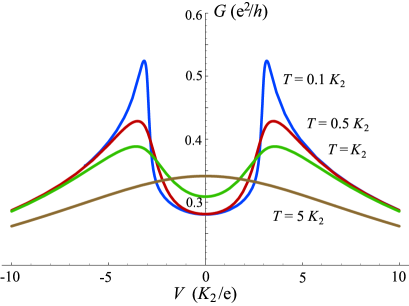
Figure 5: (Color online) Differential conductance $G$ in units of $e^{2}/h$ for different thermal energies $T$ (in units of $K_{2}$) obtained from Eq. (IV) as a function of bias voltage $V$ in units of $K_{2}/e$. Here we assume a local molecular spin of length $S=2$ and choose $J\nu_{0}(\varepsilon_{d})=1$, $x=100\,K_{2}$, and $\Gamma_{R}=100\,\Gamma_{L}$. Note that the parameters $\Gamma$, $\varepsilon_{d}$, and $J$ leave the curves for $G$ (in arbitrary units) invariant except for changing the constant offset.

Numerical results for nonzero temperatures are shown in Fig. 5. The differential conductance $G$ diverges logarithmically for $T\to 0$ at critical bias voltages $V=\pm V_{c}$ with $eV_{c}=E_{S-1}-E_{S}=K_{2}(2S-1)$ since the emergence of Kondo correlations requires the bias voltage to exceed the energy of the transition from the ground states, $m=\pm S$, to the first excited states, $m=\pm(S-1)$. Note that $G(V)$ is symmetric for positive and negative bias, in spite of the highly asymmetric coupling since it is probing the electronic spectral function. The situation is quite different from the case considered by Romeike et al.,Romeike which concerns a zero-bias peak resulting from quantum tunneling between the two states $|S\rangle$ and $|{-S}\rangle$. In our case, the splitting of the Kondo peak as a consequence of magnetic anisotropy is more similar to the situation of a quantum dot in an external magnetic field with Zeeman energy $B$, where a Zeeman splitting of the energy levels leads to the occurrence of two conductance peaks at $eV\simeq\pm B$ in the Kondo regime.Paaske3 At higher temperatures, $T\gg K_{2}$, the two Kondo peaks merge into a single peak centered at zero bias due to the thermal excitation of spin states with higher energy.

We now turn to the Kondo temperature $T_{K}$. Poor man’s scaling for the equilibrium case results in $T_{K}=0$ because the matrix elements of $S^{\pm}$ between the two degenerate ground states of the local spin vanish for our model if $S>1/2$.Romeike Since a Kondo effect evidently does occur at nonzero bias, this result is clearly not sufficient. A rough estimate of the Kondo temperature $T_{K}$ can be obtained as the temperature for which the second-order and third-order terms become equal in Eq. (IV). We find $T_{K}\sim\exp[-1/\alpha\nu_{0}(\varepsilon_{d})J]$, where $\alpha$ is a number of the order of unity. In the limit $K_{2}\to 0$, where the two peaks in Fig. 5 would merge, we recover the result $\alpha=2$ for an isotropic spin.

Since we focus on the case of strongly asymmetric couplings, where the molecular degrees of freedom are in equilibrium with one of the two leads, the logarithmic divergences are cut off by temperature or the applied bias voltage, respectively, in our perturbative approach, see Eq. (IV). The divergence for $T\to 0$ is unphysical and would likely be removed by a resummation of higher-order terms. By analogy to Ref. Paaske3, , we conjecture that the divergence is ultimately cut off by a voltage-dependent spin-relaxation rate.

While we have so far discussed the dependence on the bias voltage, see Fig. 5, we now turn to the gate voltage. The gate voltage shifts the on-site energy $\varepsilon_{d}$ and thus enters the expression for the current through the square of the spectral function $\Gamma/[\varepsilon_{d}^{2}+\Gamma^{2}/4]$ and the square of the factor $\varepsilon_{d}/[\varepsilon_{d}^{2}+\Gamma^{2}/4]$. In particular, we obtain a suppression of $G\propto 1/\varepsilon_{d}^{6}$ in the limit of strong detuning, $\varepsilon_{d}\gg\Gamma$.

V Conclusions

We have studied the spin-dependent electronic transport through magnetic molecules for strong coupling to the leads. Our discussion has focused on two complementary regimes.

For the first regime, we have presented a description of transport in terms of a master equation that keeps the electronic tunneling exactly, holds for arbitrary bias and gate voltages, and treats the local exchange interaction $J$ perturbatively at second order. This approach is thus applicable for small $J$. We have derived the bias-dependent magnetic transition rates showing that the tunneling current can be used to drive the molecular spin out of equilibrium. Further, we have shown that the characteristic fine structure of the differential-conductance peaks persists for strong molecule-lead coupling, where the broadening of the peaks is determined by the hybridization energies.

The perturbative expansion in $J$ fails if Kondo correlations contribute significantly to the transport. In this case, prefactors of the third- and higher-order terms in $J$ diverge for $T\to 0$. The Kondo correlations can become important for small bias voltages on the order of $|eV|\sim K_{2}(2S-1)$. Here, transport is described by the Meir-Wingreen formula in combination with a diagrammatic calculation of the local electronic spectral function of the molecule. We have assumed the molecular level to be far from resonance, which on the one hand makes sure that the resonant-tunneling contributions to the conductance are small and which on the other allows us to obtain analytical results. We have shown that Kondo peaks appear at finite bias voltages proportional to the anisotropy energy of the molecular spin.

Our results leave several avenues for future research. First, it would be interesting to include a local Coulomb interaction $U$ between the electrons on the molecule. However, due to the large hybridization there are no states with large probability on the dot and the effect of $U$ is expected to be relatively weak. We expect that for very large $U$ an equilibrium Kondo resonance could occur as a zero-bias peak in the differential conductance in addition to the nonequilibrium Kondo effect described in this paper. Second, the presence of an external magnetic field might lead to an interesting interplay with the splitting of the Kondo peaks due to the magnetic anisotropy. Finally, it would be desirable to combine the two cases studied here and to analyze the Kondo effect in magnetic molecules in the resonant-tunneling regime, where resonant-tunneling contributions to the conductance are not negligible and the spin is driven out of equilibrium by the current.

Appendix A Calculation of the current

In this appendix we give details on the derivation of Eqs. (22) and (III). We start from Eq. (III),

$$\langle I_{\alpha}\rangle^{(2)}~{}=~{} -\frac{1}{\hbar^{2}}\int_{-\infty}^{t}dt^{\prime}\int_{-\infty}^{t^{\prime}}dt^{\prime\prime}$$

$$\times\text{Tr}\,\left[\left[I_{\alpha}(t),H_{J}(t^{\prime})\right],H_{J}(t^{\prime\prime})\right]\rho(t).$$ (35)

Inserting the expressions for the current operator $I_{\alpha}$, Eq. (LABEL:currentI), and for the exchange interaction $H_{J}$, Eq. (12), we find

$$\langle I_{L}\rangle^{(2)}=i\frac{e}{\hbar}\frac{t_{L}J^{2}}{4\hbar^{2}}\int_{-\infty}^{t}\!\!\!dt^{\prime}\int_{-\infty}^{t^{\prime}}\!\!\!dt^{\prime\prime}\,\text{Tr}\,\sum_{\textbf{k}\sigma}\sum_{123456}\delta_{\sigma\sigma_{1}}\delta_{\sigma_{1}\sigma_{2}}$$ (36)

$${}\times\bigg{(}\eta^{L\textbf{k}*}_{1}\nu_{2}\nu_{3}^{*}\nu_{4}\nu_{5}^{*}\nu_{6}-\nu_{1}^{*}\eta^{L\textbf{k}}_{2}\nu_{3}^{*}\nu_{4}\nu_{5}^{*}\nu_{6}\bigg{)}$$

$${}\times\bigg{[}\left[c^{\dagger}_{1}(t)c_{2}(t),c^{\dagger}_{3}(t^{\prime})c_{4}(t^{\prime})\,\mbox{\boldmath$\sigma$}_{\sigma_{3}\sigma_{4}}\cdot\mathbf{S}(t^{\prime})\right],$$

$$\quad c^{\dagger}_{5}(t^{\prime\prime})c_{6}(t^{\prime\prime})\mbox{\boldmath$\sigma$}_{\sigma_{5}\sigma_{6}}\cdot\mathbf{S}(t^{\prime\prime})\bigg{]}\rho(t),\hskip 80.00012pt$$

where we have assumed $t_{L}$ to be real. Here, the shorthand notation $j=1,2,3,4,5,6$ stands for $(\alpha_{j},\mathbf{k}_{j},\sigma_{j})$.

Introducing $\tau=t-t^{\prime}$ and $\tau^{\prime}=t^{\prime}-t^{\prime\prime}$ and assuming a product state gives

$$\langle I_{L}\rangle^{(2)}=i\frac{e}{\hbar}\frac{t_{L}J^{2}}{4\hbar^{2}}\int_{0}^{\infty}d\tau\int_{0}^{\infty}d\tau^{\prime}\,\sum_{\textbf{k}}\sum_{123456}\big{(}\eta^{L\textbf{k}*}_{1}\nu_{2}\nu_{3}^{*}\nu_{4}\nu_{5}^{*}\nu_{6}-\nu_{1}^{*}\eta^{L\textbf{k}}_{2}\nu_{3}^{*}\nu_{4}\nu_{5}^{*}\nu_{6}\big{)}$$ (37)

$${}\times\Big{\{}\big{[}\delta_{23}\delta_{45}\delta_{16}f_{2}f_{4}\left(1-f_{6}\right)e^{i(\epsilon_{6}-\epsilon_{2})\tau/\hbar}e^{i(\epsilon_{6}-\epsilon_{4})\tau^{\prime}/\hbar}-\delta_{14}\delta_{25}\delta_{36}f_{2}\left(1-f_{4}\right)\left(1-f_{6}\right)e^{i(\epsilon_{4}-\epsilon_{2})\tau/\hbar}e^{i(\epsilon_{6}-\epsilon_{2})\tau^{\prime}/\hbar}$$

$$\qquad{}-\delta_{14}\delta_{25}\delta_{36}f_{2}f_{4}\left(1-f_{6}\right)e^{i(\epsilon_{4}-\epsilon_{2})\tau/\hbar}e^{i(\epsilon_{6}-\epsilon_{2})\tau^{\prime}/\hbar}+\delta_{23}\delta_{45}\delta_{16}\left(1-f_{2}\right)f_{4}\left(1-f_{6}\right)e^{i(\epsilon_{6}-\epsilon_{2})\tau/\hbar}e^{i(\epsilon_{6}-\epsilon_{4})\tau^{\prime}/\hbar}\big{]}$$

$$\qquad{}\times\text{Tr}_{J}\,2\,\mathbf{S}(0)\cdot\mathbf{S}(-\tau^{\prime})\,\rho_{J}$$

$$\quad{}-\big{[}\delta_{23}\delta_{45}\delta_{16}f_{2}\left(1-f_{4}\right)f_{6}e^{i(\epsilon_{6}-\epsilon_{2})\tau/\hbar}e^{i(\epsilon_{6}-\epsilon_{4})\tau^{\prime}/\hbar}-\delta_{14}\delta_{25}\delta_{36}\left(1-f_{2}\right)\left(1-f_{4}\right)f_{6}e^{i(\epsilon_{4}-\epsilon_{2})\tau/\hbar}e^{i(\epsilon_{6}-\epsilon_{2})\tau^{\prime}/\hbar}$$

$$\qquad{}-\delta_{14}\delta_{25}\delta_{36}\left(1-f_{2}\right)f_{4}f_{6}e^{i(\epsilon_{4}-\epsilon_{2})\tau/\hbar}e^{i(\epsilon_{6}-\epsilon_{2})\tau^{\prime}/\hbar}+\delta_{23}\delta_{45}\delta_{16}\left(1-f_{2}\right)\left(1-f_{4}\right)f_{6}e^{i(\epsilon_{6}-\epsilon_{2})\tau/\hbar}e^{i(\epsilon_{6}-\epsilon_{4})\tau^{\prime}/\hbar}\big{]}$$

$$\qquad{}\times\text{Tr}_{J}\,2\,\mathbf{S}(0)\cdot\mathbf{S}(\tau^{\prime})\,\rho_{J}\Big{\}}.$$

This result can be rewritten as

$$\langle I_{L}\rangle^{(2)}=i\frac{e}{\hbar}\frac{t_{L}J^{2}}{4\hbar^{2}}\int_{0}^{\infty}\!\!d\tau\int_{0}^{\infty}\!\!d\tau^{\prime}\,\sum_{\textbf{k}}\sum_{123456}\big{(}\eta^{L\textbf{k}*}_{1}\nu_{2}\nu_{3}^{*}\nu_{4}\nu_{5}^{*}\nu_{6}-\nu_{1}^{*}\eta^{L\textbf{k}}_{2}\nu_{3}^{*}\nu_{4}\nu_{5}^{*}\nu_{6}\big{)}$$

$$\!\!{}\times\Big{\{}\big{[}\delta_{23}\delta_{45}\delta_{16}f_{4}\left(1-f_{6}\right)e^{i(\epsilon_{6}-\epsilon_{2})\tau/\hbar}e^{i(\epsilon_{6}-\epsilon_{4})\tau^{\prime}/\hbar}-\delta_{14}\delta_{25}\delta_{36}f_{2}\left(1-f_{6}\right)e^{i(\epsilon_{4}-\epsilon_{2})\tau/\hbar}e^{i(\epsilon_{6}-\epsilon_{2})\tau^{\prime}/\hbar}\big{]}\text{Tr}_{J}\,2\,\mathbf{S}(0)\cdot\mathbf{S}(-\tau^{\prime})\,\rho_{J}$$

$$\!\!{}-\big{[}\delta_{23}\delta_{45}\delta_{16}\left(1-f_{4}\right)f_{6}e^{i(\epsilon_{6}-\epsilon_{2})\tau/\hbar}e^{i(\epsilon_{6}-\epsilon_{4})\tau^{\prime}/\hbar}-\delta_{14}\delta_{25}\delta_{36}\left(1-f_{2}\right)f_{6}e^{i(\epsilon_{4}-\epsilon_{2})\tau/\hbar}e^{i(\epsilon_{6}-\epsilon_{2})\tau^{\prime}/\hbar}\big{]}\text{Tr}_{J}\,2\,\mathbf{S}(0)\cdot\mathbf{S}(\tau^{\prime})\,\rho_{J}\Big{\}}.$$

The sums over spin indices are simplified by making use of the identities

$$\sum_{\sigma\sigma^{\prime}}\mbox{\boldmath$\sigma$}_{\sigma\sigma^{\prime}}\cdot\mathbf{S}_{1}\,\mbox{ \boldmath$\sigma$}_{\sigma^{\prime}\sigma}\cdot\mathbf{S}_{2} = 2\,\mathbf{S}_{1}\cdot\mathbf{S}_{2},$$

$$\sum_{\sigma\sigma^{\prime}}\mbox{\boldmath$\sigma$}_{\sigma\sigma^{\prime}}\cdot\mathbf{S}_{1}\,\mbox{ \boldmath$\sigma$}_{\sigma^{\prime},-\sigma}\cdot\mathbf{S}_{2} = 0.$$ (39)

In the coefficients $\nu_{\alpha\mathbf{k}}$ in Eq. (11), we approximate the self-energy part by a constant, as we did in Sec. III,

$$\nu_{\alpha\mathbf{k}}=\nu_{\alpha}(\epsilon_{\alpha\mathbf{k}})\simeq\frac{t_{\alpha}}{\epsilon_{\alpha\mathbf{k}}-\varepsilon_{d}-i\Gamma/2}.$$ (40)

Noting that Eqs. (10) and (11) imply

$$\sum_{\textbf{k}}\,\eta^{L\textbf{k}}_{1}=\delta_{L\alpha_{1}}+i\pi D_{L}t_{L}\nu_{\alpha_{1}}(\epsilon_{1})$$ (41)

and

$$\nu_{\alpha}(\epsilon)-\nu_{\alpha}(\epsilon)^{*}=i\frac{\Gamma}{t_{\alpha}}\,|\nu_{\alpha}(\epsilon)|^{2},$$ (42)

we arrive at the following expression for the tunneling current:

$$\langle I_{L}\rangle^{(2)}=i\frac{e}{\hbar}\frac{t_{L}J^{2}}{4\hbar^{2}}\int_{0}^{\infty}\!d\tau\int_{0}^{\infty}\!d\tau^{\prime}\sum_{123456}\big{[}\left(\delta_{L\alpha_{1}}-i\pi D_{L}t_{L}\nu_{1}^{*}\right)\nu_{2}\nu_{3}^{*}\nu_{4}\nu_{5}^{*}\nu_{6}-\nu_{1}^{*}\left(\delta_{L\alpha_{2}}+i\pi D_{L}t_{L}\nu_{2}\right)\nu_{3}^{*}\nu_{4}\nu_{5}^{*}\nu_{6}\big{]}$$

$$\!\!{}\times\Big{\{}\big{[}\delta_{23}\delta_{45}\delta_{16}f_{4}\left(1-f_{6}\right)e^{i(\epsilon_{6}-\epsilon_{2})\tau/\hbar}e^{i(\epsilon_{6}-\epsilon_{4})\tau^{\prime}/\hbar}-\delta_{14}\delta_{25}\delta_{36}f_{2}\left(1-f_{6}\right)e^{i(\epsilon_{4}-\epsilon_{2})\tau/\hbar}e^{i(\epsilon_{6}-\epsilon_{2})\tau^{\prime}/\hbar}\big{]}\text{Tr}_{J}\,2\,\mathbf{S}(0)\cdot\mathbf{S}(-\tau^{\prime})\,\rho_{J}$$

$$\!\!{}-\big{[}\delta_{23}\delta_{45}\delta_{16}\left(1-f_{4}\right)f_{6}e^{i(\epsilon_{6}-\epsilon_{2})\tau/\hbar}e^{i(\epsilon_{6}-\epsilon_{4})\tau^{\prime}/\hbar}-\delta_{14}\delta_{25}\delta_{36}\left(1-f_{2}\right)f_{6}e^{i(\epsilon_{4}-\epsilon_{2})\tau/\hbar}e^{i(\epsilon_{6}-\epsilon_{2})\tau^{\prime}/\hbar}\big{]}\text{Tr}_{J}\,2\,\mathbf{S}(0)\cdot\mathbf{S}(\tau^{\prime})\,\rho_{J}\Big{\}}.$$

Since we have assumed $\rho_{J}$ to be diagonal in the stationary state, we finally obtain Eqs. (22) and (III).

Appendix B Calculation of the impurity Green’s function

In order to use the Meir-Wingreen formula for the conductance, we have to compute the imaginary part of the Green’s function in Eq. (30). We consider the situation of strongly asymmetric molecule-lead couplings and capacitances, i.e., $|t_{L}|\ll|t_{R}|$, $\Gamma_{L}\ll\Gamma_{R}$, and $\mu_{L}\simeq eV$, $\mu_{R}\simeq 0$.

Since Wick’s theorem does not apply to spin operators, averages of products of spin operators do not factorize into averages of pairs. We follow Ref. Bruus, in evaluating the spin averages. Expanding the electronic Matsubara-Green’s function in powers of $J$ and organizing the expansion in terms of topologically distinct diagrams, one obtainsBruus

$$\mathcal{G}_{\alpha\alpha^{\prime}\textbf{k}\textbf{k}^{\prime}\sigma\sigma^{\prime}}(\tau,\tau^{\prime}) =\sum_{n=0}^{\infty}\left(-\frac{J}{\hbar}\right)^{n}\int_{0}^{\beta}d\tau_{1}\cdots\int_{0}^{\beta}d\tau_{n}\sum_{i_{1}\cdots i_{n}}\sum_{\sigma_{1}\cdots\sigma_{n},\sigma^{\prime}_{1}\cdots\sigma^{\prime}_{n}}\Big{\langle}T_{\tau}\left[S^{i_{1}}(\tau_{1})\cdots S^{i_{n}}(\tau_{n})\right]\Big{\rangle}_{0}$$

$$~{}~{}\times\bigg{\langle}T_{\tau}\left[B^{\dagger}_{\sigma_{1}}(\tau_{1})\frac{\mbox{\boldmath$\sigma$}_{\sigma_{1}\sigma^{\prime}_{1}}}{2}B_{\sigma_{1}^{\prime}}(\tau_{1})\cdots B^{\dagger}_{\sigma_{n}}(\tau_{n})\frac{\mbox{\boldmath$\sigma$}_{\sigma_{n}\sigma^{\prime}_{n}}}{2}B_{\sigma_{n}^{\prime}}(\tau_{n})c_{\alpha\textbf{k}\sigma}(\tau)c^{\dagger}_{\alpha^{\prime}\textbf{k}^{\prime}\sigma^{\prime}}(\tau^{\prime})\right]\bigg{\rangle}_{0},$$ (44)

where $\beta\equiv 1/T$ denotes the inverse thermal energy. For convenience, we have defined $B_{\sigma}\equiv\sum_{\alpha\textbf{k}}\nu_{\alpha\textbf{k}}c_{\alpha\textbf{k}\sigma}$. All non-vanishing diagrams up to third order in $J$ are shown in Fig. 4. The linear term vanishes, since $\langle\mathbf{S}\rangle=0$. Diagrams with fermion loops are zero for the following reasons:Bruus a loop with a single fermion line results in taking the trace of the Pauli matrix in the vertex, which yields zero. A loop with two fermion lines appearing in the third-order diagrams gives rise to a trace over two Pauli matrices, $\text{Tr}\,\sigma^{i}\sigma^{j}=2\delta_{ij}$. The resulting spin average $\langle T_{\tau}[S^{i_{1}}(\tau_{1})S^{i_{2}}(\tau_{2})S^{i_{3}}(\tau_{3})]\rangle_{0}$, with at least two of $i_{1}$, $i_{2}$, and $i_{3}$ equal, vanishes.

Splitting off the zero-order term, the Green’s function in Eq. (B) can be written asBruus

$$\mathcal{G}_{\alpha\alpha^{\prime}\textbf{k}\textbf{k}^{\prime}\sigma\sigma^{\prime}}(\tau,\tau^{\prime})=\mathcal{G}^{0}_{\alpha\textbf{k}\sigma}(\tau,\tau^{\prime})\delta_{\alpha\alpha^{\prime}}\delta_{\textbf{k}\textbf{k}^{\prime}}\delta_{\sigma\sigma^{\prime}}$$ (45)

$${}+\int_{0}^{\beta}d\tau_{1}\int_{0}^{\beta}d\tau_{2}\,\mathcal{G}^{0}_{\alpha\textbf{k}\sigma}(\tau,\tau_{1})\Sigma_{\alpha\alpha^{\prime}\textbf{k}\textbf{k}^{\prime}\sigma\sigma^{\prime}}(\tau_{1},\tau_{2})$$

$$\quad{}\times\mathcal{G}^{0}_{\alpha^{\prime}\textbf{k}^{\prime}\sigma^{\prime}}(\tau_{2},\tau^{\prime}),$$

where the unperturbed Matsubara-Green’s function in the imaginary-time domain is given by

$$\mathcal{G}^{0}_{\alpha\textbf{k}\sigma}(\tau,\tau^{\prime})=-\left[\theta(\tau-\tau^{\prime})-f(\omega_{\alpha\textbf{k}})\right]e^{-\omega_{\alpha\textbf{k}}(\tau-\tau^{\prime})/\hbar}$$ (46)

with $\omega_{\alpha\textbf{k}}\equiv\epsilon_{\alpha\mathbf{k}}-\mu_{\alpha}$. In the frequency domain we have

$$\mathcal{G}^{0}_{\alpha\textbf{k}\sigma}(i\omega_{n})=\frac{1}{i\omega_{n}-\omega_{\alpha\textbf{k}}},$$ (47)

where $i\omega_{n}$ is a fermionic Matsubara frequency. Note that we are only interested in the spin trace of the self-energy, $\sum_{\sigma}\Sigma_{\alpha\alpha^{\prime}\textbf{k}\textbf{k}^{\prime}\sigma\sigma}^{\text{ret}}$, which enters in the Meir-Wingreen formula.

The second-order term of the self-energy yields

$$\sum_{\sigma}\Sigma_{\alpha\alpha^{\prime}\textbf{k}\textbf{k}^{\prime}\sigma\sigma}^{\text{(2)}}(\tau_{1},\tau_{2})=\frac{J^{2}}{2\hbar^{2}}\sum_{\alpha_{1}\mathbf{k}_{1}\sigma_{1}}\sum_{m,n}\mathcal{G}^{0}_{\alpha_{1}\textbf{k}_{1}\sigma_{1}}(\tau_{1},\tau_{2})$$ (48)

$${}\times\nu_{\alpha\mathbf{k}}^{*}\nu_{\alpha^{\prime}\mathbf{k}^{\prime}}|\nu_{\alpha_{1}\mathbf{k}_{1}}|^{2}$$

$${}\times\sum_{i}|\langle m|S^{i}|n\rangle|^{2}e^{(E_{m}-E_{n})(\tau_{1}-\tau_{2})/\hbar}P_{m},\hskip 40.00006pt$$

where we have used that $\text{Tr}\,\sigma^{i}\sigma^{j}=2\delta_{ij}$. Here, $E_{m}\equiv-K_{2}m^{2}$ denotes the magnetic anisotropy energy in the spin state $|m\rangle$ with occupation probability $P_{m}$. The spin averages in Eq. (B) are to be evaluated for the unperturbed Hamiltonian $H_{\mathrm{mag}}$,Bruus leading to $P_{m}\propto e^{-\beta E_{m}}$. We restrict ourselves to the off-resonance situation, i.e., the dark region in Fig. 3(c) with negligible resonant-tunneling differential conductance, where the spin essentially remains in equilibrium. This is certainly satisfied if $|\varepsilon_{d}|$ is large compared to the energy scales relevant for the Kondo contributions, $K_{2}S$ and $T$.

Equation (48) contains a sum over leads, $\alpha_{1}=L,R$, and a factor of $t_{\alpha_{1}}^{2}$ under the sum. Since we have assumed strongly asymmetric couplings, $|t_{L}|\ll|t_{R}|$, the sum is dominated by the contribution from the right lead, $\alpha_{1}=R$. Dropping the term with $\alpha_{1}=L$, we note that the Green’s function $\mathcal{G}^{0}_{R\mathbf{k}\sigma}(\tau,\tau^{\prime})$ in Eq. (46) only contains the Fermi distribution function for the right lead, which is $f_{R}(\epsilon_{R\mathbf{k}})=f(\epsilon_{R\mathbf{k}})=1/(e^{\beta\epsilon_{R\mathbf{k}}}+1)$, since $\mu_{R}=0$. Importantly, the resulting expression is independent of the bias voltage.

Furthermore, we see that Eq. (48) contains a factor $t_{\alpha}t_{\alpha^{\prime}}$. From Eq. (30) we obtain the same factor so that the contribution from leads $\alpha$, $\alpha^{\prime}$ is proportional to $t_{\alpha}^{2}t_{\alpha^{\prime}}^{2}$. Since we have assumed $|t_{L}|\ll|t_{R}|$, we can neglect all contributions except for $\alpha=\alpha^{\prime}=R$. We will keep only these contributions from now on.

Taking the Fourier transform of Eq. (45) and performing the analytic continuation, we obtain the retarded Green’s function

$$G^{\text{ret}}_{RR\mathbf{k}\mathbf{k}^{\prime}\sigma\sigma}(\omega)=G^{\text{ret},0}_{RR\mathbf{k}\mathbf{k}^{\prime}\sigma\sigma}(\omega)$$ (49)

$${}+\left[P\,\frac{1}{\omega-\epsilon_{R\mathbf{k}}}-i\pi\,\delta(\omega-\epsilon_{R\mathbf{k}})\right]\,\Sigma^{\text{ret}}_{RR\mathbf{k}\mathbf{k}^{\prime}\sigma\sigma}(\omega)$$

$$\quad{}\times\left[P\,\frac{1}{\omega-\epsilon_{R\mathbf{k}^{\prime}}}-i\pi\,\delta(\omega-\epsilon_{R\mathbf{k}^{\prime}})\right],$$

where $P$ denotes the principal value. We assume $|\varepsilon_{d}|$ to be large not only compared to $K_{2}S$ and $T$ but also to $\Gamma$. One can then show that the delta-function terms are negligible compared to the principal value terms. Including the factors of $\nu_{R\mathbf{k}}^{\ast}$, $\nu_{R\mathbf{k}}$, we obtain expressions of the form

$$\sum_{\mathbf{k}}|\nu_{R\mathbf{k}}|^{2}P\,\frac{1}{\omega-\epsilon_{R\mathbf{k}}} \simeq -\frac{\Gamma_{R}}{\Gamma}\,\frac{\varepsilon_{d}-\omega}{(\varepsilon_{d}-\omega)^{2}+\Gamma^{2}/4}$$ (50)

$$\simeq -\frac{\varepsilon_{d}-\omega}{(\varepsilon_{d}-\omega)^{2}+\Gamma^{2}/4}.$$

For the imaginary part of the Green’s function in Eq. (30) we then only require the imaginary part of $\sum_{\sigma}\Sigma_{RR\textbf{k}\textbf{k}^{\prime}\sigma\sigma}^{\text{ret},\text{(2)}}$ in Eq. (49). Taking the imaginary part of the Fourier transform of Eq. (48) we obtain

$$\text{Im}\,\sum_{\sigma} \Sigma_{RR\textbf{k}\textbf{k}^{\prime}\sigma\sigma}^{\text{ret},\text{(2)}}(\omega)=-\frac{\pi J^{2}D_{0}}{2}\sum_{m,n}\sum_{i}|\langle m|S^{i}|n\rangle|^{2}\,P_{m}$$

$$\times\nu_{R\textbf{k}}^{*} \nu_{R\textbf{k}^{\prime}}|\nu_{R}(\omega+E_{m}-E_{n})|^{2}\frac{1-f(\omega+E_{m}-E_{n})}{1-f(\omega)},$$ (51)

where we assume constant densities of states for the leads, $D_{0}\equiv D_{L}=D_{R}$, and an energy band ranging from $-x$ to $x$, where $x$ is the largest energy scale in our model.

The third-order term gives

$$\sum_{\sigma} \Sigma_{RR\textbf{k}\textbf{k}^{\prime}\sigma\sigma}^{\text{(3)}}(\tau_{1},\tau_{2})=-\frac{J^{3}}{\hbar^{3}}\sum_{\sigma}\sum_{\textbf{k}_{1}\sigma_{1},\textbf{k}_{2}\sigma_{2}}\nu_{R\textbf{k}}^{*}\nu_{R\textbf{k}^{\prime}}$$

$$\times|\nu_{R\textbf{k}_{1}}|^{2}|\nu_{R\textbf{k}_{2}}|^{2}\int_{0}^{\beta}d\tau_{3}\,\mathcal{G}^{0}_{R\textbf{k}_{1}\sigma_{1}}(\tau_{1},\tau_{3})\,\mathcal{G}^{0}_{R\textbf{k}_{2}\sigma_{2}}(\tau_{3},\tau_{2})$$

$$\times\sum_{ijk}\Big{\langle}T_{\tau}\left[S^{i}(\tau_{1})S^{j}(\tau_{3})S^{k}(\tau_{2})\right]\Big{\rangle}_{0}\frac{\sigma_{\sigma\sigma_{1}}^{i}}{2}\frac{\sigma_{\sigma_{1}\sigma_{2}}^{j}}{2}\frac{\sigma_{\sigma_{2}\sigma}^{k}}{2}.$$ (52)

Here, the average involving spin operators depends on the time arguments $\tau_{1}$, $\tau_{2}$ and $\tau_{3}$, since $i$, $j$ and $k$ can be different. However, since the self-energy only depends on the differences $\tau_{1}-\tau_{2}$ and $\tau_{3}-\tau_{1}$, we may set $\tau_{2}=0$ and distinguish the two possibilities $\tau_{1}>\tau_{3}$ and $\tau_{3}>\tau_{1}$. Using that $\text{Tr}[\sigma^{i}\sigma^{j}\sigma^{k}]=2i\,\epsilon_{ijk}$, inserting $\mathcal{G}^{0}_{R\textbf{k}\sigma}(\tau_{1},\tau_{3})=-\left[\theta(\tau_{1}-\tau_{3})-f(\epsilon_{R\textbf{k}})\right]e^{-\epsilon_{R\textbf{k}}(\tau_{1}-\tau_{3})}$ and $\mathcal{G}^{0}_{R\textbf{k}\sigma}(\tau_{3},0)=-\left[\theta(\tau_{3})-f(\epsilon_{R\textbf{k}})\right]e^{-\epsilon_{R\textbf{k}}\tau_{3}}$, and evaluating the integral over $\tau_{3}$, we obtain for $0\leq\tau_{1}\leq\beta$

$$\sum_{\sigma}\Sigma_{RR\textbf{k}\textbf{k}^{\prime}\sigma\sigma}^{\text{(3)}}(\tau_{1},0) = -\frac{iJ^{3}}{4\hbar^{2}}\sum_{\mathbf{k}_{1}\mathbf{k}_{2}}\nu_{R\textbf{k}}^{*}\nu_{R\textbf{k}^{\prime}}|\nu_{R\textbf{k}_{1}}|^{2}|\nu_{R\textbf{k}_{2}}|^{2}\sum_{ijk}\epsilon_{ijk}\sum_{mnl}\langle m|S^{i}|n\rangle\langle n|S^{j}|l\rangle\langle l|S^{k}|m\rangle P_{m}$$ (53)

$${}\times\bigg{\{}\frac{1-f(\epsilon_{R\mathbf{k}_{1}})}{\epsilon_{R\mathbf{k}_{1}}-\epsilon_{R\mathbf{k}_{2}}+E_{n}-E_{l}}\left[1-f(\epsilon_{R\mathbf{k}_{2}})\right]e^{-\epsilon_{R\mathbf{k}_{2}}\tau_{1}/\hbar}e^{(E_{m}-E_{l})\tau_{1}/\hbar}$$

$$\quad{}-\frac{1-f(\epsilon_{R\mathbf{k}_{2}})}{\epsilon_{R\mathbf{k}_{1}}-\epsilon_{R\mathbf{k}_{2}}+E_{n}-E_{l}}\left[1-f(\epsilon_{R\mathbf{k}_{1}})\right]e^{-\epsilon_{R\mathbf{k}_{1}}\tau_{1}/\hbar}e^{(E_{m}-E_{n})\tau_{1}/\hbar}$$

$$\quad{}-\frac{f(\epsilon_{R\mathbf{k}_{1}})}{\epsilon_{R\mathbf{k}_{1}}-\epsilon_{R\mathbf{k}_{2}}+E_{m}-E_{n}}\left[1-f(\epsilon_{R\mathbf{k}_{2}})\right]e^{-\epsilon_{R\mathbf{k}_{2}}\tau_{1}/\hbar}e^{(E_{m}-E_{l})\tau_{1}/\hbar}$$

$$\quad{}+\frac{f(\epsilon_{R\mathbf{k}_{2}})e^{\beta(E_{m}-E_{n})}}{\epsilon_{R\mathbf{k}_{1}}-\epsilon_{R\mathbf{k}_{2}}+E_{m}-E_{n}}\left[1-f(\epsilon_{R\mathbf{k}_{1}})\right]e^{-\epsilon_{R\mathbf{k}_{1}}\tau_{1}/\hbar}e^{(E_{n}-E_{l})\tau_{1}/\hbar}\bigg{\}}.$$

With $\langle m|S^{i}|n\rangle^{*}\langle n|S^{j}|l\rangle^{*}\langle l|S^{k}|m\rangle^{*}=-\langle m|S^{i}|n\rangle\langle n|S^{j}|l\rangle\langle l|S^{k}|m\rangle$ under the sum over $i$, $j$, $k$, Eq. (53) simplifies to

$$\sum_{\sigma}\Sigma_{RR\textbf{k}\textbf{k}^{\prime}\sigma\sigma}^{\text{(3)}}(\tau_{1},0) = -\frac{iJ^{3}}{2\hbar^{2}}\sum_{\mathbf{k}_{1}\mathbf{k}_{2}}\nu_{R\mathbf{k}}^{*}\nu_{R\mathbf{k}^{\prime}}|\nu_{R\mathbf{k}_{1}}|^{2}|\nu_{R\mathbf{k}_{2}}|^{2}\sum_{ijk}\epsilon_{ijk}\sum_{mnl}\langle m|S^{i}|n\rangle\langle n|S^{j}|l\rangle\langle l|S^{k}|m\rangle P_{m}$$ (54)

$${}\times\bigg{\{}\frac{1-f(\epsilon_{R\mathbf{k}_{1}})}{\epsilon_{R\mathbf{k}_{1}}-\epsilon_{R\mathbf{k}_{2}}+E_{n}-E_{l}}\left[1-f(\epsilon_{R\mathbf{k}_{2}})\right]e^{-\epsilon_{R\mathbf{k}_{2}}\tau_{1}/\hbar}e^{(E_{m}-E_{l})\tau_{1}/\hbar}$$

$$\quad{}-\frac{f(\epsilon_{R\mathbf{k}_{1}})}{\epsilon_{R\mathbf{k}_{1}}-\epsilon_{R\mathbf{k}_{2}}+E_{m}-E_{n}}\left[1-f(\epsilon_{R\mathbf{k}_{2}})\right]e^{-\epsilon_{R\mathbf{k}_{2}}\tau_{1}/\hbar}e^{(E_{m}-E_{l})\tau_{1}/\hbar}\bigg{\}}.$$

Computing the Fourier transform yields

$$\sum_{\sigma}\Sigma_{RR\textbf{k}\textbf{k}^{\prime}\sigma\sigma}^{\text{ret},\text{(3)}}(\omega) = -\frac{iJ^{3}}{2}\,\sum_{ijk}\epsilon_{ijk}\sum_{mnl}\langle m|S^{i}|n\rangle\langle n|S^{j}|l\rangle\langle l|S^{k}|m\rangle P_{m}\sum_{\mathbf{k}_{1}\mathbf{k}_{2}}\nu_{R\mathbf{k}}^{*}\nu_{R\mathbf{k}^{\prime}}|\nu_{R\mathbf{k}_{1}}|^{2}|\nu_{R\mathbf{k}_{2}}|^{2}$$ (55)

$${}\times\bigg{\{}\frac{1-f(\epsilon_{R\mathbf{k}_{1}})}{\epsilon_{R\mathbf{k}_{1}}-\epsilon_{R\mathbf{k}_{2}}+E_{n}-E_{l}}\,\frac{1}{\omega-\epsilon_{R\mathbf{k}_{2}}+E_{m}-E_{l}+i\delta}\,\frac{1-f(\epsilon_{R\mathbf{k}_{2}})}{1-f(\epsilon_{R\mathbf{k}_{2}}-E_{m}+E_{l})}$$

$$\quad{}-\frac{f(\epsilon_{R\mathbf{k}_{1}})}{\epsilon_{R\mathbf{k}_{1}}-\epsilon_{R\mathbf{k}_{2}}+E_{m}-E_{n}}\,\frac{1}{\omega-\epsilon_{R\mathbf{k}_{2}}+E_{m}-E_{l}+i\delta}\,\frac{1-f(\epsilon_{R\mathbf{k}_{2}})}{1-f(\epsilon_{R\mathbf{k}_{2}}-E_{m}+E_{l})}\bigg{\}}.$$

The sum over $\mathbf{k}_{2}$ can be evaluated to give

$$\text{Im}\,\nu_{R\mathbf{k}}\nu_{R\mathbf{k}^{\prime}}^{*}\,\sum_{\sigma}\Sigma_{RR\textbf{k}\textbf{k}^{\prime}\sigma\sigma}^{\text{ret},\text{(3)}}(\omega) ~{}=~{}\frac{i\pi D_{0}J^{3}}{2}\,\sum_{ijk}\epsilon_{ijk}\sum_{mnl}\langle m|S^{i}|n\rangle\langle n|S^{j}|l\rangle\langle l|S^{k}|m\rangle P_{m}\sum_{\mathbf{k}_{1}}|\nu_{R\mathbf{k}}|^{2}|\nu_{R\mathbf{k}^{\prime}}|^{2}|\nu_{R\mathbf{k}_{1}}|^{2}$$

$$\times|\nu_{R}(\omega+E_{m}-E_{l})|^{2}\bigg{\{} \frac{1-f(\epsilon_{R\mathbf{k}_{1}})}{\epsilon_{R\mathbf{k}_{1}}-\omega+E_{n}-E_{m}}\,\frac{1-f(\omega+E_{m}-E_{l})}{1-f(\omega)}-\frac{f(\epsilon_{R\mathbf{k}_{1}})}{\epsilon_{R\mathbf{k}_{1}}-\omega+E_{l}-E_{n}}\frac{1-f(\omega+E_{m}-E_{l})}{1-f(\omega)}\bigg{\}}.$$ (56)

Finally, the sum over $\mathbf{k}_{1}$ leads to Eq. (IV) for the self-energy. Here we assume $x\gg|\epsilon_{d}|\gg\omega,E_{n}$ for all states $n$ and only keep the terms that diverge at $\omega=E_{n}-E_{m}$ and low temperatures.

References

• (1) A. R. Rocha, V. M. García-Suárez, S. W. Bailey, C. J. Lambert, J. Ferrer, and S. Sanvito, Nature Mater. 4, 335 (2005); S. Sanvito and A. R. Rocha, J. Comput. Theor. Nanosci. 3, 624 (2006).
• (2) L. Bogani and W. Wernsdorfer, Nature Mater. 7, 179 (2008).
• (3) J. Park, A. N. Pascupathy, J. I. Goldsmith, C. Chang, Y. Yaish, J. R. Petta, M. Rinkoski, J. P. Sethna, H. D. Abruna, P. L. McEuen, and D. C. Ralph, Nature 417, 722 (2002).
• (4) M.-H. Jo, J. E. Grose, K. Baheti, M. M. Deshmukh, J. J. Sokol, E. M. Rumberger, D. N. Hendrickson, J. R. Long, H. Park, and D. C. Ralph, Nano Lett. 6, 2014 (2006).
• (5) H. B. Heersche, Z. de Groot, J. A. Folk, H. S. J. van der Zant, C. Romeike, M. R. Wegewijs, L. Zobbi, D. Barreca, E. Tondello, and A. Cornia, Phys. Rev. Lett. 96, 206801 (2006).
• (6) J. E. Grose, E. Tam, C. Timm, M. Scheloske, B. Ulgut, J. J. Parks, H. D. Abruña, W. Harneit, and D. C. Ralph, Nature Mater. 7, 884 (2008).
• (7) J. Tejada, E. M. Chudnovsky, E. del Barco, and J. M. Hernandez, Nanotechnology 12, 181 (2001).
• (8) C. Durkan and M. E. Welland, Appl. Phys. Lett. 80, 458 (2002).
• (9) D. Rugar, R. Budakian, H. J. Mamin, and B. W. Chui, Nature 430, 329 (2004).
• (10) C. Romeike, M. R. Wegewijs, W. Hofstetter, and H. Schoeller, Phys. Rev. Lett. 96, 196601 (2006); 97, 206601 (2006).
• (11) F. Elste and C. Timm, Phys. Rev. B 73, 235305 (2006); 75, 195341 (2007).
• (12) M. Misiorny and J. Barnaś, Phys. Rev. B 76, 054448 (2007).
• (13) M. Misiorny, I. Weymann, and J. Barnaś, Phys. Rev. B 79, 224420 (2009).
• (14) M. Braun, J. König, and J. Martinek, Phys. Rev. B 74, 075328 (2006).
• (15) S. Barraza-Lopez, M. C. Avery, and K. Park, Phys. Rev. B 76, 224413 (2007).
• (16) F. M. Souza, A. P. Jauho, and J. C. Egues, Phys. Rev. B 78, 155303 (2008).
• (17) T. Jonckheere, K.-I. Imura, and T. Martin, Phys. Rev. B 78, 045316 (2008).
• (18) H.-Z. Lu, B. Zhou, and S.-Q. Shen, Phys. Rev. B 79, 174419 (2009).
• (19) S. Lindebaum, D. Urban, and J. König, Phys. Rev. B 79, 245303 (2009).
• (20) S. J. Blundell and F. L. Pratt, J. Phys.: Condens. Matter 16, R771 (2004).
• (21) C. Sangregorio, T. Ohm, C. Paulsen, R. Sessoli, and D. Gatteschi, Phys. Rev. Lett. 78, 4645 (1997).
• (22) M. Mannini, F. Pineider, P. Sainctavit, C. Danieli, E. Otero, C. Sciancalepore, A. M. Talarico, M.-A. Arrio, A. Cornia, D. Gatteschi, and R. Sessoli, Nature Mater. 8, 194 (2009).
• (23) A. Nitzan and M. A. Ratner, Science 300, 1384 (2003).
• (24) Y. Xue and M. A. Ratner, Phys. Rev. B 68, 115406 (2003); 68, 115407 (2003); in Nanotechnology: Science and Computation, edited by J. Chen, N. Jonoska, and G. Rozenberg (Springer, Berlin, 2006), p. 215.
• (25) C. Joachim, J. K. Gimzewski, and A. Aviram, Nature 408, 541 (2000).
• (26) A. Donarini, M. Grifoni, and K. Richter, Phys. Rev. Lett. 97, 166801 (2006).
• (27) C. Zhou, M. R. Deshpande, M. A. Reed, L. Jones II., and J. M. Tour, Appl. Phys. Lett. 71, 611 (1997).
• (28) L. H. Yu, Z. K. Keane, J. W. Ciszek, L. Cheng, J. M. Tour, T. Baruah, M. R. Pederson, and D. Natelson, Phys. Rev. Lett. 95, 256803 (2005).
• (29) E. G. Emberly and G. Kirczenow, Phys. Rev. Lett. 91, 188301 (2003).
• (30) J. Koch and F. von Oppen, Phys. Rev. Lett. 94, 206804 (2005).
• (31) T.-F. Fang, W. Zuo, and H.-G. Luo, Phys. Rev. Lett. 101, 246805 (2008).
• (32) V. Koerting, P. Wölfle, and J. Paaske, Phys. Rev. Lett. 99, 036807 (2007); V. Koerting, J. Paaske, and P. Wölfle, Phys. Rev. B 77, 165122 (2008).
• (33) C. Timm, Phys. Rev. B 77, 195416 (2008).
• (34) G. González, M. N. Leuenberger, and E. R. Mucciolo, Phys. Rev. B 78, 054445 (2008).
• (35) G. D. Mahan, Many-Particle physics (Plenum, New York, 1993).
• (36) A. Mitra, I. Aleiner, and A. J. Millis, Phys. Rev. B 69, 245302 (2004).
• (37) Y. Meir and N. S. Wingreen, Phys. Rev. Lett. 68, 2512 (1992).
• (38) H. Bruus and K. Flensberg, Many-body Quantum Theory in Condensed Matter Physics (Oxford University Press, Oxford, 2004).
• (39) J. Paaske and K. Flensberg, Phys. Rev. Lett. 94, 176801 (2005).
• (40) T. K. Ng and P. A. Lee, Phys. Rev. Lett. 61, 1768 (1988).
• (41) L. I. Glazman and M. E. Raikh, JETP Lett. 47, 452 (1988).
• (42) D. Goldhaber-Gordon, H. Shtrikman, D. Mahalu, D. Abusch-Madger, U. Meirav, and M. A. Kastner, Nature 391, 156 (1998).
• (43) S. M. Cronenwett, T. H. Oosterkamp, and L. P. Kouwenhoven, Science 281, 540 (1998).
• (44) W. G. van der Wiel, S. De Franceschi, T. Fujisawa, J. M. Elzerman, S. Tarucha, and L. P. Kouwenhoven, Science 289, 2105 (2000).
• (45) J. Paaske, A. Rosch, and P. Wölfle, Phys. Rev. B 69, 155330 (2004).
• (46) A. C. Hewson, The Kondo Problem to Heavy Fermions (Cambridge University Press, Cambridge, 1993).