Transverse force generated by an electric field and transverse charge imbalance in spin-orbit coupled systems

Abstract

We use linear response theory to study the transverse force generated by an external electric field and hence possible charge Hall effect in spin-orbit coupled systems. In addition to the Lorentz force that is parallel to the electric field, we find that the transverse force perpendicular to the applied electric field may not vanish in a system with an anisotropic energy dispersion. Surprisingly, in contrast to the previous results, the transverse force generated by the electric field does not depend on the spin current, but in general, it is related to the second derivative of energy dispersion only. The transverse force always vanishes in the system with an isotropic energy dispersion. However, the transverse force may also vanish in some systems with an anisotropic energy dispersion such as the 2D k-cubic Dresselhaus system. Furthermore, we find that the transverse force does not vanish in the Rashba-Dresselhaus system. Therefore, the non-vanishing transverse force acts as a driving force and results in charge imbalance at the edges of the sample. This implies that a non-zero Hall voltage can be detected in the absence of an external magnetic field in anisotropic systems such as the Rashba-Dresselhaus system. The estimated ratio of the Hall voltage to the longitudinal voltage is $\sim 10^{-3}$. The disorder effect is also considered in the study of the Rashba-Dresselhaus system. We find that the transverse force vanishes in the presence of impurities in this system because the vertex correction and the anomalous velocity of the electron accidently cancel each other. Nonetheless, we believe that the transverse charge imbalance can be detected in the ballistic region by measuring the Hall voltage. Our interesting prediction would stimulate measurements of the Hall voltage in such spin-orbit coupled systems with an anisotropic dispersion as the Rashba-Dresselhaus system in the near future.

I Introduction

The equation of motion of a charged particle in the presence of an electromagnetic field is determined by the classical Lorentz force Jackson . When only an electric field is present, the charged particle is accelerated along the electric field (longitudinal motion). In the presence of only a magnetic field, the charged particle is deflected by the magnetic field when the particle is in motion (cyclotron motion). In the 2D plane, the combination of longitudinal and cyclotron motion would result in the appearance of the classical charge-Hall effect Ashcroft when the applied electric field and magnetic field are parallel and perpendicular to the plane, respectively. In the absence of a magnetic field, the charge Hall effect would disappear in the classical regime.

When the spin degree of freedom is considered, the charged-particle motion further changes; in particular, the orbital motion now depends on the spin direction (spin-orbit interaction). The anomalous motion of particles that is induced by spin-orbit interaction has attracted much attention. The semiclassical force exerted on a spin-1/2 electron in the presence of an electromagnetic field has been investigated Ryu96 . The force acts on the spin according to SU(2) non-abelian gauge theory because the spin-orbit interaction $(\bm{\sigma}\times\mathbf{E})\cdot\mathbf{p}$, which is taken to be the kinetic momentum, plays the role of the gauge field Ryu96 . It has been shown that the equation of motion of an charged particle in a crystal environment can be altered by the Berry curvature of band structure MCChang96 ; MCChang08 when the spin-orbit interaction is considered: $\dot{\mathbf{x}}=\frac{\partial\epsilon_{n}(\mathbf{k})}{\hbar\partial\mathbf{k}}-\dot{\mathbf{k}}\times\mathbf{B}_{n}(\mathbf{k})$. The Berry curvature correction ($-\dot{\mathbf{k}}\times\mathbf{B}_{n}(\mathbf{k})$) can also be derived by using the Feynmann path integral method Koiz02 . The Berry curvature plays the role of an effective magnetic field and thus results in the anomalous deviation of the classical trajectory. In this context, an interesting phenomenon was observed in the study described in Ref. Mur03 : in the adiabatic approximation, the transverse velocity due to Berry curvature exists even in the absence of an external magnetic field. It was further shown that in the adiabatic sense, the non-vanishing Berry curvature near the Brillouin zone center of a hole-doped (p-type) semiconductor would lead to intrinsic spin-Hall effect Mur03 . This discovery led to an interesting result: the magnetic monopole would exist in the crystal momentum space of solids Fang03 . Furthermore, the concept of the anomalous velocity due to Berry curvature has been used in ab initio relativistic band structure calculations of the intrinsic spin Hall conductivity in p-type semiconductors Guo05 and also Pt metal Guo08 .

Due to the existence of Berry curvature Mur03 , the intrinsic force of the k-linear Rashba system is studied in semiconductor wires in ballistic regime Nik05 . The force was semiclassically defined as the time derivative of the kinetic momentum in the Heisenberg picture. It was found that the deflection of the center of spin-polarized wave packet in the transverse direction can be explained by the existence of the intrinsic force Nik05 . The concept of intrinsic force due to the spin-orbit interaction in semiconductor is further generalized to the non-relativistic limit of the Dirac equation Shen05 in which the spin-orbit interaction is still linear in momentum. In the non-relativistic limit of the Dirac equation, it has been shown that a semiclassical force is exerted on the moving particle with spin Shen05 . For the 2D system, the effective Hamiltonian describing the Rashba-Dresselhaus system is found to have the structure of the SU(2)$\times$ U(1) gauge field Jin06 . The transverse force derived from the corresponding four-force in the Rashba-Dresselhaus system agrees with the result in Ref. Shen05 . Recently, the inverse spin-Hall effect driven by the spin motive force in a ferromagnetic conductor has been studied Shi09 . The Hall angle in this case is shown to be greater than that in the anomalous Hall effect since skew and side jump scattering are considered Shi09 .

However, the force in the linear response to an external electric field in a spin-orbit coupled system has not yet been studied. This is very important in the study of forces generated by external fields because the force operator is significant only when the expectation value is taken into account. In the present paper, we study the force in spin-orbit coupled systems with the generic two-band effective Hamiltonian [Eq. (1)] by using linear response theory. The force is semiclassically defined as the time derivative of the kinetic momentum $m\mathbf{v}$. The velocity $\mathbf{v}$ can be separated into two terms, $\mathbf{v}=\mathbf{v}_{f}+\mathbf{v}_{a}$, where $\mathbf{v}_{f}=\mathbf{p}/m$ and $\mathbf{v}_{a}$ is the anomalous velocity due to the spin-orbit interaction. The spin-orbit interaction induced force (SOIF) originates from the time derivative of $m\mathbf{v}_{a}$. In this study, we shall focus on the SOIF in the linear response to an external electric field. Our main result is that the SOIF depends only on the second derivative of energy dispersion and not on the spin Mur03 or spin current Shen05 . We provide an analytic expression for the SOIF and show that the non-vanishing transverse SOIF may exist when the system is not rotationally invariant. This also implies that the charge imbalance at the edges of the sample may occur in a spin-orbit coupled system because the non-vanishing transverse force acts as a driving force in the system.

Our present paper is organized as follows. In Sec. II, we derive the force from the generic effective Hamiltonian by using the semiclassical definition, that is, the time derivative of kinetic momentum $m\mathbf{v}$. In Sec. III, we use linear response theory to investigate the properties of the force under a weak and constant electric field. In Sec. IV, we study the Rashba-Dresselhaus system and also consider the presence of weak disorder. Our conclusions are presented in Sec. V.

II Force generated by spin-orbit interaction

In this section, we will derive the intrinsic force in the linear response to an electric field. We assume that the effective Hamiltonian can be partitioned into two terms: a kinetic energy term and spin-orbit interaction term. In the absence of spin-orbit interaction, the Hamiltonian would simplify to the free electron (hole) model. In this case, we consider the following effective Hamiltonian that includes the spin-orbit interaction:

$$H_{0}=\frac{\hbar^{2}\mathbf{k}^{2}}{2m}+h_{so},$$ (1)

where the first term of Eq. (1) represents the kinetic energy for a free effective mass $m$ and $h_{so}$ represents the spin-orbit interaction. We do not consider the external magnetic field, and thus, the time reversal symmetry is preserved. By spectral decomposition, the spin-orbit interaction $h_{so}$ can be written as

$$\begin{split}h_{so}&=\sum_{n}\Delta_{n}(\mathbf{k})\mathcal{P}_{nk}\\ \mathcal{P}_{nk}&=|n\mathbf{k}\rangle\langle n\mathbf{k}|,\end{split}$$ (2)

against the background that the eigenenergy of the Hamiltonian $H_{0}$ is $E_{n\mathbf{k}}=\frac{\hbar^{2}\mathbf{k}^{2}}{2m}+\Delta_{n}(\mathbf{k})$; in other words, $H_{0}|n\mathbf{k}\rangle=E_{n\mathbf{k}}|n\mathbf{k}\rangle$. $\mathcal{P}_{nk}$ is the projection operator that satisfies the relation $\mathcal{P}_{nk}\mathcal{P}_{mk}=\mathcal{P}_{nk}\delta_{mn}$. The index $n$ denotes the band index, and $\Delta_{n}(\mathbf{k})$ is the energy dispersion of spin-splitting for the $n$-th band. It must be emphasized that the dispersion $\Delta_{n}(\mathbf{k})$ is not limited to the odd function of $\mathbf{k}$ in which the system lacks an inversion center. For GaAs, the parity selection rule does not allow the appearance of a $k$ linear term for the hole band, and the spin-orbit interaction term of the Luttinger Hamiltonian is quadratic in $k$. For a spherical approximation of the Luttinger Hamiltonian (see Ref. Mur03 ) $H_{0}=\frac{\hbar^{2}}{2m_{0}}[(\gamma_{1}+\frac{5}{2}\gamma_{2})k^{2}-2\gamma_{2}(\mathbf{k}\cdot\mathbf{S})^{2}]$, we have $h_{so}=\frac{\hbar^{2}}{2m_{0}}\gamma_{2}[\frac{5}{2}k^{2}-2(\mathbf{k}\cdot\mathbf{S})^{2}]$ for the spin-orbit interaction, $m=m_{0}/\gamma_{1}$ for the free effective mass, and $\Delta_{\pm\frac{3}{2}}(\mathbf{k})=-2\gamma_{2}\frac{\hbar^{2}k^{2}}{2m_{0}}$ and $\Delta_{\pm\frac{1}{2}}(\mathbf{k})=+2\gamma_{2}\frac{\hbar^{2}k^{2}}{2m_{0}}$ represent the spin-splittings of heavy and light holes, respectively. On the other hand, for a 2D system, the spin splitting can be simply written as $\Delta_{n}(\mathbf{k})=-n\Delta(\mathbf{k})$, which indicates that the magnitude of spin-splitting in each band is the same. In the following discussions, we will show that only a $k$-linear term can reproduce the result given in Ref. Shen05 . For terms containing higher orders of $k$, in general, the force operator is not related to the spin current. We will show that in the 2D system, the force is actually related by the Berry vector potential. The common 2D effective Hamiltonian that includes spin-orbit interaction can also be written in the form of Eq. (1) (see also Ref. TWChen08 ). It should be pointed out that the knowledge of explicit form of the energy dispersion $\Delta(\mathbf{k})$ and eigenfunction $|n\mathbf{k}\rangle$ is not necessary in the following derivations. We will derive an analytic expression for the linear response of the semiclassical force.

In the presence of a constant electric field, the potential can be written as $-q\mathbf{E}\cdot\mathbf{x}$, and we have

$$H=H_{0}-q\mathbf{E}\cdot\mathbf{x},$$ (3)

where $q$ is the charge of the particle ($q=-|e|$ for an electron). The notation $\mathbf{x}$ refers to the gauge invariant position operator Chen06 . The diagonal terms of the gauge invariant position operator vanish, and the off-diagonal terms is equivalent to the replacement of $\mathbf{x}$ with $i\frac{\partial}{\partial\mathbf{k}}$. The force in the following derivation is defined as the time derivative of kinetic momentum $m\mathbf{v}$, and we have

$$\mathbf{F}=m\frac{d\mathbf{v}}{dt}=\frac{m}{i\hbar}[\mathbf{v},H],$$ (4)

where the velocity operator is defined as $\mathbf{v}=\frac{1}{i\hbar}[\mathbf{x},H]=\frac{\partial H}{\partial\mathbf{p}}$, where the gauge invariant position operator does not change the original commutator Chen06 . The velocity operator is composed of two terms: the free electron (hole) velocity $\mathbf{v}_{f}=\mathbf{p}/m$ and the anomalous velocity $\mathbf{v}_{a}=\partial h_{so}/\partial\mathbf{p}$, which is induced by the spin-orbit interaction. By the use of equation $\mathbf{v}=\mathbf{v}_{f}+\mathbf{v}_{a}$, the semi-classical force $\mathbf{F}=m\frac{d\mathbf{v}}{dt}=\frac{m}{i\hbar}[\mathbf{v},H]$ is composed of two terms:

$$\mathbf{F}=\mathbf{F}^{L}+\mathbf{F}^{SOI},$$ (5)

where $\mathbf{F}^{L}=\frac{m}{i\hbar}[\mathbf{v}_{f},H]$ can be written as (the Einstein summation convention is used)

$$F^{L}_{i}=q\delta_{ij}E_{j},$$ (6)

which is the Lorentz force. $\mathbf{F}^{SOI}=\frac{m}{i\hbar}[\mathbf{v}_{a},H]$ is the SOIF operator. For convenience in the following discussions, the SOIF operator is rewritten as the sum of two terms: $\mathbf{F}^{SOI}=\mathbf{F}^{E}+\mathbf{F}^{O}$. The force $\mathbf{F}^{E}=\frac{m}{i\hbar}[\frac{\partial h_{so}}{\hbar\partial\mathbf{k}},-q\mathbf{E}\cdot\mathbf{x}]$ depends on the anisotropic properties of energy dispersion, and it can be shown that

$$F^{E}_{i}=\frac{qm}{\hbar^{2}}\frac{\partial^{2}h_{so}}{\partial k_{i}\partial k_{j}}E_{j}.$$ (7)

The force $\mathbf{F}^{O}$ originates from the commutator of the anomalous component of the velocity and the spin orbit interaction of the Hamiltonian, namely, $[\mathbf{v}_{a},h_{so}]$, and it can be written as

$$F^{O}_{i}=\frac{m}{i\hbar^{2}}[\frac{\partial h_{so}}{\partial k_{i}},h_{so}].$$ (8)

In general, Eq. (8) has a complicated form, but in a 2D spin-orbit coupled system, it can be shown that the force $F^{O}_{i}$ [Eq. (8)] is related to the Berry vector potential. This can be seen as follows. For 2D systems, the Hamiltonian can generally be written as $H_{0}=\frac{\hbar^{2}k^{2}}{2m}+A(\mathbf{k})\sigma_{x}-B(\mathbf{k})\sigma_{y}$, with energy dispersion $E_{nk}=\frac{\hbar^{2}k^{2}}{2m}-n\sqrt{A^{2}+B^{2}}$. It can be shown that

$$\frac{m}{i\hbar^{2}}[\frac{\partial h_{so}}{\partial k_{i}},h_{so}]=-\frac{m\Omega^{2}}{2}\left(\frac{\partial\theta}{\partial k_{i}}\right)\sigma_{z},$$ (9)

where $\theta(\mathbf{k})$ is defined as $\theta=\tan^{-1}\left(\frac{A(\mathbf{k})}{B(\mathbf{k})}\right)$ and $\Omega=\frac{2\Delta}{\hbar}$. For an appropriate choice of phase of eigenstate, one can obtain $\langle n\mathbf{k}|(-i)\frac{\partial}{\partial\mathbf{k}}|n\mathbf{k}\rangle=\frac{1}{2}\frac{\partial\theta}{\partial\mathbf{k}}$. In Ref. BZhou06 , it was shown that the spin-Hall conductivity can be expressed in terms of anti-commutator of Eq. (8) and spin current operator.

On the other hand, it is interesting to note that for k-linear systems such as the Rashba-Dresselhaus system, Eq. (8) can be further written as $\frac{4m^{2}}{\hbar^{4}}(\alpha^{2}-\beta^{2})(\mathbf{J}^{s_{z}}\times\hat{e}_{z})$, where $\mathbf{J}^{s_{z}}=\frac{1}{2}\{\mathbf{v},s_{z}\}$ is the conventional definition of spin current, as shown in Ref. Shen05 , where the spin force corresponding to $\mathbf{F}^{O}$ is derived by considering the non-relativistic limit of the Dirac equation. However, the force $\mathbf{F}^{O}$ is not always related to the conventional spin current. For example, for the 2D k-cubic Dresselhaus system Malshu05 ; TWChen08 , where the spin-orbit interaction is $h_{so}=\beta_{D}(k_{x}k_{y}^{2}\sigma_{x}-k_{y}k_{x}^{2}\sigma_{y})$, and the energy dispersion is $\Delta(\mathbf{k})=\beta_{D}kk_{x}k_{y}$, we have $\partial\theta/\partial k_{x}=-\frac{k_{y}}{k^{2}}$. Therefore, Eq. (8) can be written as $\frac{4m\beta_{D}}{\hbar^{2}}k_{x}^{2}k_{y}^{2}(k_{x}\sigma_{z})$, where the spin-Hall current can not be determined.

III Linear response to weak electric field

Using Ehrenfest’s theorem, the time derivative of the expectation value of the velocity is equal to the commutator of velocity and system Hamiltonian, i.e.,

$$\frac{\partial}{\partial t}\left[\Psi^{{\dagger}}(t)\mathbf{v}\Psi(t)\right]=Re\left[\Psi^{{\dagger}}(t)\frac{1}{i\hbar}[\mathbf{\mathbf{v}},H]\Psi(t)\right],$$ (10)

where $Re[\cdots]$ represents the real part of $[\cdots]$. The state vector $\Psi(t)$ satisfies the Shr$\ddot{o}$dinger equation $H\Psi=i\hbar\frac{\partial\Psi}{\partial t}$ and $H=H_{0}-q\mathbf{E}\cdot\mathbf{x}$ ($H_{0}$ is given by Eq. (1)). In the derivation of Eq. (10), the fact that $\{v_{i},H\}$ is a hermitian operator is used. Accordingly, the left-hand side is defined as the force in the system, and the right-hand side of Eq. (10) can be expanded up to the first order of the applied electric field. In linear response theory, the expectation value of the operator $\mathcal{O}$ can be written as

$$\begin{split}\langle\mathcal{O}\rangle&=\frac{1}{\mathcal{V}}\sum_{n\mathbf{k}}f_{n\mathbf{k}}\langle n\mathbf{k}|\mathcal{O}|n\mathbf{k}\rangle\\ &~{}~{}+\frac{1}{\mathcal{V}}\sum_{n\mathbf{k}}f_{n\mathbf{k}}2Re[\langle n\mathbf{k}|\mathcal{O}|n\mathbf{k}\rangle^{1}]+o(E^{2}),\end{split}$$ (11)

where $f_{n\mathbf{k}}$ is the Fermi-Dirac distribution and $\mathcal{V}$ is the volume of the system. In the right-hand side of the equality, the first term of Eq. (11) gives the expectation value of the unperturbed wave function and the second term of Eq. (11) represents the linear response to the weak electric field. The perturbed wave function to first order of perturbation $V$, denoted as $|n\mathbf{k}\rangle^{1}$, is given by

$$|n\mathbf{k}\rangle^{1}=\sum_{n^{\prime}(\neq n)}\frac{|n^{\prime}\mathbf{k}\rangle\langle n^{\prime}\mathbf{k}|V|n\mathbf{k}\rangle}{E_{n\mathbf{k}}-E_{n^{\prime}\mathbf{k}}}.$$ (12)

In our case, the perturbation is $V=-q\mathbf{E}\cdot\mathbf{x}$. It must be emphasized that the gauge invariant position operator does not change the matrix element of $\langle n^{\prime}\mathbf{k}|V|n\mathbf{k}\rangle$ because only the interband transition is considered in Eq. (12) Chen06 .

In the following calculation, the expectation value is evaluated to the first order in the electric field. For the Lorentz force $\mathbf{F}^{L}$ [Eq. (6)], we have (to the first order in the electric field)

$$\langle F_{i}^{L}\rangle=qn_{c}\delta_{ij}E_{j},$$ (13)

where $n_{c}$ is the carrier concentration. The Lorentz force acts only in longitudinal direction. It is important to note that the Lorentz force is derived from the commutator of the kinetic momentum $\frac{\mathbf{p}}{m}$ and potential $V=-q\mathbf{E}\cdot\mathbf{x}$. In single-layer graphene and bilayer graphene, there is no kinetic energy in effective tight-binding Hamiltonians Cserti06 , and thus, the charged particle does not experience the Lorentz force in either of the systems. In calculating the linear response of $\mathbf{F}^{E}$ [Eq. (7)] and $\mathbf{F}^{O}$ [Eq. (8)], we note that Eq. (7) includes the effect of electric field but Eq. (8) does not. By using Eq. (2) and the first term of Eq. (11), it can be shown that

$$\begin{split}\langle F^{E}_{i}\rangle&=\frac{1}{\mathcal{V}}\sum_{n\mathbf{k}}f_{n\mathbf{k}}\langle n\mathbf{k}|\frac{qmE_{j}}{\hbar^{2}}\frac{\partial^{2}h_{so}}{\partial k_{i}\partial k_{j}}|n\mathbf{k}\rangle\\ &=\frac{1}{\mathcal{V}}\sum_{n\mathbf{k}}f_{n\mathbf{k}}\left[\frac{\partial^{2}\Delta_{n}(\mathbf{k})}{\partial k_{i}\partial k_{j}}\frac{qm}{\hbar^{2}}E_{j}+\frac{qm}{\hbar^{2}}\Gamma^{n}_{ij}E_{j}\right],\end{split}$$ (14)

where

$$\begin{split}\Gamma^{n}_{ij}=&~{}-2\Delta_{n}Re\left[\langle\frac{\partial(n\mathbf{k})}{\partial k_{i}}|\frac{\partial(n\mathbf{k})}{\partial k_{j}}\rangle\right]\\ &+2Re\left[\langle\frac{\partial(n\mathbf{k})}{\partial k_{i}}|h_{so}|\frac{\partial(n\mathbf{k})}{\partial k_{j}}\rangle\right].\end{split}$$ (15)

The calculation of second term of Eq. (11) for $F^{E}_{i}$ is not necessary because it gives a second order of an electric field. The linear response of Eq. (8) is obtained from the expectation value $2Re\langle n\mathbf{k}|\frac{1}{i}[\frac{\partial h_{so}}{\partial k_{i}},h_{so}]|n\mathbf{k}\rangle^{1}$ because the first term of Eq. (11) vanishes, i.e., it can be shown that $\langle n\mathbf{k}|\frac{1}{i}[\frac{\partial h_{so}}{\partial k_{i}},h_{so}]|n\mathbf{k}\rangle=0$. For interband transition, the gauge invariant position operator $\mathbf{x}$ can be replaced by $i\frac{\partial}{\partial\mathbf{k}}$, and we have

$$\begin{split}&2Re\langle n\mathbf{k}|\frac{1}{i}[\frac{\partial h_{so}}{\partial k_{i}},h_{so}]|n\mathbf{k}\rangle^{1}\\ &=2qE_{j}\sum_{\ell(\ell\neq n)}(\Delta_{n}-\Delta_{\ell})Re\left[\langle\frac{\partial(n\mathbf{k})}{\partial k_{i}}|\ell\mathbf{k}\rangle\langle\ell\mathbf{k}|\frac{\partial(n\mathbf{k})}{\partial k_{j}}\rangle\right]\\ &=-\frac{qm}{\hbar^{2}}\Gamma^{n}_{ij}E_{j}.\end{split}$$ (16)

We note that the restriction $\ell\neq n$ in the first equality of Eq. (16) is not necessary because the term corresponding to $\ell=n$ is zero. Furthermore, the second equality is carried out by using the fact that $h_{so}=\sum_{\ell}\Delta_{\ell}|\ell\mathbf{k}\rangle\langle\ell\mathbf{k}|$ and $\sum_{\ell}|\ell\mathbf{k}\rangle\langle\ell\mathbf{k}|=1$. We obtain

$$\begin{split}\langle F^{O}_{i}\rangle&=\frac{1}{\mathcal{V}}\sum_{n\mathbf{k}}f_{n\mathbf{k}}2Re\langle n\mathbf{k}|\frac{m}{i\hbar^{2}}[\frac{\partial h_{so}}{\partial k_{i}},h_{so}]|n\mathbf{k}\rangle^{1}\\ &=\frac{1}{\mathcal{V}}\sum_{n\mathbf{k}}f_{n\mathbf{k}}\left(-\frac{qm}{\hbar^{2}}\Gamma^{n}_{ij}E_{j}\right).\end{split}$$ (17)

It is interesting to note that Eq. (17) exactly cancels the second term of Eq. (14). This implies that in fact, the force $\langle\mathbf{F}^{O}\rangle$ does not exist in the linear response to a static electric field. The resulting mean SOIF $\langle F^{SOI}_{i}\rangle=\langle F^{E}_{i}+F^{O}_{i}\rangle$ is (the Einstein summation convention is used)

$$\langle F^{SOI}_{i}\rangle\equiv\langle F^{E}_{i}+F^{O}_{i}\rangle=qK_{ij}E_{j},$$ (18)

where

$$K_{ij}=\frac{m}{\hbar^{2}\mathcal{V}}\sum_{n\mathbf{k}}f_{n\mathbf{k}}\frac{\partial\Delta_{n}(\mathbf{k})}{\partial k_{i}\partial k_{j}}.$$ (19)

Therefore, in the system with spin-orbit interaction, the particle would experience two kinds of forces when only an electric field is present:

$$\langle F_{i}\rangle=q(n_{c}\delta_{ij}+K_{ij})E_{j},$$ (20)

where $K_{ij}$ is given in Eq. (19). The first term represents the Lorentz force and the second term represents the force generated by the spin-orbit interaction. Physically, $K_{ij}$ is the inverse effective mass matrix associated with the spin-orbit interaction. The anisotropic effective mass can be defined as $\frac{dv_{i}}{dt}=[\frac{1}{M}]_{ij}qn_{c}E_{j}$, where $[\frac{1}{M}]_{ij}=\frac{1}{m}(\delta_{ij}+\frac{K_{ij}}{n_{c}})$. If all the off-diagonal components of $K_{ij}$ vanish in some system, then the diagonal components of the effective mass are equal to the free effective mass. This implies that the transverse effective mass is zero, and thus, the non-zero transverse SOIF is forbidden in this system. However, for the Rashba-Dresselhaus system, we find that the transverse SOIF does not vanish. We will discuss the Rashba-Dresselhaus system in the next section.

We note that the mean SOIF $\langle\mathbf{F}^{SOI}\rangle$ depends on the second derivative of the energy dispersion. Unlike the force $\frac{m}{i\hbar^{2}}[\frac{\partial h_{so}}{\partial k_{i}},h_{so}]$ that is related to the conventional definition of spin current in k-linear systems, the mean SOIF $\langle\mathbf{F}^{SOI}\rangle$ is generally independent of the definition of spin current. We also note that the mean SOIF $\langle\mathbf{F}^{SOI}\rangle$ is analogous to the semiclassical force acting on a band electron (or hole), which can be written as $\hbar\frac{d\mathbf{k}}{dt}=q\mathbf{E}$ and $\mathbf{v}=\frac{\partial E_{n\mathbf{k}}}{\partial\hbar\mathbf{k}}$ (see Ref. Ashcroft ). From these two equations, we have $\frac{dv_{i}}{dt}=\frac{\partial^{2}E_{n\mathbf{k}}}{\partial k_{i}\partial k_{j}}\frac{dk_{j}}{\hbar dt}=\frac{\partial E_{nk}}{\hbar^{2}\partial k_{i}\partial k_{j}}qE_{j}$; this is in agreement with the result of the linear response calculation. However, it must be pointed out that the force generated by spin-orbit interaction has not yet been studied. An important indication of our result is that the inclusion of the spin-orbit interaction does not change the form of the semiclassical force.

We now turn to the discussion of the k-linear system where $\mathbf{F}^{E}=0$. We note that in the k-linear system ($h_{so}$ contains only k-linear terms), we must have $\frac{\partial^{2}h_{so}}{\partial k_{i}\partial k_{j}}=0$ and thus $\mathbf{F}^{E}=0$. This means that $\langle\mathbf{F}^{E}\rangle$ has no extra term that can cancel $\langle\mathbf{F}^{O}\rangle$. However, in this case, the identity Eq. (14) shows that

$$0=\frac{\partial^{2}\Delta_{n}(\mathbf{k})}{\partial k_{i}\partial k_{j}}\frac{qm}{\hbar^{2}}E_{j}+\frac{qm}{\hbar^{2}}\Gamma^{n}_{ij}E_{j},$$ (21)

and thus, Eq. (17) implies that

$$\begin{split}2Re\langle n\mathbf{k}|\frac{m}{\hbar^{2}i}[\frac{\partial h_{so}}{\partial k_{i}},h_{so}]|n\mathbf{k}\rangle^{1}&=-\frac{qm}{\hbar^{2}}\Gamma^{n}_{ij}E_{j}\\ &=\frac{\partial^{2}\Delta_{n}(\mathbf{k})}{\partial k_{i}\partial k_{j}}\frac{qm}{\hbar^{2}}E_{j}.\end{split}$$ (22)

In general, $2Re\langle n\mathbf{k}|\frac{m}{\hbar^{2}i}[\frac{\partial h_{so}}{\partial k_{i}},h_{so}]|n\mathbf{k}\rangle^{1}$ does not equal $\frac{\partial^{2}\Delta_{n}(\mathbf{k})}{\partial k_{i}\partial k_{j}}\frac{qm}{\hbar^{2}}E_{j}$, as can be seen from Eq. (17). This important relation [Eq. (22)] shows that $\langle\mathbf{F}^{O}\rangle$ still gives the mean SOIF $\langle\mathbf{F}^{SOI}\rangle$ in a k-linear system. Therefore, the total force in a k-linear system is still described by Eq. (20). The validity of Eq. (22) can be further examined in the discussion of the Rashba-Dresselhaus system by the calculation of $K_{ij}$ [Eq. (19)]. We will return to this examination in the next section.

In the presence of an electric field, the force experienced by a band electron (or hole) acts along the direction of the applied electric field. However, when the band structure is anisotropic, the force in the system may be perpendicular to the applied electric field even in the absence of a magnetic field. The existence of a transverse force can be confirmed by calculating the off-diagonal component of $K_{ij}$ [Eq. (19)]. For convenience, we assume that the external electric field is applied in the +y direction (or [010] direction), and thus, the mean transverse SOIF is $\langle F^{SOI}_{x}\rangle=qK_{xy}E_{y}$ and the mean longitudinal SOIF is $\langle F^{SOI}_{y}\rangle=q(n_{c}+K_{yy})E_{y}$. The integrand of Eq. (19) is of the form $\frac{\partial^{2}\Delta}{\partial k_{i}\partial k_{j}}$, and we have the symmetric property: $K_{ij}=K_{ji}$. If the energy dispersion is isotropic, such as in the Rashba ($\Delta=\alpha k$) Rashba84 , Dresselhaus ($\Delta=\beta k$) Dress55 , k-cubic Rashba ($\Delta=\alpha_{R}k^{3}$) Winkler00 , and wurtzite ($\alpha_{o}k+\beta_{o}k^{3}$) Zorkani96 systems, the quantity $K_{xy}$ (and $K_{yx}$) always vanishes because $\frac{\partial^{2}\Delta}{\partial k_{x}\partial k_{y}}=k[\frac{\partial}{\partial k}(\frac{1}{k}\frac{\partial\Delta}{\partial k})]\sin\phi\cos\phi$ and the integration of $\sin\phi\cos\phi$ from $0$ to $2\pi$ is zero. For the spherical Luttinger Hamiltonian ($\Delta_{\pm 1/2}=2\gamma_{2}\frac{\hbar^{2}k^{2}}{2m_{0}}$ and $\Delta_{\pm 3/2}=-2\gamma_{2}\frac{\hbar^{2}k^{2}}{2m_{0}}$), all off-diagonal components of $K_{ij}$ are zero because the dispersion in this system is also isotropic. Therefore, the non-vanishing transverse force can exist only in an anisotropic system.

However, it must be pointed out that not all the anisotropic systems would have the non-vanishing mean transverse SOIF. For the 2D Dresselhaus type system along the [110] direction Zutic04 , the energy dispersion is $\sqrt{2}\rho k_{x}$, and the second derivative of this energy dispersion leads to zero. For the 2D k-cubic Dresselhaus system Malshu05 ; TWChen08 , the mean transverse SOIF also vanishes. The energy dispersion of the 2D k-cubic Dresselhaus system is $\Delta=\beta_{D}kk_{x}k_{y}$, and we find that the band structure with $n=+$ can be obtained from the other one with $n=-$ by using the $\pi/2$ coordinate rotation, i.e., $k_{x}\rightarrow k_{y}$ and $k_{y}\rightarrow-k_{x}$, and vice versa. On the Fermi surface, we have $\epsilon_{F}=\frac{\hbar^{2}k_{n}^{2}(\phi)}{2m}-n\beta_{D}k_{n}^{3}(\phi)\sin\phi\cos\phi$, and the right-hand side of this equality must be invariant under $\phi\rightarrow-\phi$. Using the fact that the function $\sin\phi\cos\phi$ is an odd function of $\phi$, we obtain $\epsilon_{F}=\frac{\hbar^{2}k^{2}_{+}(-\phi)}{2m}+\beta_{D}k^{3}_{+}(-\phi)\sin\phi\cos\phi=\frac{\hbar^{2}k^{2}_{-}(\phi)}{2m}+\beta_{D}k^{3}_{-}(\phi)\sin\phi\cos\phi$, and thus, we have $k_{+}(-\phi)=k_{-}(\phi)$. Furthermore, Eq. (19) can be rewritten as $\int_{-\pi}^{\pi}d\phi(k_{+}^{3}-k_{-}^{3})(2-\cos^{2}\phi\sin^{2}\phi)$, and thus, it vanishes by using the result $k_{n}(-\phi)=k_{-n}(\phi)$. The same conclusion can also be obtained by means of symmetry consideration. Because the energy dispersion is invariant under $\pi/2$ rotation around the z-axis, we obtain $K_{xx}=K_{yy}$ and $K_{xy}=-K_{yx}$ by means of $K(\frac{\pi}{2})=U(\frac{\pi}{2})KU^{{\dagger}}(\frac{\pi}{2})$, where $U(\frac{\pi}{2})$ is the 2$\times$2 rotation matrix around z-axis by $\pi/2$. Due to the result that $K_{xy}=K_{yx}$, we have $K_{xy}=0$. This implies that the mean transverse SOIF vanishes in the 2D k-cubic Dresselhaus system and charge imbalance does not occur in this case.

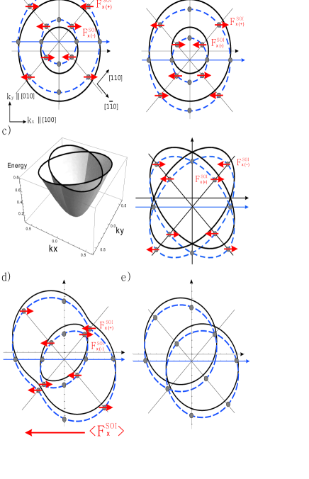
Figure 1: (Color online) The transverse SOIF vector ($F^{SOI}_{x(n)}=-qn\frac{\partial\Delta}{\partial k_{x}\partial k_{y}}|E_{y}|$) distribution. The arrow (red) represents the transverse SOIF vector, and the dashed line (blue) represents the deviation in the energy band due to the electric field applied in the +y direction ([010] direction). (a) hole system with isotropic dispersion; (b) electron system with isotropic dispersion; (c) 2D k-cubic Dresselhaus system; (d) Rashba and Dresselhaus system with $\alpha\neq\beta$; (e) Rashba and Dresselhaus system with $\alpha=\beta$.

The SOIF vector distribution at a 2D $k$-plane is shown in Fig. 1, where only the transverse SOIF is illustrated in the figure. The electric field is applied in the $+y$ direction (i.e., $[010]$ direction), and thus, the energy dispersion would be displaced toward $+y$ direction in hole system and toward $-y$ direction in electron system. $F^{SOI}_{x(n)}=-qn\frac{\partial\Delta}{\partial k_{x}\partial k_{y}}|E_{y}|$ represents the transverse SOIF of the $n$-th band. The SOIF vector distribution in the hole isotropic system is given in (a) and that in the electron system is given in (b). The transverse SOIF vector of the 2D k-cubic Dresselhaus system is shown in Fig. 1. (c). At the angles $0$, $\frac{\pi}{2}$, $\pi$, and $\frac{3\pi}{2}$, the SOIF vanishes in the isotropic and anisotropic systems. We note that in the isotropic system, the electron (hole) concentration in the $k$-plane is symmetric along the $y$-axis, and the mean transverse SOIF is zero. This implies that the applied electric field would not result in the charge imbalance at the edges of the sample. In the Rashba-Dresselhaus system ((d) in Fig. 1.), the electron concentrations on the left-hand and right-hand sides of the $k$-plane are equal. However, the mean transverse SOIF does not vanish (see the following section). In this system, the non-vanishing mean transverse SOIF acts as the driving force and results in charge imbalance at the edges of the sample. This implies that a non-zero Hall voltage can be detected in the Rashba-dresselhaus system when only an electric field is present. This is rather different from the classical charge Hall effect, where an external magnetic field must be applied to the system.

IV Rashba-Dresselhaus system

In this section, we study the mean SOIF in the Rashba-Dresselhaus system. The Hamiltonian can be written as $H_{0}=\frac{\hbar^{2}k^{2}}{2m}+\alpha(\sigma_{x}k_{y}-\sigma_{y}k_{x})-\beta(\sigma_{x}k_{x}-\sigma_{y}k_{y})$. The energy dispersion is $E_{nk}=\frac{\hbar^{2}k^{2}}{2m}-n\Delta(\mathbf{k})$, where $\Delta(\mathbf{k})=\sqrt{(\alpha^{2}+\beta^{2})k^{2}-4\alpha\beta k_{x}k_{y}}=k\gamma(\phi)$, and $\gamma(\phi)=\sqrt{\alpha^{2}+\beta^{2}-2\alpha\beta\sin(2\phi)}$. In our notation, $\Delta_{n}(\mathbf{k})=-n\Delta$ and $h_{so}=\alpha(\sigma_{x}k_{y}-\sigma_{y}k_{x})-\beta(\sigma_{x}k_{x}-\sigma_{y}k_{y})$.

IV.1 Non-vanishing longitudinal and transverse SOIF

In the Rashba-Dresselhaus system, the longitudinal coefficient $K_{yy}$ can be evaluated analytically:

$$K_{yy}=-\frac{m^{2}}{2\pi\hbar^{4}}|\alpha^{2}-\beta^{2}|.$$ (23)

We note that $K_{yy}$ is always negative in the Rashba-Dresselhaus system when $\alpha\neq\beta$. This means that the longitudinal SOIF acts in a direction opposite to that of Lorentz force. The longitudinal coefficient $K_{yy}$ is approximately $10^{-7}(1/$Å${}^{2})$ in semiconductor with large built-in electric field ($\alpha\sim 10^{-2}$eVÅ) Cho05 , which is very small in comparison with the value of the Lorentz force (free carrier density is approximately $10^{-4}(1/$Å${}^{2})$ in the Rashba-Dresselhaus system, see Ref. Gan06 ). The mean longitudinal SOIF is non-zero in the Rashba system ($\beta=0$) as well as in the Dresselhaus system ($\alpha=0$). On the other hand, the integrand of the off-diagonal component of $K_{ij}$ (transverse coefficient) is $\frac{\partial^{2}\Delta}{\partial k_{x}\partial k_{y}}=-\frac{(\alpha^{2}-\beta^{2})^{2}}{\Delta^{3}}k_{x}k_{y}$. The transverse coefficient $K_{xy}$ can be evaluated analytically. We find that $K_{xy}$ also depends on the Rashba and Dresselhaus couplings, and in general, it does not vanish if $\alpha\neq\beta$:

$$\begin{split}K_{xy}&=-\frac{m}{4\pi^{2}\hbar^{2}}\int^{k_{+}}_{k_{-}}dS_{k}\frac{\partial^{2}\Delta}{\partial k_{x}\partial k_{y}}\\ &=\frac{m^{2}}{2\pi\hbar^{4}}\left\{\begin{array}[]{cc}\displaystyle{\frac{\beta}{\alpha}|\alpha^{2}-\beta^{2}|}&~{};~{}\alpha^{2}>\beta^{2}\\ \\ \displaystyle{\frac{\alpha}{\beta}|\alpha^{2}-\beta^{2}|}&~{};~{}\beta^{2}>\alpha^{2}\end{array}\right..\end{split}$$ (24)

Therefore, the system has a net SOIF in the -x direction, namely, $\langle F_{x}^{SOI}\rangle=-|e|K_{xy}E_{y}$ and $K_{xy}>0$ (see Fig.1 (d)). When the Rashba coupling is equal to the Dresselhaus coupling, the transverse SOIF vanishes, and further the energy dispersion is not isotropic ($\Delta(\alpha=\beta)=\sqrt{2}\alpha|k_{x}-k_{y}|$; see Fig. 1. (e)).

In the Rashba-Dresselhaus system, we have $\partial^{2}h_{so}/\partial k_{i}\partial k_{j}=0$, and the relation in Eq. (22) follows. This can be examined by the direct calculation of the conventional spin Hall conductivity. The force $F_{x}^{O}=\frac{4m^{2}}{\hbar^{4}}(\alpha^{2}-\beta^{2})(\mathbf{J}^{s_{z}}\times\hat{e}_{z})_{x}=\frac{4m^{2}}{\hbar^{4}}(\alpha^{2}-\beta^{2})J_{y}^{s_{z}}$ is shown to be proportional to the conventional spin longitudinal conductivity $\sigma^{s}_{yy}$ Shen05 . It can be shown that $\sigma^{s}_{yy}=\frac{q}{8\pi^{2}}(\alpha^{2}-\beta^{2})\int_{0}^{2\pi}d\phi\frac{\sin\phi\cos\phi}{\gamma(\phi)^{2}}$. We have $\sigma^{s}_{yy}=\frac{q}{8\pi}\frac{\beta}{\alpha}$ for $\alpha^{2}>\beta^{2}$ and $\sigma^{s}_{yy}=-\frac{q}{8\pi}\frac{\alpha}{\beta}$ for $\beta^{2}>\alpha^{2}$. We obtain $\langle F_{x}^{O}\rangle=\frac{qm^{2}}{2\pi\hbar^{4}}\frac{\beta}{\alpha}(\alpha^{2}-\beta^{2})E_{y}$ for $\alpha^{2}>\beta^{2}$ and $\langle F_{x}^{O}\rangle=\frac{qm^{2}}{2\pi\hbar^{4}}\frac{\alpha}{\beta}(\beta^{2}-\alpha^{2})E_{y}$ for $\beta^{2}>\alpha^{2}$; this is in agreement with the result of Eq. (24). Therefore, physically the linear response of $\mathbf{F}^{O}$ to the weak electric field is identical to the semiclassical force acting on a band electron in this case. Due to the non-vanishing transverse force in the Rashba-Dresselhaus system, the charge imbalance would exist in the system even in the absence of an external magnetic field because the mean transverse SOIF acts as the driving force.

On the other hand, when an electric field is applied in the $[\bar{1}10]$ direction denoted as $k_{y}^{\prime}$ direction, the effective Hamiltonian can be rewritten as $H^{\prime}_{0}=\frac{\hbar^{2}k^{\prime 2}}{2m}+\frac{1}{\sqrt{2}}(\sigma_{x}-\sigma_{y})(\alpha-\beta)k_{x}^{\prime}+\frac{1}{\sqrt{2}}(\sigma_{x}+\sigma_{y})(\alpha+\beta)k_{y}^{\prime}$, where the energy dispersion is $\gamma^{\prime}(\phi)=\sqrt{(\alpha-\beta)^{2}\cos^{2}\phi+(\alpha+\beta)^{2}\sin^{2}\phi}$. In this case, it can be shown that $K_{x^{\prime}y^{\prime}}$ integral vanishes. It is interesting to note that the conventional spin-Hall conductivity in this case is not an universal constant Sinova04 . We find that the conventional spin-Hall conductivity depends on the strength of spin-orbit coupling: $\sigma^{z}_{x^{\prime}y^{\prime}}=\frac{q}{8\pi}(1+\frac{\beta}{\alpha})$, $\alpha>\beta$ and $\sigma^{z}_{x^{\prime}y^{\prime}}=-\frac{q}{8\pi}(1+\frac{\alpha}{\beta})$, $\alpha<\beta$. Furthermore, we find that $\sigma^{z}_{y^{\prime}x^{\prime}}=-\frac{q}{8\pi}(1-\frac{\beta}{\alpha})$, $\alpha>\beta$ and $\sigma^{z}_{y^{\prime}x^{\prime}}=\frac{q}{8\pi}(1-\frac{\alpha}{\beta})$, $\beta>\alpha$, from which we have an unsymmetrical result $\sigma^{z}_{x^{\prime}y^{\prime}}\neq-\sigma^{z}_{y^{\prime}x^{\prime}}$. This is because $[110]$ and $[1\bar{1}0]$ are nonequivalent axes in the sense that the Rashba-Dresselhaus system has the $C_{2v}$ symmetry Wink03 . The resulting spin splittings along the $[110]$ and $[1\bar{1}0]$ directions are equal to $2(\alpha+\beta)k^{\prime}$ and $2(\alpha-\beta)k^{\prime}$, respectively.

IV.2 The Hall voltage

When an external in-plane electric field is applied to the Rashba-Dresselhaus system, the charge accumulation generated by the spin Hall current does not result in charge imbalance because the system has equal populations of electrons with $+z$ and $-z$ polarized spins. However, as shown in the above subsection, we find that the mean transverse SOIF which is independent of spin components does not vanish in the Rashba-Dresselhaus system. As a result, the existence of the non-zero transverse force leads to a charge imbalance between two edges of the sample. Furthermore, we can estimate the resulting Hall voltage from the classical point of view. When the system reaches an equilibrium, the transverse electric field generated by the charge imbalance can balance the mean single-particle transverse SOIF which is defined as

$$\langle\langle F^{SOI}_{x}\rangle\rangle=\frac{\langle F^{SOI}_{x}\rangle}{n_{c}},$$ (25)

where $n_{c}=\frac{1}{4\pi}\left[\frac{4m\epsilon_{F}}{\hbar^{2}}+(\frac{2m}{\hbar^{2}})^{2}(\alpha^{2}+\beta^{2})\right]$ is the electron concentration. Therefore, an equilibrium state requires $\langle\langle F^{SOI}_{x}\rangle\rangle=qE_{x}=q\frac{V_{H}}{W}$, where $V_{H}$ is the Hall voltage, and $W$ is the width of a device. On the other hand, $\langle\langle F^{SOI}_{x}\rangle\rangle=(K_{xy}/n_{c})qE_{y}=(K_{xy}/n_{c})q\frac{V_{L}}{L}$, where $V_{L}$ is the longitudinal voltage and $L$ is the length of a device. Therefore, the Hall voltage can be written as

$$V_{H}=\frac{K_{xy}}{n_{c}}\frac{W}{L}V_{L}.$$ (26)

Unlike the classical charge-Hall effect, the non-zero Hall voltage occurs in the absence of an external magnetic field. Figure 2(a) shows $\frac{K_{xy}}{n_{c}}$ as a function of the Rashba coupling, where the Dresselhaus coupling is fixed to $\beta=7.5\times 10^{-4}eV\AA$. As shown in Fig. 2(a), the maximum value of $K_{xy}/n_{c}$ for the Fermi energy being smaller than $10^{-5}$ is about $10^{-2}$. We assume that the length-to-width ratio is equal to 8 and the longitudinal voltage is about $10^{-3}$ (Volt) Kli80 . We find that the Hall voltage is nearly equal to $1\mu V$.

Figure 1(d) shows the direction of the transverse SOIF vector in different k points. If the mean transverse SOIF in $-x$ direction is denoted as a minus sign and that in $+x$ direction is denoted as plus sign, then the populations of electrons corresponding to those different directions of the mean SOIF is illustrated in the inset of Fig. 2(b). We define a deviation of electron concentration as

$$\delta n=n_{+}-n_{-},$$ (27)

where $n_{+}$ and $n_{-}$ refer to the electron concentration with the transverse SOIF vector in $+x$ and $-x$ directions, respectively. In other words, $n_{-}$ is the sum over all shaded regions shown in the inset of Fig. 2(b), and the sum over all unshaded regions gives $n_{+}$. Each region ranges from zero to the corresponding wave vector, and it follows that

$$\begin{split}n_{+}&=\frac{1}{(2\pi)^{2}}\left(\int_{0}^{\pi/2}k_{-}^{2}(\phi)d\phi+\int^{\pi}_{\pi/2}k_{+}^{2}(\phi)d\phi\right)\\ n_{-}&=\frac{1}{(2\pi)^{2}}\left(\int_{0}^{\pi/2}k_{+}^{2}(\phi)d\phi+\int^{\pi}_{\pi/2}k_{-}^{2}(\phi)d\phi\right),\end{split}$$ (28)

where $k_{\pm}(\phi)=\pm\frac{m}{\hbar^{2}}\gamma(\phi)+\left((\frac{m}{\hbar^{2}})^{2}\gamma(\phi)^{2}+\frac{2m\epsilon_{F}}{\hbar^{2}}\right)^{1/2}$.

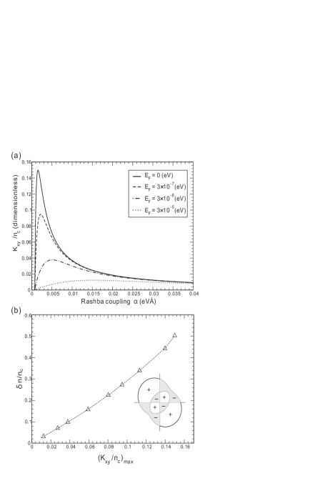
Figure 2: (a) The dimensionless quantity $K_{xy}/n_{c}$ as a function of the Rashba coupling; (b) The deviation of the electron concentration $\delta n/n_{c}$ varies with respect to the maximum value of $K_{xy}/n_{c}$.

Equation (27) is interesting because it is the origin of charge imbalance that requires the population of electrons at two edges of the sample to be different. In this case, we find that the deviation $\delta n/n_{c}$ grows as the maximum value of $K_{xy}/n_{c}$ denoted as $(K_{xy}/n_{c})_{max}$ increases (see Fig. 2(b)). This result explains that the charge imbalance can be characterized through the calculation of $K_{xy}$ and clarifies the significance of our expression for the mean transverse SOIF. Quantitatively, the calculation of $K_{ij}$ [Eq. (19)] is important because the charge imbalance cannot reach to the value $\delta n$, and thus, the resulting Hall voltage cannot be determined from $\delta n$.

We close this subsection by some discussions on gauge transformation and the charge Hall current. By using Eqs. (11) and (12), the charge current $J_{i}=qv_{i}$ in the ballistic region can be written as MCChang05

$$\langle J_{i}\rangle=\frac{q^{2}}{\hbar\mathcal{V}}\sum_{\mathbf{k}n}f_{n\mathbf{k}}\mathcal{F}^{(n)}_{ij}E_{j},$$ (29)

where

$$\mathcal{F}^{(n)}_{ij}=\frac{\partial A^{(n)}_{j}}{\partial k_{i}}-\frac{\partial A^{(n)}_{i}}{\partial k_{j}}$$ (30)

is the field strength of $n$-th band in $k$-space, and it satisfies the antisymmetric property $\mathcal{F}^{(n)}_{ij}=-\mathcal{F}^{(n)}_{ji}$. The Berry vector potential in Eq. (30) is defined as $A^{(n)}_{i}=\langle n\mathbf{k}|(-i)\frac{\partial}{\partial k_{i}}|n\mathbf{k}\rangle$. We note that the longitudinal charge current always vanishes, as shown in Eq. (30), where the anti-symmetric property of $\mathcal{F}^{(n)}_{ij}$ guarantees that $\mathcal{F}^{(n)}_{ii}$ is zero, and this result is independent of any gauge choice. Physically, this means that there is no steady longitudinal current without considering the collision with impurity. In that sense, the existence of a steady charge-Hall current generated by the spin Hall effect is possible because there is no transverse electric field. However, the charge Hall current can not be uniquely determined from Eq. (29) because the singular gauge transformation changes the magnitude of the charge Hall conductivity in 2D spin-orbit coupled systems MCChang05 . On the other hand, the system has equal populations of electrons with $+z$ and $-z$ polarized spins. Therefore, in Ref. MCChang05 , a specific gauge is chosen such that the steady charge-Hall current is zero.

Nevertheless, the mean transverse SOIF does not vanishes in the ballistic region, and thus, the non-steady charge Hall current exists in the Rashba-Dresselhaus system. As a result, the charge imbalance between two edges of the sample can occur in the system. The system can still have an equilibrium state in the sense that the transverse electric field generated by charge imbalance can balance the mean single-particle transverse SOIF.

IV.3 Disorder effect

In this section, we will consider the weak disorder effect. We will show that the transverse SOIF vanishes if the calculation is carried out to the order of $\frac{\Delta_{F}}{\epsilon_{F}}$ in the sense that the Fermi energy ($\epsilon_{F}\equiv\hbar^{2}k_{F}^{2}/2m$) is much larger than the spin-splitting ($\Delta_{F}=2\gamma(\phi)k_{F}$). In the Rashba-Dresselhaus system, the transverse force is determined by $\mathbf{F}^{O}$ because $\mathbf{F}^{E}=0$. It can be represented by the term proportional to spin current $J^{z}_{y}=\frac{1}{2}\{v_{y},s_{z}\}$, i.e., $F_{x}^{O}=\frac{4m^{2}}{\hbar^{4}}(\alpha^{2}-\beta^{2})J^{z}_{y}$. Therefore the calculation of force is simplified to the calculation of conventional spin-Hall conductivity. Because $F_{x}^{O}$ is proportional to $J_{y}^{z}$, we have to calculate the spin-longitudinal conductivity $\sigma^{s_{z}}_{yy}$.

The impurity is assumed to have a $\delta$-potential $V(\mathbf{x})=V_{0}\mathbf{1}\sum_{i}\delta(\mathbf{x}-\mathbf{R}_{i})$, where $\mathbf{R}_{i}$ is the location of the $i$-th impurity and $V_{0}$ is the potential strength. The relaxation time $\tau$ can be obtained from the calculation of the self-energy by using the definition $\frac{\hbar}{\tau}=2|Im\Sigma|$. For the impurity potential $V(\mathbf{x})=V_{0}\mathbf{1}\sum_{i}\delta(\mathbf{x}-\mathbf{R}_{i})$, the self-energy can be calculated by the the following equation Dug05 : $\Sigma(\epsilon)=\frac{\langle n_{i}V_{0}^{2}\rangle}{2}\sum_{s}\int d\mathbf{k}G_{k,s}(\epsilon)$, where $G_{k,s}(\epsilon)=1/[\epsilon-\epsilon_{ks}-\Sigma(\epsilon)]$, and $n_{i}$ is the impurity concentration. In the Born approximation Dug05 ,

$$\frac{\hbar}{\tau}=\pi\langle n_{i}V_{0}^{2}\rangle(N_{+}+N_{-}),$$ (31)

where $N_{s}$ is the density of states of band $s$. In the Rashba-Dresselhaus system, the total density of states is $(N_{+}+N_{-})=\frac{1}{2\pi}(k_{+}\frac{dk_{+}}{d\epsilon_{F}}+k_{-}\frac{dk_{-}}{d\epsilon_{F}})=\frac{m}{\pi\hbar^{2}}$, and thus, $\langle n_{i}V_{0}^{2}\rangle=\frac{\hbar^{3}}{m\tau}$. The retarded and advanced Green’s functions are diagonal in the helicity space, that is,

$$G^{R,A}(\epsilon)=\left(\begin{array}[]{cc}G^{R,A}_{+}(\epsilon)&0\\ 0&G^{R,A}_{-}(\epsilon)\\ \end{array}\right),$$ (32)

where

$$G^{R}_{s}(\epsilon) =\frac{1}{\epsilon-\epsilon_{ks}+i\Gamma}~{};$$ (33a)

$$G^{A}_{s}(\epsilon) =\frac{1}{\epsilon-\epsilon_{ks}-i\Gamma}.$$ (33b)

$\Gamma$ is defined as $\Gamma=\frac{\hbar}{2\tau}$. The spin longitudinal conductivity $\sigma^{s_{z}}_{yy}$ can be evaluated by calculating the following Green’s function Arii07 :

$$\Theta^{RA}(\epsilon,\epsilon^{\prime})=\frac{q\hbar}{2\pi}\int d\mathbf{k}Tr[J_{y}^{z}G^{R}(\epsilon)\mathcal{V}_{y}G^{A}(\epsilon^{\prime})],$$ (34)

where $\epsilon^{\prime}=\epsilon-\hbar\omega$ and $\mathcal{V}_{y}$ includes the vertex correction [see Eq. (36)]. The notation $Tr$ represents the trace in the helicity space $s$. Here, the electric field is applied in the y-direction, and we calculate the spin current in the y direction, which has a spin component in the z direction. The spin longitudinal conductivity $\sigma^{s_{z}}_{yy}$ can be evaluated by using the formula Arii07

$$\sigma^{s_{z}}_{yy}=-\int d\epsilon\frac{f(\epsilon-\hbar\omega)-f(\epsilon)}{\hbar\omega}\Theta^{RA}(\epsilon,\epsilon-\hbar\omega),$$ (35)

where $f(\epsilon)$ is the Fermi-Dirac distribution. In the ladder approximation, the vertex correction of electric velocity $\mathcal{V}_{x}$ satisfies the self-consistent vertex equation Arii07 :

$$\mathcal{V}_{y}=v_{y}+\langle n_{i}V_{0}^{2}\rangle\int\frac{d\mathbf{k}}{(2\pi)^{2}}G^{R}\mathcal{V}_{y}G^{A}.$$ (36)

The electron velocity $\mathcal{V}_{y}$ can be divided into two parts, $\mathcal{V}_{y}=v_{y}+\tilde{v}_{y}$, where $v_{y}$ is the electron velocity in the absence of impurities and $\tilde{v}_{y}$ is the vertex correction in the presence of impurities. The vertex correction of velocity, $\tilde{v}_{y}$, can be written as $\tilde{v}_{y}=\sum_{\mu=0}^{3}c_{\mu}\sigma_{\mu}$ (See also Eq. (37)), and the general solution of Eq. (36) is given by zhou07

$$\mathcal{V}_{y}=v_{y}+\sum_{\mu}\sigma_{\mu}c_{\mu}~{};~{}\mu=0,1,2,3,.$$ (37)

The matrix $\sigma_{0}$ is the two by two identity matrix, and $\sigma_{i}$ ($i=1,2,3$ corresponds to $x,y,z$) are the Pauli matrices. We substitute Eq. (37) into Eq. (36) and obtain the matrix equation

$$\sum_{\nu}Q_{\mu\nu}c_{\nu}=D_{\mu}~{};~{}\mu,\nu=0,1,2,3,$$ (38)

where

$$Q_{\mu\nu}=2\delta_{\mu\nu}-\langle n_{i}V_{0}^{2}\rangle\int\frac{d\mathbf{k}}{(2\pi)^{2}}Tr[G^{R}\sigma_{\nu}G^{A}\sigma_{\mu}],$$ (39)

where it can be shown that $Q_{30}=Q_{03}=0$ and

$$D_{\mu}=\langle n_{i}V_{0}^{2}\rangle\int\frac{d\mathbf{k}}{(2\pi)^{2}}Tr[G^{R}v_{y}G^{A}\sigma_{\mu}].$$ (40)

It can be shown that $Q_{13}$, $Q_{23}$ (and thus $Q_{31}$ and $Q_{32}$), and $D_{3}$ represent purely interband transitions. If we assume that the scattering effect does not cause any interband transition (i.e. this assumption is equivalent to $\Delta_{F}>>\hbar\omega$), we can neglect these terms in the calculation. Then in this case, the coefficient $c_{z}$ is zero. On the other hand, if we restrict each $Q_{ij}$ and $D_{j}$ to the order of $\Delta_{F}/\epsilon_{F}$, we can neglect $Q_{01}$, $Q_{02}$ (as well as $Q_{10}$ and $Q_{20}$), and $D_{0}$ from which we can conclude that $c_{0}=0$. Therefore, Eq. (38) simplifies to the following two by two matrix equation:

$$\left(\begin{array}[]{cc}Q_{11}&Q_{12}\\ Q_{21}&Q_{22}\end{array}\right)\left(\begin{array}[]{c}c_{x}\\ c_{y}\end{array}\right)=\left(\begin{array}[]{c}D_{1}\\ D_{2}\end{array}\right).$$ (41)

In the DC limit $\omega\rightarrow 0$ (taken before the limit $\tau\rightarrow\infty$), we obtain $D_{1}=\frac{\alpha}{\hbar}(f_{1}-2)-\frac{\beta}{\hbar}f_{2}$, $D_{2}=-\frac{\alpha}{\hbar}f_{2}+\frac{\beta}{\hbar}(f_{3}-2)$, $Q_{11}=2-f_{1}$, $Q_{22}=2-f_{3}$, and $Q_{12}=Q_{21}=f_{2}$, where $f_{i}$ $(i=1,2,3)$ are the following integrals:

$$\begin{split}f_{1}&=\frac{1}{\pi}\int_{0}^{2\pi}d\phi\frac{(\alpha\sin\phi-\beta\cos\phi)^{2}}{\gamma(\phi)^{2}},\\ f_{2}&=\frac{1}{\pi}\int_{0}^{2\pi}d\phi\frac{(\alpha\sin\phi-\beta\cos\phi)(\alpha\cos\phi-\beta\sin\phi)}{\gamma(\phi)^{2}},\\ f_{3}&=\frac{1}{\pi}\int_{0}^{2\pi}d\phi\frac{(\alpha\cos\phi-\beta\sin\phi)^{2}}{\gamma(\phi)^{2}};\end{split}$$ (42)

here, $\gamma(\phi)=\sqrt{\alpha^{2}+\beta^{2}-2\alpha\beta\sin(2\phi)}$. After integration, we have $f_{1}=f_{3}=1$ and $f_{2}=-\frac{\beta}{\alpha}$ for $\alpha>\beta$, and $f_{2}=-\frac{\alpha}{\beta}$ for $\alpha<\beta$. Substituting $f_{1}$, $f_{2}$, and $f_{3}$ into Eq. (41), we obtain $c_{x}$ and $c_{y}$:

$$\left(\begin{array}[]{c}c_{x}(\omega=0)\\ c_{y}(\omega=0)\end{array}\right)=\left(\begin{array}[]{c}-\alpha/\hbar\\ -\beta/\hbar\end{array}\right)~{};~{}\alpha\neq\beta.$$ (43)

However, we have $\mathcal{V}_{y}=v_{y}+c_{x}\sigma_{x}+c_{y}\sigma_{y}=v_{y}^{0}+(c_{x}+\frac{\alpha}{\hbar})\sigma_{x}+(c_{y}+\frac{\beta}{\hbar})\sigma_{y}$, where $v^{0}_{y}=\hbar k_{y}/m$. Therefore, the vertex correction cancels the anomalous velocity $\frac{\alpha}{\hbar}\sigma_{x}+\frac{\beta}{\hbar}\sigma_{y}$. Finally, the spin longitudinal conductivity $\sigma^{s_{z}}_{yy}$ is proportional to the term $v_{y}^{0}v_{y}^{0}Tr[\sigma_{z}G^{R}G^{A}]=v_{y}^{0}v_{y}^{0}Tr[\sigma_{z}G^{R}\sigma_{0}G^{A}]$. It can be shown that the trace directly equals zero, that is, $Tr[\sigma_{z}G^{R}\sigma_{0}G^{A}]=0$, and thus, the spin longitudinal conductivity is zero. This implies that the transverse force in the Rashba-Dresselhaus system vanishes when the disorder effect is considered. In the same approximation, the spin-Hall conductivity also vanishes. This can be seen as follows. The spin-Hall current is proportional to $k_{x}\sigma_{z}$, and the spin Hall conductivity $\sigma^{x}_{xy}$ is proportional to the term $v^{0}_{y}v^{0}_{x}Tr[\sigma_{z}G^{R}\sigma_{0}G^{A}]$ in which the trace term is the same as the spin longitudinal conductivity, and thus, we obtain the vanishing spin-Hall conductivity. The result obtained from Eq. (43) agrees with the expected result for the pure Rashba system Mish04 ; Cha05 ; Bry06 ; Arii07 ; zhou07 and pure Dresselhaus system Malshu05 . The influence of impurities on spin-Hall transport in the Rashba and Dresselhaus system also has been studied in Refs. Loss03 and syn04 by means of Boltzmann equation and Kubo formula, respectively. However, the vertex correction [Eq. (36)] which is non-zero in the diffusive regime Cha05 ; Bry06 is not taken into account in both calculations.

In short, Eq. (20) is valid in any spin-orbit coupled system with the Hamiltonian given by Eq. (1). The charge imbalance would occur in the Rashba-Dresselhaus system in the clean limit when the the electric field is applied in the system. However, it is shown that the disorder can cancel the transverse force, and thus, the charge imbalance would not occur in this case.

V Conclusions

In conclusion, we show that the mean SOIF (spin-orbit interaction induced force, Eq. (18)) in any spin-orbit coupled systems is determined by the second derivative of energy dispersion [Eq. (19)] only. The mean transverse SOIF acts as the driving force and thus results in transverse charge imbalance in the spin-orbit coupled system. It has been shown that the mean transverse SOIF vanishes in rotationally invariant systems such as Luttinger, k-linear Rashba, k-cubic Rashba, k-linear Dresselhaus, and wurtzite systems. Furthermore, we find that the mean SOIF also vanishes in the 2D k-cubic Dresselhaus system, where the energy dispersion is anisotropic. Nonetheless, we find that the mean transverse SOIF does not vanish in the Rashba-Dresselhaus system. This result can be verified by measuring the Hall voltage in the absence of an external magnetic field. The estimated magnitude of Hall voltage is nearly equal to $1\mu$V when a longitudinal voltage of 1meV is applied. In the presence of weak disorder, the SOIF vanishes in the Rashba-Dresselhaus system because the anomalous velocity and vertex correction accidently cancel each other.

The electrical measurement of intrinsic spin-Hall effect in the ballistic region has recently been carried out for HgTe nanostructures Bru08 . Therefore, we believe that the transverse charge imbalance resulting from the non-zero transverse SOIF can be detected in the ballistic region by measuring the Hall voltage. Hopefully, our interesting prediction would stimulate measurements of the Hall voltage in such spin-orbit coupled systems with an anisotropic dispersion as the Rashba-Dresselhaus system in the near future.

References

- (1) J. D. Jackson, Classical Electrodynamics (New York: Wiley, 1999 3rd ed).
- (2) N. W. Ashcroft and N. D. Mermin, Solid State Physics (New York: Rinehart and Winston, 1976); W. A. Harrison, Solid State Theory (Dover, 1980).
- (3) C.-M. Ryu, Phys. Rev. Lett. 76, 968 (1996).
- (4) M. C. Chang and Q. Niu, Phys. Rev. Lett. 75, 1348 (1995); Phys. Rev. B 53, 7010 (1996); G. Sundaram and Q. Niu, Phys. Rev. B 59, 14915 (1999).
- (5) M. C. Chang and Q. Niu, J. Phys.: Condens. Matter, 20, 193202 (2008).
- (6) H. Koizumi and Y. Takada, Phys. Rev. B 65, 153104 (2002).
- (7) S. Murakami, N. Nagaosa, and S.-C. Zhang, Science 301, 1348 (2003); Phys. Rev. B 69, 235206 (2004).
- (8) Z. Fang, N. Nagaosa, K. S. Takahashi, A. Asamitsu, R. Mathieu, T. Ogasawara, H. Yamada, M. Kawasaki, Y. Tokura, and K. Terakura, Science 302, 92 (2003).
- (9) G. Y. Guo, Y. Yao, and Q. Niu, Phys. Rev. Lett. 94, 226601 (2005).
- (10) G. Y. Guo, S. Murakami, T.-W. Chen, and N. Nagaosa, Phys. Rev. Lett. 100, 096401 (2008).
- (11) B. K. Nikolić, L. P. Zârbo, and S. Welack, Phys. Rev. B 72, 075335 (2005).
- (12) S.-Q. Shen, Phys. Rev. Lett. 95, 187203 (2005); K. Y. Bliokh, Europhys. Lett. 72, 7 (2005); W. Zawadzki, Phys. Rev. Lett. 99, 179701 (2007).
- (13) P.-Q. Jin, Y.-Q. Li, and F.-C. Zhang, J. Phys. A: Math. Gen. 39, 7115 (2006).
- (14) J. Shibata and H. Kohno, Phys. Rev. Lett. 102, 086603 (2009).
- (15) T.-W. Chen and G. Y. Guo, Phys. Rev. B 79, 125301 (2009).
- (16) T.-W. Chen, C. M. Huang, and G. Y. Guo, Phys. Rev. B 73, 235309 (2006).
- (17) B. Zhou, L. Ren, S.-Q. Shen. Phys. Rev. B 73, 165303 (2006).
- (18) J. B. Miller, D. M. Zumbuhl, C. M. Marcus, Y. B. Lyanda-Geller, D. Goldhaber-Gordon, K. Campman, and A. C. Gossard, Phys. Rev. Lett. 90, 076807 (2003); A. G. Mal’shukov and K. A. Chao, Phys. Rev. B 71, 121308(R) (2005).
- (19) J. Cserti and G. David, Phys. Rev. B 74, 172305 (2006).
- (20) Y. A. Bychkov and E. I. Rashba, J. Phys. C 17, 6039 (1984).
- (21) G. Dresselhaus, Phys. Rev. 100, 580 (1955).
- (22) R. Winkler, Phys. Rev. B 62, 4245 (2000).
- (23) I. Zorkani and E. Kartheuser, Phys. Rev. B 53, 1871 (1996).
- (24) I. Žutić, J. Fabian and D. Sarma, Rev. Mod. Phys. 76, 323 (2004).
- (25) K. S. Cho, T. Y. Huang, H. S. Wang, M. G. Lin, T. M. Chen, C. T. Liang, and Y. F. Chen, Appl. Phys. Lett. 86, 222102 (2005); H. J. Chang, T. W. Chen, J. W. Chen, W. C. Hong, W. C. Tsai, Y. F. Chen, and G. Y. Guo, Phys. Rev. Lett. 98, 136403 (2007).
- (26) S. D. Ganichev, V. V. Belkov, L. E. Golub, E. L. Ivchenko, Petra Schneider, S. Giglberger, J. Eroms, J. De Boeck, G. Borghs, W. Wegscheider, D. Weiss, and W. Prettl, Phys. Rev. Lett. 92, 256601 (2004).
- (27) J. Sinova, D. Culcer, Q. Niu, N. A. Sinitsyn, T. Jungwirth, and A. H. MacDonald, Phys. Rev. Lett. 92 126603 (2004).
- (28) R. Winkler, Spin-Orbit Coupling Effects in Two-Dimensional Electron and Hole System (Springer, 2003).
- (29) K. v. Klitzing, G. Dorda, and M. Pepper, Phys. Rev. Lett. 45, 494 (1980).
- (30) M. C. Chang, Phys. Rev. B 71, 085315 (2005).
- (31) V. K. Dugaev, P. Bruno, M. Taillefumier, B. Canals, and C. Lacroix, Phys. Rev. B 71, 224423 (2005).
- (32) K. Arii, M. Koshino, and T. Ando, Phys. Rev. B 76, 045311 (2007).
- (33) B. Zhou, C.-X. Liu, and S.-Q. Shen, Europhys. Lett. 79, 47010 (2007).
- (34) E. G. Mishchenko, A. V. Shytov, and B. I. Halperin, Phys. Rev. Lett. 93, 226602 (2004); O. V. Dimitrova, Phys. Rev. B 71, 245327 (2005); N. Sugimoto, S. Onoda, S. Murakami, and N. Nagaosa, Phys. Rev. B 73, 113305 (2006).
- (35) J. I. Inoue, G. E. W. Bauer, and L. W. Molenkamp, Phys. Rev. B 70, 041303(R) (2004); R. Raimondi and P. Schwab, Phys. Rev. B 71, 033311 (2005); O. Chalaev and D. Loss, Phys. Rev. B 71, 245318 (2005).
- (36) V. V. Bryksin and P. Kleinert, Phys. Rev. B 73, 165313 (2006).
- (37) J. Schliemann and D. Loss, Phys. Rev. B 68, 165311 (2003).
- (38) N. A. Sinitsyn, E. M. Hankiewicz, W. Teizer, and J. Sinova, Phys. Rev. B 70, 081312(R) (2004).
- (39) C. Bruene, A. Roth, E.G. Novik, M. Koenig, H. Buhmann, E.M. Hankiewicz, W. Hanke, J. Sinova, and L. W. Molenkamp, cond-mat/0812.3768.