Precession and Nutation in the $\eta$ Carinae binary system: Evidences from the X-ray light curve

Abstract

It is believed that $\eta$ Carinae is actually a massive binary system, with the wind-wind interaction responsible for the strong X-ray emission. Although the overall shape of the X-ray light curve can be explained by the high eccentricity of the binary orbit, other features like the asymmetry near periastron passage and the short quasi-periodic oscillations seen at those epochs, have not yet been accounted for. In this paper we explain these features assuming that the rotation axis of $\eta$ Carinae is not perpendicular to the orbital plane of the binary system. As a consequence, the companion star will face $\eta$ Carinae on the orbital plane at different latitudes for different orbital phases and, since both the mass loss rate and the wind velocity are latitude dependent, they would produce the observed asymmetries in the X-ray flux. We were able to reproduce the main features of the X-ray light curve assuming that the rotation axis of $\eta$ Carinae forms an angle of $29^{\circ}\pm 4^{\circ}$ with the axis of the binary orbit. We also explained the short quasi-periodic oscillations by assuming nutation of the rotation axis, with amplitude of about $5^{\circ}$ and period of about 22 days. The nutation parameters, as well as the precession of the apsis, with a period of about 274 years, are consistent with what is expected from the torques induced by the companion star.

1 Introduction

The intensity and spectrum of the high energy X-ray flux, and its strict periodicity, are probably the strongest evidence of the binary nature of the $\eta$ Carinae system. The 2-10 keV X-ray emission of $\eta$ Carinae is monitored by the Rossi X-Ray Timing Explorer RXTE since 1996, and the published results cover two cycles in the 5.52 year periodic light curve (Corcoran, 2005). The duration of the shallow minima, as well as the general qualitative behavior of the light curve, were similar in the two cycles. The long lasting intervals of almost stationary intensity were modulated by low amplitude quasi-periodic flares, and the large flux increase that occurred before the minima was enhanced by strong short duration flares (Ishibashi et al., 1999). Although the X-ray light curve was successfully reproduced by analytical approximations involving wind-wind collisions (Ishibashi et al., 1999; Corcoran et al., 2001) and by numerical simulations (Pittard et al., 1998; Okazaki et al., 2008), which also reproduced the high resolution spectra obtained with Chandra (Pittard & Corcoran, 2002), some features are still controversial, like the asymmetry near periastron passage, the short quasi-periodic oscillations seen at those epochs, and the difference in the phases of these oscillations between the two cycles (Okazaki et al., 2008; Parkin et al., 2009).

Besides X-rays, other observational features can be related to wind-wind collision. Abraham & Falceta-Gonçalves (2007) were able to reproduce the HeII $\lambda 4686$ line profiles and mean velocities detected close to the 2003.5 minimum by Steiner & Damineli (2004) and Martin, Davis & Koppelman (2006), assuming that they were formed in the cooling shocked material flowing along the winds contact surface. More important, to reproduce the line profiles reflected in the Homunculus polar cap (Stahl et al. 2005), they had to assume that the Homunculus axis is not perpendicular to the orbital plane.

The rotation axis of $\eta$ Carinae probably coincides with the axis of the Homunculus; the shape of the nebula and the measured latitude dependent stellar wind velocity are strong indications that the rotational velocity is close to its critical value (Smith, 2002; Dwarkadas & Owocki, 2002). A consequence of the inclination of the rotation axis relative to the axis of the orbital plane is that the secondary star faces $\eta$ Carinae at different latitudes as it moves along the orbit, and therefore, the latitude dependent velocity and mass loss rate of the primary’s wind will affect the intensity of the X-rays produced in the wind-wind collision region.

Also, the large rotational velocity of $\eta$ Carinae will affect its internal mass distribution, which will depart from spherical symmetry. The torque induced by the companion star will result in apsidal motions, as seen in other massive binary systems (e.g. see references in Claret & Giménez 1993). Finally, the inclination of the rotation axis of $\eta$ Carinae will produce nodding motions, which will further affect the strength of the wind-wind collision and the consequent X-ray intensity.

In this paper we will take all these effects into account and calculate the X-ray light curve of $\eta$ Carinae using the analytical approximation derived by Usov (1992) and the orbital parameters found by Abraham et al. (2005) and Abraham & Falceta-Gonçalves (2007). We will show that for reasonable values of the precession and nutation periods and amplitudes, it is possible to reproduce the asymmetries in the light curve close to periastron passage and the amplitudes and phases of the short quasi-periodic oscillations for the two binary cycles observed by $RXTE$.

2 The X-ray emission model

We will use the model derived by Usov (1992) to calculate, at each point of the orbit, the X-ray luminosity originated in the shock heated gas at both sides of the contact surface, which depends on the mass loss rates ($\dot{M_{p}}$ and $\dot{M_{s}}$) and wind velocities ($V_{p}$ and $V_{s}$) of the primary and secondary stars, respectively, and on the distance $D$ between them. Pittard & Stevens (2002) showed that for the $\eta$ Carinae binary system, the major contribution to the X-ray flux comes from the interaction surface of the secondary wind, because of its higher temperature so that the expression derived by Usov (1992) and valid for adiabatic shocks becomes:

$$F_{X}(\theta_{s})=\frac{1.3\times 10^{35}}{4\pi d^{2}D}\biggl{(}\frac{\dot{M_{s}}}{V_{s}}\biggl{)}^{3/2}(\dot{M_{p}}V_{p})^{1/2}e^{-\tau(\theta_{s})},$$ (1)

where $d$ is the distance to $\eta$ Carinae, taken as 2.3 kpc, and $\tau(\theta_{s})$ the optical depth for X-ray absorption; $\dot{M_{p}}$ and $\dot{M_{s}}$ are expressed in units of $10^{-5}$ and $10^{-6}$ $M_{\odot}$ yr^-1 respectively, $V_{p}$ and $V_{s}$ in units of $10^{3}$ km s^-1, and $D$ in units of $10^{13}$ cm; $\theta_{s}$ is the true anomaly, with $\theta_{s}=0$ at periastron. We will not take into account any possible cooling of the very dense shocked gas very close to periastron passage (Parkin et al., 2009).

We will assume that $\dot{M_{s}}$ and $V_{s}$ have constant values, although Parkin et al. (2009) proposed a reduced secondary wind velocity near periastron to explain the observed change in the X-ray hardness ratio. On the other hand, we will assume that $\dot{M_{p}}$ and $V_{p}$ depend on the latitude $\lambda\,(\theta_{s})$ at which the orbital plane intercepts the side of $\eta$ Carinae that faces the secondary star, and can be expressed as (Dwarkadas & Owocki, 2002):

$$\dot{M}(\lambda) = {\dot{M}(90\degr)}\bigl{[}1-\Omega^{2}\cos^{2}\lambda\bigr{]},$$ (2)

$$V(\lambda) = V(90\degr)\bigl{[}1-\Omega^{2}\cos^{2}\lambda\bigr{]}^{1/2},$$ (3)

with $\Omega=\omega/\omega_{c}$; $\omega$ is the rotation velocity and $\omega_{c}=(GM_{p}/R_{p}^{3})^{1/2}$ its critical value; $G$ is the gravitational constant, $M_{p}$ and $R_{p}$ are the mass and radius of $\eta$ Carinae, respectively. These expressions are valid when $\Omega$ is close to unity; they were already used to reproduce the observed wind velocity as a function of latitude in $\eta$ Carinae, as well as the shape of the Homunculus nebula (Smith, 2002; Dwarkadas & Owocki, 2002).

By replacing eq. (2) and (3) in (1) we obtain:

$$F_{X}(\theta_{s})=\frac{G(t)}{D}{\biggl{[}\frac{\dot{M_{p}}(\lambda)}{\dot{M_{p}}(90^{\circ})}}\biggr{]}^{1/2}\bigg{[}\frac{{V_{p}(\lambda)}}{{V_{p}(90^{\circ})}}\biggr{]}^{1/2}e^{-\tau_{p}(\theta_{s})},$$ (4)

with

$$G(t)=\frac{1.3\times 10^{35}}{4\pi d^{2}}\biggl{(}\frac{\dot{M_{s}}}{V_{s}}\biggr{)}^{3/2}\biggl{[}\dot{M_{p}}(90^{\circ})V_{p}(90^{\circ})\ \biggr{]}^{1/2}e^{\tau_{0}},$$ (5)

where we have defined $\tau(\theta_{s})=\tau_{p}(\theta_{s})+\tau_{0}(t)$; $\tau_{p}(\theta_{s})$ represents the absorption produced by the wind of $\eta$ Carinae intercepting the line of sight, and $\tau_{0}(t)$ is constant or a slowly varying, phase independent function of time, representing all other sources of absorption.

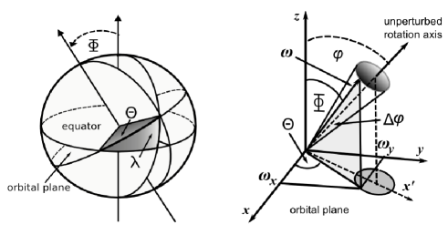
Figure 1: Left: geometrical description of the intersection of the binary system orbital plane with the surface of $\eta$ Carinae at latitude $\lambda$, $\Phi$ is the angle between the rotation axis and the perpendicular to the orbital plane; Right: definition of the different angles and coordinate systems involved in the precession of the line of apsis and nutation of the rotation axis of $\eta$ Carinae

2.1 The effects of precession and nutation on $\lambda(\theta_{s})$

$\eta$ Carinae must be highly distorted, both by rotation and by the presence of the companion star in a highly eccentric orbit. Although the total angular momentum in a detached binary system is conserved (except for a small amount lost by the stellar winds), energy will be dissipated by the tidal forces, until a minimum energy equilibrium configuration is reached, in which the orbit is circular, and the stellar spins perpendicular to the orbital plane and equal to the orbital velocity. However, although the orbital parameters are continuously changing, the orbit can be consider instantaneously Keplerian, and precession and nutation rates can be calculated as averages over the orbital period (Eggleton, Kiseleva & Hut, 1998).

In this section we will derive the effects of precession and nutation on the latitude $\lambda(\theta_{s})$. We will assume that $\eta$ Carinae rotates with angular velocity $\vec{\omega}$ around an axis that forms an angle $\Phi$ with the perpendicular to the orbital plane ($z$ axis in Figure 1), and its projection on the orbital plane forms an angle $\Theta$ with the line of apsis ($x$ axis), so that:

$$\sin\lambda(\theta_{s},t)=\sin\Theta(\theta_{s},t)\sin\Phi(t),$$ (6)

where

$$\tan\Theta\,(\theta_{s},t)=\frac{\omega_{y}}{\omega_{x}},$$ (7)

$$\sin\Phi(t)=\frac{\sqrt{\omega_{x}^{2}+\omega_{y}^{2}}}{\omega}.$$ (8)

As a consequence of nutation, the rotation angular velocity vector $\vec{\omega}$ will describe a cone of amplitude $\Delta\varphi$ and period $P_{n}$ around its non-perturbed direction, which forms an angle $\varphi$ with the polar axis $z$ (Figure 1).

In a coordinate system $(x^{\prime\prime},y^{\prime\prime},z^{\prime\prime})$, in which $z^{\prime\prime}$ is directed along the unperturbed rotation axis, the components of $\vec{\omega}$ will be $(\omega\sin\Delta\varphi\sin\omega_{n}(t)$, $\omega\sin\Delta\varphi\cos\omega_{n}(t)$, $\omega\cos\Delta\varphi)$, with $\omega_{n}(t)=(2\pi/P_{n})\Delta t+\theta_{0n}$; $\theta_{0n}$ is a constant phase and $\Delta t=t-t_{0}$, with $t_{0}=2,450,795$ being the JD of the beginning of the 1997.9 minimum. To obtain the components of $\vec{\omega}$ in the $(x,y,z)$ coordinate system, in which $z$ coincides with the orbital axis, the $(x^{\prime\prime},y^{\prime\prime},z^{\prime\prime})$ axis must be rotated around $y^{\prime\prime}$ by an angle $\varphi$, so that the new $z^{\prime}$ axis coincides with $z$, and then around $z^{\prime}$ by and angle $\theta_{s}^{\prime}=\theta_{s}+2\pi/P_{p}+\theta_{0p}$, to take into account the orbital motion and the precession of the line of apsis; $\theta_{0p}$ is a constant phase. These rotations can be represented by the matrix $M$:

$$M=\left(\begin{array}[]{ccc}\cos\theta^{\prime}_{s}&\sin\theta^{\prime}_{s}&0\\ -\sin\theta^{\prime}_{s}&\cos\theta^{\prime}_{s}&0\\ 0&0&1\end{array}\right)\left(\begin{array}[]{ccc}\cos\varphi&0&\sin\varphi\\ -\sin\varphi&0&\cos\varphi\\ 0&1&0\end{array}\right),$$ (15)

so that $(x,y,z)^{T}=M(x^{\prime\prime},y^{\prime\prime},z^{\prime\prime})^{T}$

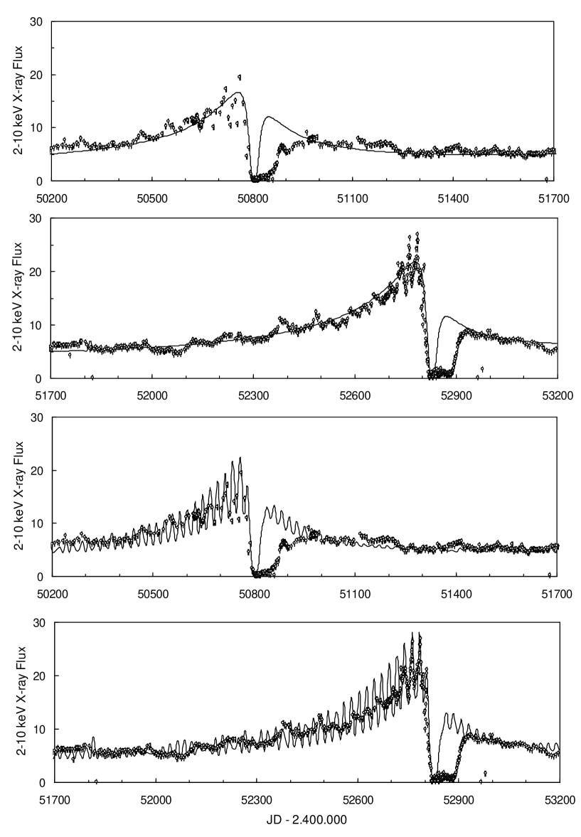
Figure 2: Observed 2-10 keV X-ray flux, from Corcoran(2005), shown as open circles, and model, shown as a continuous line, obtained with the parameters listed in Table 1, but with $\Delta\varphi=0^{\circ}$ (no nutation) in the two upper graphs and $\Delta\varphi=4\aas@@fstack{\circ}5$ for the lower ones.

2.2 Opacity and the HI column density

As mentioned before, the optical depth for X-ray absorption was divided into two parts: $\tau(\theta_{s})=\tau_{0}(t)+\tau_{p}(\theta_{s})$, where $\tau_{p}(\theta_{s})=\sigma_{\rm ph}N_{H}(\theta_{s})$ represents the photoelectric absorption produced by the unshocked wind of $\eta$ Carinae intercepting the line of sight to the vertex of the X-ray emitting cone, with column density $N_{H}$, and $\tau_{0}(t)$ that represents all other sources of absorption, excluding the stellar wind; $\sigma_{\rm ph}$ is the cross section of photoelectric absorption, multiplied by the heavy element abundance relative to H. $N_{H}(\theta_{s})$ is calculated from:

$$N_{H}(\theta_{s})=\frac{1}{4\pi\mu m_{H}}\biggl{(}\frac{\overline{\dot{M}_{p}}}{\overline{V_{p}}}\biggr{)}\int^{\infty}_{s_{\rm sh}}\frac{ds}{s^{2}+r_{0}^{2}},$$ (16)

where $\mu$ is the molecular weight and $m_{H}$ the mass of the hydrogen atom, $\overline{\dot{M}_{p}}$ and $\overline{V_{p}}$ are the mean values of the mass loss rate and wind velocity of the primary star; $s$ is measured along the line of sight to the apex of the X-ray source; $r_{0}=b\sin\Psi$ and $s_{\rm sh}=b\cos\Psi$, where $b$ is the distance from $\eta$ Carinae to the shock, measured in the orbital plane; $\Psi$ is calculated from:

$$\sin\Psi=\sin(\theta_{s}-\theta_{0})\sin i,$$ (17)

where $i$ is the inclination of the orbit and $\theta_{0}$ is the true anomaly at conjunction. While the inclination is one of our model parameters, the value of the input parameter $\theta_{0}$ is still controversial (Pittard et al., 1998; Corcoran et al., 2001; Falceta-Gonçalves, Jatenco-Pereira & Abraham, 2005; Kashi & Soker, 2007; Hamaguchi et al., 2007; Abraham & Falceta-Gonçalves, 2007; Okazaki et al., 2008; Falceta-Gonçalves & Abraham, 2009; Parkin et al., 2009). As we will see later, it affects mostly the opacity near periastron, where the model anyway fails to reproduce the duration of the shallow minima.

By solving the integral of equation (10), we can write:

$$\tau_{p}(\theta_{s})={\frac{C_{\tau}}{b\sin\Psi}}\biggl{(}\frac{\pi}{2}-\arctan{\frac{1}{\tan\Psi}}\biggr{)},$$ (18)

where $C_{\tau}=\sigma_{\rm ph}\overline{\dot{M}_{p}}/4\pi\mu m_{H}\overline{V_{p}}$.

The contribution to the opacity of the unshocked wind of the secondary secondary star is much smaller than that of the wind of $\eta$ Carinae, because of the much smaller value $\dot{M}_{s}/V_{s}$. However, depending on the position of the secondary star on the orbit near periastron, the absorption due to the shocked gas intercepting the line of sight could be large (Falceta-Gonçalves, Jatenco-Pereira & Abraham, 2005; Parkin et al., 2009) and can affect the duration of the minima in the light curve; this issue will not be addressed here since it requires numerical simulations.

2.3 The orbital parameters

We will use the orbital parameters derived by Abraham et al. (2005) from the observed 7-mm light curve of $\eta$ Carinae during the 2003.5 minimum and listed in the left column of Table 1. They were successfully used to reproduce the HeII$\lambda 4686$ line profiles and their mean velocities, although to reproduce the mean velocities and profiles of the emission lines reflected in the polar cap of the Homunculus, it was necessary to assume that the Homunculus axis is not perpendicular to the orbital plane. Considering that the angle between this axis and the line of sight is $45^{\circ}$ (Davidson et al., 2001; Smith, 2006), for each inclination $i$ of the orbit relative to the observer, an orientation for the Homunculus axis $i^{*}$ was found, for which the reflected line profiles and velocities could be reproduced (Abraham & Falceta-Gonçalves, 2007). In Table 2 we present the values of these angles for two values of $\eta=\dot{M}_{s}V_{s}/\dot{M}_{p}V_{p}$. In the next section we will use the value of $i^{*}=\varphi+\Delta\varphi$, obtained from the model that reproduced the observed X-ray light curve, to constrain the value of the orbital inclination $i$.

Table 1: Input and model parameters

Input	Model
$e\;\;=0.95$	${P_{p}}=274\pm 15$ years
$\theta_{0}=-45^{\circ}$	$\theta_{0p}=5\aas@@fstack{\circ}3\pm 1^{\circ}$
$P=2024$ days	$P_{n}=22.45\pm 0.04\;$days
$A=15$ A.U.	$\theta_{0n}=90^{\circ}\pm 10^{\circ}$
$t_{0}=2,450,795$ JD	$\Omega=0.975\pm 0.001$
	$\varphi=29^{\circ}\pm 4^{\circ}$
	$\Delta\varphi\ =4\aas@@fstack{\circ}5\pm 0\aas@@fstack{\circ}5$
	$C_{x}=(7\pm 1)\times 10^{-5}$
	$C_{\tau}=7.7\pm 0.5$ A.U.
	$G_{0}=(2200\pm 150)\times 10^{-11}$ erg cm-2s-1
	$i=60^{\circ}$

Table 2: Inclination of the binary system orbit $i$ and of $\eta$ Carinae rotation axis $i^{*}$

$i$	$i^{*}(\eta=0.2)$	$i^{*}(\eta=0.1)$
90	59	57
80	52	47
70	45	40
60	40	33
50	36	25
45	34	22
40	34	23

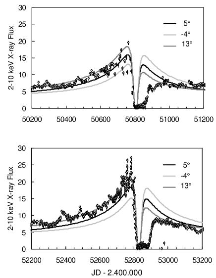
Figure 3: Details of the X-ray emission model without precession and nutation, close to the epochs of the two shallow minima, for three different values for the precession phase $\theta_{0p}$: $-4^{\circ},5^{\circ}$ and $13^{\circ}$. All other model parameters are shown in Table 1.

Figure 4: Variations with orbital phase of the wind velocity, mass loss rate, wind density at the contact surface, and latitude at the intersection of $\eta$ Carinae with the orbital plane facing the companion star. The first two quantities, given by the left axis, are relative to their values at $\lambda=90^{\circ}$, the latitude values, in degrees, are given in the right axis. The wind density, relative to its value at $\lambda=90^{\circ}$, in units of $1.5\times 10^{11}$ cm^-1 is also displayed at the right axis.

3 Results

We used equations (1) to (12) to model the X-ray light curve of $\eta$ Carinae, with the orbital parameters listed in the first column of Table 1. No formal fitting was attempted; instead, the model parameters were changed until they reproduced the general shape of the light curve (except the shallow minima), and the amplitude and period of the oscillations that occurred just before them. The parameters that fulfilled these criteria are listed in the last column of Table 1, and the model superposed to the observed light curve is presented in Figure 2; the two upper graphs represent the model without nodding motions ($\Delta\varphi=0$), and the last two graphs include nodding. The multiplicative term $G(t)$ in equation (5) was fitted by a function $G(t)=G_{0}[1+C_{x}(t-t_{0})]$, with $G_{0}$ and $C_{x}$ having constant values. The quoted errors were obtained by changing the values of each parameter while keeping the others constant until the model was no longer acceptable. As mentioned before, no formal fitting was attempted, but the combination of model parameters could not be changed arbitrarily, since each of them affect some particular feature of the X-ray light curve, as discussed bellow.

The parameters $\Omega$ and $\theta_{0p}$ are responsible for the asymmetry in the light curve at both sides of the shallow minima, as can be seen in the first two graphs in Figure 2. To illustrate this dependence, we plotted in Figure 3 the model light curves close to the minima for $\Omega=0.975$ and several values of $\theta_{0p}$, when no precession or nutation are present. We found that $\theta_{0p}=5\aas@@fstack{\circ}3$ reproduces well the asymmetry in the mean value of the light curve close to the minimum of 1997.9, but $\theta_{0p}\sim 13^{\circ}$ was necessary to reproduce the minimum of 2003.5. The difference in angles was attributed to the motion of the apsis, resulting in the precession period listed in Table 1. A large value of $\Omega$ was necessary to get the observed discontinuity; it indicates that $\eta$ Carinae is rotating at almost its critical velocity, as expected from the episodes of large mass loss. Of course, if other causes were responsible for the asymmetry in the X-ray light curve, like changes in opacity or stellar wind parameters, the value of these parameters should be revised.

The nutation parameters $P_{n}$, $\theta_{0n}$ and $\Delta\varphi$ are responsible for the amplitude and period of the large oscillations that occur before the minima, as can be seen in the two lower graphs in Figure 2; it is important to notice that, near periastron, the oscillations remained in phase in the two cycles for the same initial phase $\theta_{0n}$. However, the model does not reproduce the amplitude and the period of the oscillations far from periastron, which could be expected from the variation of the torque of the secondary star acting on $\eta$ Carinae.

The opacity parameter $C_{\tau}$ determines the shape of the light curve before the minima, and has no influence at other phases. The linear dependence of $G(t)$ with time implies an increase of about 30% in the X-ray intensity between the two cycles, which coincides with an increase in the optical flux during the same time interval (Martin et al., 2004) and could maybe attributed to an overall decrease in opacity.

No assumptions were made on the values of the mass loss rates and wind velocities of the binary stars. Instead, the value obtained for the model parameter $G_{0}$ and the comparison between the model hydrogen column density $N_{H}$ and that inferred from the XMM X-ray spectra observed far from periastron passage (Hamaguchi et al., 2007) allowed us to put some constrains on their magnitudes. From eq. (5) and assuming $\tau_{0}=0$ we can write:

$$\frac{\dot{M}_{s}^{2}}{V_{s}}=\frac{G_{0}}{1.83\times 10^{-10}}\eta^{1/2}(90^{\circ})$$ (19)

where

$$\eta(90^{\circ})=\frac{\dot{M}_{s}V_{s}}{\dot{M}_{p}(90^{\circ})V_{p}(90^{\circ})}=\frac{\dot{M}_{p}(\lambda)V_{p}(\lambda)}{\dot{M}_{p}(90^{\circ})V_{p}(90^{\circ})}\eta(\lambda)$$ (20)

From our model $\eta(90^{\circ})=0.15\,\eta(30^{\circ})$, resulting that for $\eta(30^{\circ})=0.2$ and $V_{s}=3000$ km s^-1, $\dot{M}_{s}=8\times 10^{-6}$ M_⊙ y^-1, well within the values of the mass loss rate of the secondary star used in the literature.

The hydrogen column density inferred from the X-ray spectra in January 2003 was $N_{H}=9\times 10^{22}$ cm^-2 (Hamaguchi et al., 2007). Using this value in equation (10) we obtain $\dot{M}_{p}/V_{p}=4.4\times 10^{14}$ g cm^-1, where we have used:

$$\int^{\infty}_{s_{\rm sh}}\frac{ds}{s^{2}+r_{0}^{2}}={\frac{1}{b\sin\Psi}}\biggl{(}\frac{\pi}{2}-\arctan{\frac{1}{\tan\Psi}}\biggr{)}=0.062\,\,{\rm AU}^{-1}$$ (21)

Assuming a wind velocity of 500 km s^-1 for $\eta$ Carinae, we find $\dot{M}_{p}=3.3\times 10^{-4}$ M_⊙ y^-1, also consistent with the values found in the literature.

Finally, the model opacity for January 2003 was $\tau_{p}=0.69$, which together with the observed hydrogen column density gives a value for $\sigma_{ph}=\tau_{p}/N_{H}=4.9$ cm² g^-1, consistent with the opacity to 3 keV photons of a 10⁴-10⁶ K gas (Parkin & Pittard, 2008).

From the inclination of the rotation axis of $\eta$ Carinae we estimated that, relative to the observer, the orbit has an inclination $i\sim 45^{\circ}-60^{\circ}$ , for $\eta$ varying between 0.2 and 0.1, as can be seen in Table 2. The variation of the wind velocity, mass loss rate and wind density along the orbital period, as well as the variation in $\lambda$ are shown in Figure 4 for the first orbital period.

Figure 5: Asymmetry parameter $k$ of the internal mass distribution of $\eta$ Carinae , produced by rotation and gravitational torque induced by the companion star, versus the ratio between the primary star radius and the orbital semi-major axis, for three values of the primary to secondary mass ratio $M_{s}/M_{p}$. Horizontal lines are the expected values of $k$ for polytropes of index $n=0$, 1, 2 and 3.

Although the eccentricity and period of the binary orbit used in the model agree with those used by other authors (Pittard et al., 1998; Ishibashi et al., 1999; Corcoran et al., 2001; Pittard & Corcoran, 2002; Okazaki et al., 2008), the value of $\theta_{0}$ is still controversial. The model presented in this paper was calculated for $\theta_{0}=-45^{\circ}$; changing its value to $\theta_{0}=+45^{\circ}$ will not have any effect on the X-ray emission but affect the absorption, mostly close to periastrom passage, where the model does not anyway reproduce the X-ray light curve; however, using $\theta_{0}=+45^{\circ}$ will not reproduce the shape and central velocity of the HeII$\lambda 4686$ and Paschen lines (Abraham & Falceta-Gonçalves, 2007; Falceta-Gonçalves & Abraham, 2009).

4 Discussion

As mentioned before, the model does not adjust the amplitude and period of the oscillations in the X-ray light curve far from periastrom passage. From Figure 2 we can also see that it does not reproduce the duration of the shallow minima. In fact, neither the analytical models nor the numerical simulations developed up to the present time were able to account for the extended minima as a result of X-ray photoelectric absorption by the dense wind of $\eta$ Carinae intercepting the line of sight (Pittard et al., 1998; Ishibashi et al., 1999; Corcoran et al., 2001; Pittard & Corcoran, 2002; Hamaguchi et al., 2007). Possible explanation are the increase in the H column density to $\sim 10^{24-26}$ cm^-2 due to additional material provided either by a slowly expanding shell of shocked material formed during periastron passage (Falceta-Gonçalves, Jatenco-Pereira & Abraham, 2005), or by the primary wind itself, which ”engulfs” the secondary star (Okazaki et al., 2008), or simply by the suppression of the secondary wind due to accretion of matter from the close primary star (Soker, 2005; Akashi, Socker & Behar, 2006) .

Figure 6: Angle $\Delta\varphi$ between the total and orbital angular momenta as a function of $R_{p}/A$ for several values of the mass ratio $M_{s}/M_{p}$. The horizontal line shows the value of $\Delta\varphi$ obtained from the model.

Figure 7: Time-scales for tidal friction $t_{TF}$, alignment $t_{alig}$, circularization $t_{circ}$, and synchronization $t_{spin}$ for $(M_{s}/M_{p}=0.4)$. The vertical line separates the regions where the orbit is unstable (left) and stable (right).

4.1 The orbital stability

The precession and nutation parameters are related to the torques of the secondary acting on the fast rotating non-spherical primary star and can provide constrains on the stellar masses, internal structure and orbital stability. Hut (1982) derived expressions for the evolution of the orbital and spin parameters in highly eccentric binary system, assuming that the tidal bulges lag by a constant angle from the line that joins the stars. Eggleton et al. (1998) obtained an expression for this angle, considering that the dissipative force is proportional to the rate of change of the quadrupole tensor of the stars, as seen by an observer that rotates with them.

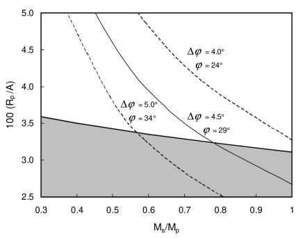
Figure 8: Relation between the mass ratio $M_{s}/M_{p}$ and $R_{p}/A$, for the combination of model parameters $(\varphi,\Delta\varphi)=(34^{\circ},5\aas@@fstack{\circ}0)$, $(29^{\circ},4\aas@@fstack{\circ}5)$, and $(24^{\circ},4\aas@@fstack{\circ}0)$. The shadowed region represents the parameter space in which the orbit is unstable.

The precession rate of the apsis, is independent of dissipation and, neglecting the torques of $\eta$ Carinae on the secondary star, can be expressed as:

$$\frac{P}{P_{p}} = 15\,kf(e)\biggl{(}\frac{M_{s}}{M_{p}}\biggr{)}\biggl{(}\frac{R_{p}}{A}\biggr{)}^{5}$$ (22)

$$+k\,\Omega^{2}g(e)\frac{(3\cos^{2}\varphi-1)}{4}\biggl{(}\frac{R_{p}}{A}\biggr{)}^{2}$$

with

$$f(e) = (1-e^{2})^{-5}(1+\frac{3}{2}e^{2}+\frac{1}{8}e^{4})$$ (23)

$$g(e) = (1-e^{2})^{-2},$$ (24)

where $k$ is the constant part of the quadrupole moment, which depends on the internal mass distribution of the primary star, $A$ is the semi-major axis of the orbit, and $R_{p}$ is the radius of the primary star.

In massive binary systems, the measured precession period $P_{p}$, together with the orbital parameters, stellar masses and radii, are used to calculate $k$ and improve the stellar structure models (e.g. Claret & Giménez, 1993). Since for $\eta$ Carinae the orbital and stellar parameters are unknown, we will take $M_{s}/M_{p}$ and $R_{p}/A$ as free parameters.

In Figure 5 we show the values of $k$ that satisfy equation (13) for $P/P_{p}=0.02$ (obtained from our model) as a function of $R_{p}/A$, for several values of $M_{s}/M_{p}$. The maximum value allowed for $R_{p}/A$ corresponds to the separation between the stars at periastron: $R_{p}/A=(1-e)=0.05$. The horizontal lines represent the values of $k$ for rotating polytropes with indices $n=0,1,2$ and 3 (Chandrasekhar, 1933); $n=0$ corresponds to a star with constant density while for $n=1$ the radius is independent of the central density.

Another constrain for the ratios $M_{s}/M_{p}$ and $R_{p}/A$ can be obtained from the amplitude of nutation $\Delta\varphi$, which represents the angle between the orbital and total angular momenta, and can be expressed as:

$$\cot\Delta\varphi=\cot\varphi+\frac{h}{I\omega\sin\varphi},$$ (25)

where $h$ is the orbital angular momentum, $I=M_{p}r_{g}^{2}R_{p}^{2}$ the momentum of inertia of the primary star and $r_{g}^{2}$ a parameter that depends on its internal structure. We can also write $h/I\omega$ in terms of $M_{s}/M_{p}$ and $R_{p}/A$:

$$\frac{h}{I\omega}=\frac{(1+M_{s}/M_{p})^{1/2}}{M_{s}/M_{p}}\biggl{(}\frac{R_{p}}{A}\biggr{)}^{1/2}\frac{1}{r_{g}^{2}\Omega(1-e^{2})^{1/2}},$$ (26)

In Figure 6 we present the relation between $\Delta\varphi$ and $R_{p}/A$ for $\varphi=29^{\circ}$ (obtained from our model), and $M_{s}/M_{p}=0.1$, 0.4, and 1.0. In the calculation, we used an interpolated relation between $r_{g}^{2}$ and $k$ for rotating polytropes obtained from Motz (1952):

$$\log r_{g}^{2}=0.453\log k-0.307$$ (27)

The value of $\Delta\varphi=4.5$ derived by fitting our model to the X-ray data is also shown in the figure. We can see that $M_{s}/M_{p}\sim 0.4$ represents the minimum value of the mass ratio for which a solution can be found. However, this result depends of the actual value of $r_{g}^{2}$, and should be consider only in the context of a consistency test for the parameters derived from the X-ray light curve.

The last parameter derived from the observations is the nutation period, which according to Eggleton et al. (1998) depends on both the conservative torques and those produced by tidal dissipation and can be written as:

$$\frac{P}{P_{n}} = \frac{k}{2r_{g}^{2}}\frac{M_{s}}{M_{p}}\biggl{(}1+\frac{M_{s}}{M_{p}}\biggr{)}^{-1/2}\biggl{(}\frac{R_{p}}{A}\biggr{)}^{3/2}\frac{\cos\varphi}{(1-e^{2})^{3/2}}$$

$$+ \frac{3}{8r_{g}^{2}}\frac{M_{s}}{M_{p}}\biggl{(}1+\frac{M_{s}}{M_{p}}\biggr{)}^{-1}\biggl{(}\frac{A}{R_{p}}\biggr{)}^{2}\frac{e^{2}(1+1/6e^{2})}{(1-e^{2})^{9/2}}\frac{P}{2\pi t_{TF}},$$

where $t_{TF}$ is the tidal friction time scale.

When only non-dissipative torques, represented by the first tem in eq. (19), are considered, the nutation period turns out to be several orders of magnitude larger than that obtained from our model $(P_{n}\cong P/92)$ for any combination of $k$, $(R_{p}/A)$ and $(M_{s}/M_{p})$ given by equation (13); therefore, the observed nutation must be produced by the dissipative torques, i.e. the second term in eq. (19), and its value can be used to estimate the dissipative time-scale $t_{TF}$:

$$t_{TF}=\frac{3}{8r_{g}^{2}}\frac{M_{s}}{M_{p}}\biggl{(}1+\frac{M_{s}}{M_{p}}\biggr{)}^{-1}\biggl{(}\frac{A}{R_{p}}\biggr{)}^{2}\frac{e^{2}(1+1/6e^{2})}{(1-e^{2})^{9/2}}\frac{P_{n}}{2\pi}.$$ (29)

In Figure 7 we display $t_{TF}$ as a function of $R_{p}/A$ for $M_{s}/M_{p}=0.4$.

When the tidal dissipation time-scale is known, it is possible to determine the time-scales for spin alignment and synchronization, and orbit circularization, defined as:

$$\frac{y}{t_{y}}=\left|\frac{dy}{dt}\right|,$$ (30)

where $t_{y}=(t_{alig},t_{spin},t_{circ})$ for $y=(\varphi,\omega,e)$, respectively.

For the case of a highly eccentric orbit, they can be obtained from Hut (1982):

$$t_{alig}=t_{TF}\biggl{[}\frac{693}{16}\frac{k}{r_{g}^{2}}\biggl{(}\frac{M_{s}}{M_{p}}\biggr{)}^{2}\biggl{(}\frac{R_{p}}{A}\biggr{)}^{6}\frac{H_{1}}{(1-e^{2})^{6}}\biggr{]}^{-1},$$ (31)

$$t_{spin}=t_{TF}\biggl{[}\frac{693}{16}\frac{k}{r_{g}^{2}}\biggl{(}\frac{M_{s}}{M_{p}}\biggr{)}^{2}\biggl{(}\frac{R_{p}}{A}\biggr{)}^{6}\frac{H_{2}}{(1-e^{2})^{6}}\biggr{]}^{-1},$$ (32)

$$t_{circ}=t_{TF}\biggl{[}\frac{11583}{64}k\biggl{(}1+\frac{M_{s}}{M_{p}}\biggr{)}\biggl{(}\frac{R_{p}}{A}\biggr{)}^{8}\frac{H_{3}}{(1-e^{2})^{13/2}}\biggr{]}^{-1},$$ (33)

with

$$H_{1} = \frac{h_{1}(\varepsilon)}{\Omega}\biggl{(}1+\frac{M_{s}}{M_{p}}\biggr{)}^{1/2}\biggl{(}\frac{R_{p}}{A}\biggr{)}^{3/2}$$ (34)

$$- \frac{20}{33}\frac{(1-e^{2})^{3/2}}{(1+e)^{2}}(1-\eta)h_{2}(\epsilon),$$

$$H_{2} = \frac{h_{1}(\varepsilon)}{\Omega}\biggl{(}1+\frac{M_{s}}{M_{p}}\biggr{)}\biggl{(}\frac{R_{p}}{A}\biggr{)}^{3/2}$$ (35)

$$- \frac{40}{33}\frac{(1-e^{2})^{3/2}}{(1+e)^{2}}h_{2}(\epsilon),$$

$$H_{3} = h_{3}(\varepsilon)$$

$$- h_{4}(\varepsilon)\Omega\frac{112}{117}\frac{(1-e^{2})^{3/2}}{(1+e)^{2}}\biggl{(}1+\frac{M_{s}}{M_{p}}\biggr{)}^{-1/2}\biggl{(}\frac{R_{p}}{A}\biggr{)}^{-3/2}$$

$$\eta=\frac{I\omega}{h},$$ (37)

$$\epsilon=1-e$$ (38)

$$h_{1}(\varepsilon)=1-\frac{30}{11}\varepsilon+\frac{35}{11}\varepsilon^{2}-\frac{460}{231}\varepsilon^{3}+\frac{5}{7}\varepsilon^{4}-\frac{10}{77}\varepsilon^{5}\frac{5}{231}\varepsilon^{6},$$ (39)

$$h_{2}(\varepsilon)=1-\frac{19}{7}\varepsilon+\frac{443}{140}\varepsilon^{2}-\frac{69}{35}\varepsilon^{3}+\frac{51}{70}\varepsilon^{4}-\frac{6}{35}\varepsilon^{5}\frac{3}{140}\varepsilon^{6}.$$ (40)

$$h_{3}(\varepsilon)=1-\frac{30}{13}\varepsilon+\frac{345}{143}\varepsilon^{2}-\frac{580}{429}\varepsilon^{3}+\frac{5}{11}\varepsilon^{4}-\frac{10}{143}\varepsilon^{5}\frac{5}{429}\varepsilon^{6},$$ (41)

$$h_{4}(\varepsilon)=1-\frac{7}{3}\varepsilon+\frac{205}{84}\varepsilon^{2}-\frac{29}{21}\varepsilon^{3}+\frac{19}{42}\varepsilon^{4}-\frac{2}{21}\varepsilon^{5}\frac{1}{84}\varepsilon^{6}.$$ (42)

In Figure 7 we plotted $t_{alig},t_{spin}$, and $t_{circ}$ as a function of $R_{p}/A$ for $M_{s}/M_{p}=0.4$. We can see that although $T_{TF}$ is of the order of $10^{5}$ years, the timescales for alignment, synchronization and circularization are larger than $10^{9}$ years, which means that the binary system did not reached yet its equilibrium configuration, considering an evolution timescale of $10^{6}-10^{7}$ years for the massive stars.

We should notice in eq. (27) that $H_{3}$ can be negative, implying that the eccentricity can increase with time, which corresponds to an unstable orbit. This occurs when the spin of the primary star is larger than the orbital angular velocity at periastron, or:

$$\frac{R_{p}}{A}<\frac{1-e^{2}}{(1+e)^{3/2}}\frac{1}{(1+M_{s}/M_{p})^{1/3}}$$ (43)

For $M_{s}/M_{p}=0.4$ this occurs when $R_{p}/A=0.035$, this value is shown as a vertical line in fig. (7). The general relation given by eq. (34) is shown in Figure 8; the shadowed area represents the parameter space for which the orbit is unstable. In the same Figure we show the lines that satisfy eq. (16), for the parameters found in our model $(\varphi=29^{\circ},\Delta\varphi=4\aas@@fstack{\circ}5)$, and for their extremes given by the uncertainties $(\varphi=34^{\circ},\Delta\varphi=5\aas@@fstack{\circ}0)$ and $(\varphi=24^{\circ},\Delta\varphi=4\aas@@fstack{\circ}0)$. The values of $M_{s}/M_{p}$ and $R_{p}/A$ for the binary system should lie between these two extreme lines.

5 Conclusions

We were able to reproduce the general features of the 2-10 keV X-ray light curve of $\eta$ Carinae obtained by $RXTE$ (Corcoran, 2005) during two cycles, including the amplitudes and phases of the short period oscillations that occurred prior to the shallow minima, assuming that the star rotates around an axis that is not perpendicular to the orbital plane, so that the secondary star faces $\eta$ Carinae at different latitudes as it moves along the orbit, using the fact that both the mass loss rate and the terminal wind velocity of $\eta$ Carinae are latitude dependent. According to the model, the star should be rotating with a fraction $\Omega=0.975$ of its critical velocity around an axis that forms an angle of about $29^{\circ}$ with the axis of the orbital plane, nutates with an amplitude of about $5^{\circ}$ and a period of 22.5 days. We also found that the line of apsis precesses with a period of about 274 years. According to the results of Abraham & Falceta-Gonçalves (2007), the inclination obtained for the rotation axis of $\eta$ Carinae implies that the inclination of the binary orbit relative to the observer must be $i\sim 45^{\circ}-60^{\circ}$, depending on the ratio of the wind momenta ($\eta\sim 0.2-0.1$). To fit the overall amplitude of the X-ray light curve, we calculated the phase and latitude dependent opacity due to the wind of $\eta$ Carinae intercepting the line of sight, and introduced a phase independent absorption, which decreased linearly with time and explained the overall increase in the X-ray flux between the two cycles. We used the precession period and nutation amplitude and rate to constrain the mass ratio of the binary system and the radius of the primary star relative to the semi-major orbital axis. We found that the orbit is stable if the radius of $\eta$ Carinae is larger than 0.035 times the orbit major axis, and the mass of the companion star at least half the mass of $\eta$ Carinae. Finally we found that for stable orbits, the time scale for orbit circularization, spin alignment and synchronization is much larger than the lifetime of the stars.

References

- Abraham & Falceta-Gonçalves (2007) Abraham, Z. & Falceta-Gonçalves, D. 2007, MNRAS, 378, 309
- Abraham et al. (2005) Abraham, Z., Falceta-Gonçalves, D., Dominici, T. P., Caproni, A. & Jatenco-Pereira V. 2005, MNRAS, 364, 922
- Akashi, Socker & Behar (2006) Akashi, M., Soker, N., Behar, E., 2006, ApJ, 644, 451
- Chandrasekhar (1933) Chandrasekhar, S., 1933, MNRAS, 93, 456
- e.g. Claret & Giménez (1993) Claret, A., Giménez, A., 1993, A&A, 277, 487
- Corcoran et al. (2001) Corcoran, M. F., Ishibashi, K., Swank, J. H. & Petre, R. 2001, ApJ, 547, 1039
- Corcoran (2005) Corcoran, M. F. 2005, AJ, 129, 2018
- Davidson et al. (2001) Davidson, K., Smith, N., Gull, T.R., Ishibashi, K. & Hillier, D.J. 2001, AJ, 121, 1569
- Dwarkadas & Owocki (2002) Dwarkadas, V.V. & Owocki, S.P. 2002, ApJ, 581, 1337
- Eggleton, Kiseleva & Hut (1998) Eggleton, P. P., Kiseleva, L., Hut, P., 1998, ApJ, 499, 853
- Falceta-Gonçalves, Jatenco-Pereira & Abraham (2005) Falceta-Gonçalves, D., Jatenco-Pereira, V. & Abraham, Z. 2005, MNRAS, 357, 895
- Falceta-Gonçalves & Abraham (2009) Falceta-Gonçalves, D., Abraham, Z. 2009, MNRAS, in press
- Kashi & Soker (2007) Kashi, A, Soker, N., 2007,New Astron., 12, 590
- Hamaguchi et al. (2007) Hamaguchi, K., Corcoran, M. F., Gull, T., Ishibashi, K., Pittard, J. M., et al. 2007, ApJ, 663, 522
- Hut (1982) Hut, P., 1982, A&A, 110, 37
- Ishibashi et al. (1999) Ishibashi, K., Corcoran, M. F., Davidson, K., Swank, J. H., Petre, R. et al. 1999, ApJ, 524, 983
- Martin et al. (2004) Martin, J. C., Koppelman, M. D., and the Treasury Project Team, 2004, AJ, 127, 2352
- Martin, Davis & Koppelman (2006) Martin, J. C., Davis, K. & Koppelman, M. D. 2006, AJ, 132, 2717
- Motz (1952) Motz, L., 1952, ApJ, 115,562
- Okazaki et al. (2008) Okazaki, A.T., Owocki, S.P., Russell, C.M., Corcoran, M.F., 2008, MNRAS, 388, 39
- Parkin & Pittard (2008) Parkin, E. R., Pittard, J. M., 2008, MNRAS, 388, 1047
- Parkin et al. (2009) Parkin, E. R., Pittard, J. M., Corcoran, M. F.,Hamaguchi, K., Stevens, I. R., 2009, MNRAS, 394, 1758
- Pittard & Corcoran (2002) Pittard, J. M. & Corcoran, M. F. 2002, A&A, 383, 636
- Pittard et al. (1998) Pittard, J. M., Stevens, I. R., Corcoran, M. F. & Ishibashi, K. 1998, MNRAS, 299, L5
- Pittard & Stevens (2002) Pittard, J. M. & Stevens, I.R. 2002, A&A, 388, L20
- Smith (2002) Smith, N. 2002, MNRAS, 337, 1252
- Smith (2006) Smith, N. 2006, ApJ, 644, 1151
- Soker (2005) Soker, N., 2005, ApJ, 635, 540
- Stahl et al. (2005) Stahl O., Weis K., Bomans D. J. et al. 2005, A&A, 435, 303
- Steiner & Damineli (2004) Steiner J. E. & Damineli A. 2004, ApJ, 612, L36
- Usov (1992) Usov, V.V. 1992, ApJ, 389, 635