Exclusive decays of $\chi_{bJ}$ and $\eta_{b}$ into two charmed mesons

Abstract

We develop a framework to study the exclusive two-body decays of bottomonium into two charmed mesons and apply it to study the decays of the $C$-even bottomonia. Using a sequence of effective field theories, we take advantage of the separation between the scales contributing to the decay processes, $2m_{b}\gg m_{c}\gg\Lambda_{\text{QCD}}$. We prove that, at leading order in the EFT power counting, the decay rate factorizes into the convolution of two perturbative matching coefficients and three non-perturbative matrix elements, one for each hadron. We calculate the relations between the decay rate and non-perturbative bottomonium and $D$-meson matrix elements at leading order, with next-to-leading log resummation. The phenomenological implications of these relations are discussed.

I Introduction

The exclusive two-body decays of heavy quarkonium into light hadrons have been studied in the framework of perturbative QCD by many authors (for reviews, see Chernyak:1983ej Brodsky:1989pv ). These processes exhibit a large hierarchy between the heavy quark mass, which sets the scale for annihilation processes, and the scales that determine the dynamical structure of the particles in the initial and final states. The large energy released in the annihilation of the heavy quark-antiquark pair and the kinematics of the decay — with the products flying away from the decay point in two back-to-back, almost light-like directions— allow for rigorously deriving a factorization formula for the decay rate at leading twist (for an up-to-date review of the theoretical and experimental status of the exclusive decays into light hadrons, see Brambilla:2004wf ).

For the bottomonium system, a particularly interesting class of two-body final states is the ones containing two charmed mesons. In these cases the picture is complicated by the appearance of an additional intermediate scale, the charm mass $m_{c}$, which is much smaller than the bottom mass $m_{b}$ but is large enough to be perturbative. These decays differ significantly from those involving only light quarks. The creation of mesons that are made up of purely light quarks involves creating two quark-antiquark pairs, with the energy shared between the quark and antiquark in each pair. In the production of two $D$ mesons, however, almost all the energy of the bottomonium is carried away by the heavy $c$ and $\bar{c}$, while the light quark and antiquark, which bind to the $\bar{c}$ and $c$ respectively, carry away (boosted) residual energies.

The existence of well-separated scales in the system and the intuitive picture of the decay process suggest to tackle the problem using a sequence of effective field theories (EFTs) that are obtained by subsequently integrating out the dynamics relevant to the perturbative scales $m_{b}$ and $m_{c}$.

In the first step, we integrate out the scale $m_{b}$ by describing the $b$ and $\bar{b}$ with Non-Relativistic QCD (NRQCD) Bodwin:1994jh , and the highly energetic $c$ and $\bar{c}$ with two copies of Soft-Collinear Effective Theory (SCET) Bauer:2000ew Bauer:2000yr Bauer:2001yt Bauer:2002nz Leibovich:2003jd in opposite light-cone directions. In the second step, we integrate out the dynamics manifested at scales of order $m_{c}$ by treating the quarkonium with potential NRQCD (pNRQCD) Pineda:1997bj Brambilla:1999xf Brambilla:2004jw , and the $D$ mesons with a boosted version of Heavy-Quark Effective Theory (HQET) Grinstein:1990mj Eichten:1989zv Georgi:1990um Beneke:2003xh Beneke:2004km Fleming:2007qr Fleming:2007xt . The detailed explanation of why the aforementioned EFTs are employed is offered in Sec. II. We will prove that, at leading order in the EFT expansion, the decay rate factors into a convolution of two perturbative matching coefficients and three (one for each hadron) non-perturbative matrix elements. The non-perturbative matrix elements are process-independent and encode information on both the initial and final states.

For simplicity, in this paper we focus on the decays of the $C$-even quarkonia $\chi_{bJ}$ and $\eta_{b}$ that, at leading order in the strong coupling $\alpha_{s}$, proceed via the emission of two virtual gluons. The same method can be generalized to the decays of $C$-odd states $\Upsilon$ and $h_{b}$, which require an additional virtual gluon. We also refrain from processes that have vanishing contributions at leading order in the EFT power counting. So the specific processes studied in this paper are $\chi_{b0,2}\rightarrow DD$, $\chi_{b0,\,2}\rightarrow D^{*}D^{*}$, and $\eta_{b}\rightarrow DD^{*}+\text{c.c.}$ However, the EFT approach developed in this paper enables one to systematically include power-suppressed effects, making it possible to go beyond the leading-twist approximation.

The study of the inclusive and exclusive charm production in bottomonium decays and of the role played by the charm mass $m_{c}$ in such processes have recently drawn renewed attention Bodwin:2007zf Kang:2007uv Braguta:2009df Braguta:2009xu , in connection with the experimental advances spurred in the past few years by the abundance of bottomonium data produced at facilities like BABAR, BELLE, and CLEO. The most notable result was the observation of the bottomonium ground state $\eta_{b}$, recently reported by the BABAR collaboration :2008vj . Furthermore, the CLEO collaboration published the first results for several exclusive decays of $\chi_{b}$ into light hadrons :2008sx and for the inclusive decay of $\chi_{b}$ into open charm Briere:2008cv . In particular, they measured the branching ratio $\mathcal{B}(\chi_{bJ}\rightarrow D^{0}X)$, where $J$ is the total angular momentum of the $\chi_{b}$ state, and conclusively showed that for $J=1$ the production of open charm is substantial: $\mathcal{B}(\chi_{b1}(1P)\rightarrow D^{0}X)=12.59\pm 1.94\%$. For the $J=0,2$ states the data are weaker, but the production of open charm still appears to be relevant. The measurements of the CLEO collaboration are in good agreement with the prediction of Bodwin et al. Bodwin:2007zf , where EFT techniques (in particular NRQCD) were for the first time applied to study the production of charm in bottomonium decays.

The double-charm decay channels analyzed here have not yet been observed, so one of our aims is to see if they may be observable given the current data. Unfortunately, the poor knowledge of the $D$-meson matrix elements prevents us from providing definitive predictions for the decay rates $\Gamma(\chi_{bJ}\rightarrow DD)$, $\Gamma(\chi_{bJ}\rightarrow D^{*}D^{*})$, and $\Gamma(\eta_{b}\rightarrow DD^{*}+\textrm{c.c.})$. As we will show, these rates are indeed strongly dependent on the parameters of the $D$- and $D^{*}$-meson distribution amplitudes, in particular on their first inverse moments $\lambda_{D}$ and $\lambda_{D^{*}}$: the rates vary by an order of magnitude in the accepted ranges for $\lambda_{D}$ and $\lambda_{D^{*}}$. On the other hand, the factorization formula implies that these channels, if measured with sufficient accuracy, could constrain the form of the $D$-meson distribution amplitude and the value of its first inverse moment. In turn, the details of the $D$-meson structure are relevant to other $D$-meson observables, which are crucial for a model-independent determination of the CKM matrix elements $|V_{cd}|$ and $|V_{cs}|$ Hill:2005ju .

This paper is organized as follows. In Sec. II we discuss the degrees of freedom and the EFTs we use. In Sec. III.1 we match QCD onto NRQCD and SCET at the scale $2m_{b}$. The renormalization-group equation (RGE) for the matching coefficient is derived and solved in Sec. III.2. In Sec. IV.1 the scale $m_{c}$ is integrated out by matching NRQCD and SCET onto pNRQCD and bHQET. The renormalization of the low-energy EFT operators is performed in Sec. IV.2, with some technical details left to App. A. The decay rates are calculated in Sec. V using two model distribution amplitudes. In Sec. VI we draw our conclusions.

II Degrees of freedom and the Effective Field Theories

Several well-separated scales are involved in the decays of the $C$-even bottomonia $\eta_{b}$ and $\chi_{bJ}$ into two $D$ mesons, making them ideal processes for the application of EFT techniques. The distinctive structures of the bottomonium (a heavy quark-antiquark pair) and the $D$ meson (a bound state of a heavy quark and a light quark) suggest that one needs different EFTs to describe the initial and final states.

We first look at the initial state. The $\eta_{b}$ is the ground state of the bottomonium system. It is a pseudoscalar particle, with spin $S=0$, orbital angular momentum $L=0$, and total angular momentum $J=0$. In what follows we will often use the spectroscopic notation ${}^{2S+1}L_{J}$, in which the $\eta_{b}$ is denoted by ${}^{1}S_{0}$. The $\chi_{bJ}$ is a triplet of states with quantum numbers ${}^{3}P_{J}$. The $\eta_{b}$ and $\chi_{bJ}$ are non-relativistic bound states of a $b$ quark and a $\bar{b}$ antiquark. The scales in the system are the $b$ quark mass $m_{b}$, the relative momentum of the $b\,\bar{b}$ pair $m_{b}w$, the binding energy $m_{b}w^{2}$, and $\Lambda_{\text{QCD}}$, the scale where QCD becomes strongly coupled. $w$ is the relative velocity of the quark-antiquark pair in the meson, and from the bottomonium spectrum it can be inferred that $w^{2}\sim 0.1$. Since $m_{b}\gg\Lambda_{\text{QCD}}$, $m_{b}$ can be integrated out in perturbation theory and the bottomonium can be described in NRQCD. The degrees of freedom of NRQCD are non-relativistic heavy quarks and antiquarks, with energy and momentum $(E,|\vec{p}\,|)$ of order $(m_{b}w^{2},m_{b}w)$, light quarks and gluons. In NRQCD, the gluons can be soft $(m_{b}w,m_{b}w)$, potential $(m_{b}w^{2},m_{b}w)$, and ultrasoft (usoft) $(m_{b}w^{2},m_{b}w^{2})$. The NRQCD Lagrangian is constructed as a systematic expansion in $1/m_{b}$ whose first few terms are

$$\mathcal{L}_{\rm{NRQCD}}=\psi^{\dagger}\left(iD_{0}+\frac{\vec{D}^{2}}{2m_{b}}+\frac{\vec{\sigma}\cdot g\vec{B}}{2m_{b}}+\ldots\right)\psi+\chi^{\dagger}\left(iD_{0}-\frac{\vec{D}^{2}}{2m_{b}}-\frac{\vec{\sigma}\cdot g\vec{B}}{2m_{b}}+\ldots\right)\chi\;,$$

where $\psi$ and $\chi^{\dagger}$ annihilate a $b$ quark and a $\bar{b}$ antiquark respectively, and $\cdots$ denotes higher-order contributions in $1/m_{b}$. In NRQCD several mass scales are still dynamical and different assumptions on the hierarchy of these scales may lead to different power countings for operators of higher dimensionality. However, as long as $w\ll 1$, higher-dimension operators are suppressed by powers of $w$ (for a critical discussion on the different power countings we refer to Brambilla:2004jw ).

NRQCD still contains interactions that can excite the heavy quarkonium far from its mass shell, for example, through the interaction of a non-relativistic quark with a soft gluon. In the case $m_{b}w\gg\Lambda_{\text{QCD}}$, we can integrate out these fluctuations, matching perturbatively NRQCD onto a low-energy effective theory, pNRQCD. We are then left with a theory of non-relativistic quarks and ultrasoft gluons, with non-local potentials induced by the integration over soft- and potential-gluon modes. The interactions of the heavy quark with ultrasoft gluons are still described by the NRQCD Lagrangian, with the constraint that all the gluons are ultrasoft. In the weak coupling regime $m_{b}w\gg\Lambda_{\text{QCD}}$, the potentials are organized by an expansion in $\alpha_{s}(m_{b}w)$, $1/m_{b}$, and $r$, where $r$ is the distance between the quark and antiquark in the quarkonium, $r\sim 1/m_{b}w$. If we assume $m_{b}w^{2}\sim\Lambda_{\text{QCD}}$, each term in the expansion has a definite power counting in $w$ and the leading potential is Coulombic $V\sim\alpha_{s}(m_{b}w)/r$.

An alternative approach, which does not require a two-step matching, has been developed in the effective theory vNRQCD Luke:1996hj Luke:1999kz Manohar:1999xd Hoang:2002yy . In the vNRQCD approach there is only one EFT below $m_{b}$, which is obtained by integrating out all the off-shell fluctuations at the hard scale $m_{b}$ and introducing different fields for various propagating degrees of freedom (non-relativistic quarks and soft and ultrasoft gluons). In spite of the differences between the two formalisms, pNRQCD and vNRQCD give equivalent final answers in all the known examples in which both theories can be applied.

We now turn to the structure of the $D$ meson. The most relevant features of the $D$ meson are captured by a description in HQET. In HQET, in order to integrate out the inert scale $m_{c}$, the momentum of the heavy quark is generically written as Georgi:1990um

$$p=m_{c}v+k\;,$$ (1)

where $v$ is the four-velocity label, satisfying $v^{2}=1$, and $k$ is the residual momentum. If one chooses $v$ to be the center-of-mass velocity of the $D$ meson, $k$ scales as $k\sim v\Lambda_{\text{QCD}}$. Introducing the light-cone vectors $n^{\mu}=(1,0,0,1)$ and $\bar{n}^{\mu}=(1,0,0,-1)$, one can express the residual momentum in light-cone coordinates, $k^{\mu}=\bar{n}\cdot k\,n^{\mu}/2+n\cdot k\,\bar{n}^{\mu}/2+k^{\mu}_{\perp}$ or simply $k=(n\cdot k,\bar{n}\cdot k,\vec{k}_{\perp})$. There are two relevant frames. One is the $D$-meson rest frame, in which $v$ is conveniently chosen as $v_{0}=(1,0,0,0)$, and the other is the bottomonium rest frame, in which the $D$ mesons are highly boosted in opposite directions, with $v$ chosen as $v=v_{D}$, the four-velocity of one of the $D$ mesons. By a simple consideration of kinematics and the scaling $k\sim v\Lambda_{\text{QCD}}$, one can work out the scalings for $k$ in the two frames. In the $D$-meson rest frame, $k\sim\Lambda_{\text{QCD}}(1,1,1)$, and in the bottomonium rest frame (supposing the $D$ meson moving in the positive $z$-direction),

$$k\sim\Lambda_{\text{QCD}}\left(n\cdot v_{D},\bar{n}\cdot v_{D},1\right)\sim\Lambda_{\text{QCD}}\bar{n}\cdot v_{D}\left(\lambda^{2},1,\lambda\right)\;,$$ (2)

where $\bar{n}\cdot v_{D}\sim 2m_{b}/m_{c}$ and $\lambda=m_{c}/2m_{b}\ll 1$. It is convenient for the calculation in this paper to use the bottomonium rest frame, so we drop the subscript in $v_{D}$ and we assume $v=v_{D}$ in the rest of this paper. The momentum scaling in Eq. (2) is called ultracollinear (ucollinear), and boosted HQET (bHQET) is the theory that describes heavy quarks with ultracollinear residual momenta and light degrees of freedom (including gluons and light quarks) with the same momentum scaling.

The bHQET Lagrangian is organized as a series in powers of $\Lambda_{\text{QCD}}/m_{c}$ and, for residual momentum ultracollinear in the $n$-direction, the leading term is Fleming:2007qr

$$\mathcal{L}_{\rm{bHQET}}=\bar{h}_{n}iv\cdot Dh_{n}\;,$$ (3)

where the field $h_{n}$ annihilates a heavy quark and the covariant derivative $D$ contains ultracollinear and ultrasoft gluons,

$$iD^{\mu}=\frac{n^{\mu}}{2}\left(i\bar{n}\cdot\partial+g\bar{n}\cdot A_{n}\right)+\frac{\bar{n}^{\mu}}{2}\left(in\cdot\partial+gn\cdot A_{n}+gn\cdot A_{us}\right)+\left(i\partial^{\mu}_{\perp}+gA^{\mu}_{n,\,\perp}\right)\;.$$ (4)

The ultrasoft gluons only enter in the small component of the covariant derivative. This fact can be exploited to decouple ultrasoft and ultracollinear modes in the leading-order Lagrangian through a field redefinition reminiscent of the collinear-ultrasoft decoupling in SCET Bauer:2001yt Fleming:2007qr . The ultracollinear-ultrasoft decoupling is an essential ingredient for the factorization of the decay rate.

Therefore, the appropriate EFT to calculate the decay rate is a combination of pNRQCD, for the bottomonium, and two copies of bHQET, with fields collinear to the $n$ and $\bar{n}$ directions, for the $D$ and $\bar{D}$ mesons, symbolically written as $\text{EFT}_{\text{II}}\equiv\text{pNRQCD}+\text{bHQET}$.

As we mentioned earlier, we plan to describe the bottomonium structure with a two-step scheme $\text{QCD}\to\text{NRQCD}\to\text{pNRQCD}$. However, at the intermediate stage, where we first integrate out the hard scale $2m_{b}$ and arrive at the scale $m_{b}w$, the $D$ meson cannot yet be described in bHQET. This is because the interactions relevant at the intermediate scale $m_{b}w$ can change the $c$-quark velocity and leave the $D$ meson off-shell of order $\sim(m_{b}w)^{2}\sim m^{2}_{c}\gg\Lambda_{\text{QCD}}^{2}$. Highly energetic $c$ and $\bar{c}$ travelling in opposite directions can be described properly by SCET with mass. Thus, at the scale $\mu=2m_{b}$, we match QCD onto an intermediate EFT, $\text{EFT}_{\text{I}}\equiv\text{NRQCD}+\text{SCET}$, in which the EFT expansion is organized by $\lambda$ and $w$. The degrees of freedom of $\text{EFT}_{\text{I}}$ are tabulated in Tab. 1.

	NRQCD	field	momentum	SCET	field	momentum
quark	$b$, $\bar{b}$	$\psi_{b}$,  $\chi_{\bar{b}}$	$(m_{b}w^{2},m_{b}w)$	$c$, $\bar{c}$	$\xi^{c}_{\bar{n}}$,   $\xi^{\bar{c}}_{n}$	$2m_{b}(1,\lambda^{2},\lambda)$,   $2m_{b}(\lambda^{2},1,\lambda)$
gluon	potential	$A^{\mu}$	$(m_{b}w^{2},m_{b}w)$	collinear	$A^{\mu}_{\bar{n}}$,   $A^{\mu}_{n}$	$2m_{b}(1,\lambda^{2},\lambda)$,   $2m_{b}(\lambda^{2},1,\lambda)$
	soft	$A^{\mu}$	$(m_{b}w,m_{b}w)$	soft	$A^{\mu}_{s}$	$2m_{b}(\lambda,\lambda,\lambda)$
	usoft	$A^{\mu}$	$(m_{b}w^{2},m_{b}w^{2})$	usoft	$A^{\mu}_{us}$	$2m_{b}(\lambda^{2},\lambda^{2},\lambda^{2})$

Table 1: Degrees of freedom in $\text{EFT}_{\text{I}}(\text{NRQCD}+\text{SCET})$. $w$ is the $b\,\bar{b}$ relative velocity in the bottomonium rest frame, while $\lambda\sim m_{c}/2m_{b}$ is the SCET expansion parameter. We assume $m_{b}w\sim m_{c}$ (or, equivalently, $w\sim\lambda$) and $m_{b}w^{2}\sim m_{b}\lambda^{2}\sim\Lambda_{\text{QCD}}$.

Then, we integrate out $m_{c}$ and $m_{b}w$ at the same time, matching $\text{EFT}_{\text{I}}$ onto $\text{EFT}_{\text{II}}$ at the scale $\mu^{\prime}=m_{c}$. In $\text{EFT}_{\text{II}}$, the low-energy approximation is organized by $\Lambda_{\text{QCD}}/m_{c}$ and $w$. The degrees of freedom of $\text{EFT}_{\text{II}}$ are summarized in Tab. 2. When no subscript is specified in the rest of this paper, any reference to EFT applies to both $\text{EFT}_{\text{I}}$ and $\text{EFT}_{\text{II}}$. To facilitate the power counting, we adopt $w\sim\lambda\sim\Lambda_{\text{QCD}}/m_{c}$. As a first study, we will perform in this paper the leading-order calculation of the bottomonium decay rates.

	pNRQCD	field	momentum	bHQET	field	momentum
quark	$b$, $\bar{b}$	$\psi_{b}$,  $\chi_{\bar{b}}$	$(m_{b}w^{2},m_{b}w)$	$c$, $\bar{c}$	$h^{c}_{\bar{n}}$,   $h^{\bar{c}}_{n}$	$Q\,(1,\lambda^{2},\lambda)$,   $Q\,(\lambda^{2},1,\lambda)$
				$u$, $d$	$\xi_{\bar{n}}$,   $\xi_{n}$	$Q\,(1,\lambda^{2},\lambda)$,   $Q\,(\lambda^{2},1,\lambda)$
gluon	usoft	$A^{\mu}$	$(m_{b}w^{2},m_{b}w^{2})$	usoft	$A^{\mu}_{us}$	$Q(\lambda,\lambda,\lambda)$
				ucollinear	$A^{\mu}_{\bar{n}}$,   $A^{\mu}_{n}$	$Q\,(1,\lambda^{2},\lambda)$,   $Q\,(\lambda^{2},1,\lambda)$

Table 2: Degrees of freedom in $\text{EFT}_{\text{II}}(\text{pNRQCD}+\text{bHQET})$. The scale $Q$ in bHQET is $Q=n\cdot v^{\prime}\Lambda_{\text{QCD}}$ for the $\bar{n}$-collinear sector and $Q=\bar{n}\cdot v\Lambda_{\text{QCD}}$ for the $n$-collinear sector. $n\cdot v^{\prime}$ and $\bar{n}\cdot v$ are the large light-cone components of the $D$-meson velocities in the bottomonium rest frame, $n\cdot v^{\prime}\sim\bar{n}\cdot v\sim 2m_{b}/m_{c}$. $\lambda$ and $w$ are defined as in Tab. 1.

III $\text{NRQCD}+\text{SCET}$

III.1 Matching

In the first step, we integrate out the dynamics related to the hard scale $2m_{b}$ by matching the QCD diagrams for the production of a $c\,\bar{c}$ pair in the annihilation of a $b\,\bar{b}$ pair onto their $\text{EFT}_{\text{I}}$ counterparts. The tree-level diagrams for the process are shown in Fig. 1. The gluon propagator in the QCD diagram has off-shellness of order $q^{2}=(2m_{b})^{2}$ and it is not resolved in $\text{EFT}_{\text{I}}$, giving rise to a point-like interaction.

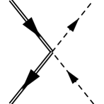
Figure 1: Matching QCD onto $\text{EFT}_{\text{I}}$. On the r.h.s., the double lines represent the non-relativistic $b$ ($\bar{b}$) (anti)quark, while the dashed lines represent the collinear $c$ ($\bar{c}$) (anti)quark.

We calculate the diagrams on shell, finding

$$iJ_{\rm{QCD}}=iC(\mu)J_{\text{EFT}_{\text{I}}}(\mu)\;,$$ (5)

with, at tree level,

$$J_{\text{EFT}_{\text{I}}}=\chi_{\bar{b}}^{\dagger}\sigma^{\mu}_{\perp}t^{a}\psi_{b}\;\bar{\chi}^{c}_{\bar{n}}\,S^{\dagger}_{\bar{n}}\,\gamma_{\mu\,\perp}t^{a}\,S_{n}\,\chi^{\bar{c}}_{n}\quad\text{and}\quad C(\mu=2m_{b})=\frac{\alpha_{s}(2m_{b})\pi}{m^{2}_{b}}\;,$$ (6)

where $t^{a}$ are color matrices and the symbol $\sigma^{\mu}$ denotes the four matrices $\sigma^{\mu}=(1,\vec{\sigma})$, with $\vec{\sigma}$ the Pauli matrices. The subscript $\perp$ refers to the components orthogonal to the light-cone vectors $n^{\mu}$ and $\bar{n}^{\mu}$. The fields $\psi_{b}$ and $\chi^{\dagger}_{\bar{b}}$ are two-component spinors that annihilate respectively a $b$ quark and a $\bar{b}$ antiquark. $\chi^{\bar{c}}_{n,\,\bar{n}\cdot p}$ and $\chi^{c}_{\bar{n},\,n\cdot p}$ are collinear gauge-invariant fermion fields:

$$\chi^{\bar{c}}_{n,\,\bar{n}\cdot p}\equiv(W_{n}^{\dagger}\xi^{\bar{c}}_{n})_{\bar{n}\cdot p}\;,\qquad\chi^{c}_{\bar{n},\,n\cdot p}\equiv(W_{\bar{n}}^{\dagger}\xi^{c}_{\bar{n}})_{n\cdot p}\;,$$ (7)

where $W_{n}$ is defined as

$$W_{n}\equiv\sum_{\rm{perms}}\exp\left(-\frac{g}{\bar{n}\cdot\mathcal{P}}\bar{n}\cdot A_{n}\right)\;.$$ (8)

$W_{\bar{n}}$ has an analogous definition with $n\rightarrow\bar{n}$. Collinear fields are labelled by the large component of their momentum. Note, however, we omit in Eq. (6) the subscripts $n\cdot p$ and $\bar{n}\cdot p$ of the collinear fermion fields, in order to simplify the notation. The operator $\bar{n}\cdot\mathcal{P}$ in the definition (8) is a label operator that extracts the large component of the momentum of a collinear field, $\bar{n}\cdot\mathcal{P}\,\phi_{n,\,\bar{n}\cdot p}=\bar{n}\cdot p\,\phi_{n,\,\bar{n}\cdot p}$, where $\phi_{n,\,\bar{n}\cdot p}$ is a generic collinear field. $S_{n(\bar{n})}$ is a soft Wilson line,

$$S_{n}\equiv\sum_{\rm{perms}}\left[\exp\left(-\frac{g}{n\cdot\mathcal{P}}n\cdot A_{s}\right)\right],$$ (9)

where the operator $n\cdot\mathcal{P}$ acts on soft fields, $n\cdot\mathcal{P}\,\phi_{s}=n\cdot k\,\phi_{s}$.

Since in SCET different gluon modes are represented by different fields, we have to guarantee the gauge invariance of the operator $J_{\text{EFT}_{\text{I}}}$ under separate soft and collinear gauge transformations. A soft transformation is defined by $V_{s}(x)=\exp{(i\beta^{a}_{s}t^{a})}$, with $\partial_{\mu}V\sim 2m_{b}(\lambda,\lambda,\lambda)$, while a gauge transformation $U(x)$ is $n$-collinear if $U(x)=\exp{(i\alpha^{a}(x)t^{a})}$ and $\partial_{\mu}U(x)\sim 2m_{b}(\lambda^{2},1,\lambda)$. It has been shown in Ref. Bauer:2001yt that collinear fields do not transform under a soft transformation and that the combination $W_{n}^{\dagger}\xi_{n}$ is gauge invariant under a collinear transformation. Soft fields do not transform under collinear transformations but they do under soft transformations. For example, the NRQCD quark and antiquark fields transform as $\psi_{b}\rightarrow V_{s}(x)\psi_{b}$. The soft Wilson line has the same transformation, $S_{n}\rightarrow V_{s}(x)S_{n}$. Therefore, $\chi_{\bar{b}}^{\dagger}\sigma^{\mu}_{\perp}t^{a}\psi_{b}$ transforms as an octet under soft gauge transformations. Since $\bar{\chi}^{c}_{\bar{n}}\,S^{\dagger}_{\bar{n}}\,\gamma_{\mu\,\perp}t^{a}\,S_{n}\,\chi^{\bar{c}}_{n}$ behaves like an octet as well, $J_{\text{EFT}_{\text{I}}}$ is invariant. It is worth noting that the soft Wilson lines are necessary to guarantee the gauge invariance of $J_{\text{EFT}_{\text{I}}}$. We have explicitly checked their appearance at one gluon by matching QCD diagrams like the one in Fig. 1, with all the possible attachments of an extra soft or collinear gluon, onto four-fermion operators in $\text{EFT}_{\text{I}}$.

III.2 Running

The matching coefficient $C$ and the effective operator $J_{\text{EFT}_{\text{I}}}$ depend on the renormalization scale $\mu$. Since the effective operator is sensitive to the low-energy scales in $\text{EFT}_{\text{I}}$, logarithms that would appear in the evaluation of $J_{\text{EFT}_{\text{I}}}$ are minimized by the choice $\mu\sim m_{c}$. On the other hand, since the coefficient encodes the high-energy dynamics of the scale $2m_{b}$, such a choice would induce large logarithms of $m_{c}/2m_{b}$ in the matching coefficient. These logarithms can be resummed using RGEs in $\text{NRQCD}+\text{SCET}$.

The $\mu$ dependence of $J_{\text{EFT}_{\text{I}}}$ is governed by an equation of the following form Manohar ,

$$\frac{d}{d\ln\mu}J_{\text{EFT}_{\text{I}}}(\mu)=-\gamma_{\text{EFT}_{\text{I}}}(\mu)J_{\text{EFT}_{\text{I}}}(\mu)\;,$$ (10)

where the anomalous dimension $\gamma_{\text{EFT}_{\text{I}}}$ is given by

$$\gamma_{\text{EFT}_{\text{I}}}=Z^{-1}_{\text{EFT}_{\text{I}}}\frac{d}{d\ln\mu}Z_{\text{EFT}_{\text{I}}}$$ (11)

and $Z_{\text{EFT}_{\text{I}}}$ is the counterterm that relates the bare operator $J^{(0)}_{\text{EFT}_{\text{I}}}$ to the renormalized one, $J^{(0)}_{\text{EFT}_{\text{I}}}=Z_{\text{EFT}_{\text{I}}}(\mu)J_{\text{EFT}_{\text{I}}}(\mu)$. Since the l.h.s. of Eq. (5) is independent of the scale $\mu$, the RGE (10) can be recast as an equation for the matching coefficient $C(\mu)$,

$$\begin{split}&\frac{d}{d\ln\mu}C(\mu)=\gamma_{\text{EFT}_{\text{I}}}(\mu)C(\mu)\;.\end{split}$$ (12)

The counterterm $Z_{\text{EFT}_{\text{I}}}$ cancels the divergences that appear in Green functions with the insertion of the operator $J_{\text{EFT}_{\text{I}}}$. We calculate $Z_{\text{EFT}_{\text{I}}}$ in the $\overline{\rm{MS}}$ scheme by evaluating the divergent part of the four-point Green function at one loop, given by the diagrams in Figs. 2 - 4.

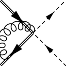
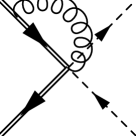
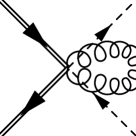
Figure 2: Soft diagrams at one loop.

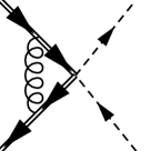
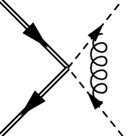
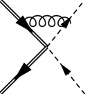
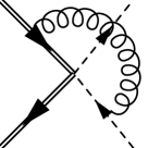
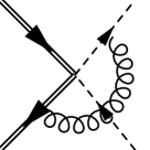
Figure 3: Ultrasoft diagrams at one loop.

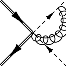
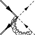
Figure 4: Collinear diagrams at one loop.

Since in NRQCD we do not introduce different gluon fields for different momentum modes, “soft” and “ultrasoft” in Fig. 2 and Fig. 3 refer to the convention that we impose soft or ultrasoft scaling to the corresponding loop momentum. The potential region, which should be considered in the diagrams of Fig. 2, does not give any divergent contribution.

The integrals are evaluated in dimensional regularization, with $d=4-2\varepsilon$. We regulate the infrared divergences by keeping the non-relativistic $b$ and $\bar{b}$ and the collinear $c$ and $\bar{c}$ off-shell: $E_{b,\,\bar{b}}-\vec{p}^{\;2}_{b,\,\bar{b}}/2m_{b}=\Delta_{b}$, $p^{2}_{c}-m^{2}_{c}=\Delta^{2}$ and $p^{2}_{\bar{c}}-m^{2}_{c}=\bar{\Delta}^{2}$. We power count the $c$-quark off-shellness as $\Delta^{2}\sim\bar{\Delta}^{2}\sim m_{b}^{2}\lambda^{2}$ and the $b$-quark off-shellness as $\Delta_{b}\sim m_{b}w^{2}$. We also assume $\Delta^{2},\,\bar{\Delta}^{2}>0$. To avoid double counting, we define the one-loop integrals with the $0$-bin subtraction Manohar:2006nz .

Even with an off-shellness, the soft diagrams in Fig. 2 do not contain any scale and they are completely cancelled by their 0-bin.

The divergent part of the ultrasoft diagrams in Fig. 3 is

$$\begin{split}i\mathcal{M}_{usoft}&=-i\frac{\alpha_{s}}{4\pi}\,\left\{2C_{F}\,\left[\frac{1}{\varepsilon^{2}}-\frac{1}{\varepsilon}\ln\left(\frac{\Delta^{2}\,\bar{\Delta}^{2}}{n\cdot p_{c}\bar{n}\cdot p_{\bar{c}}\,\mu^{2}}\right)\right]+\frac{1}{N_{c}}\frac{1}{\varepsilon}\ln(-1-i0)-\frac{1}{N_{c}}\,\frac{1}{\varepsilon}\right\}J_{\text{EFT}_{\text{I}}}\;,\end{split}$$ (13)

where $C_{F}=(N^{2}_{c}-1)/2N_{c}$ and $\mu$ is the $\overline{\rm{MS}}$ unit mass, $\mu^{2}=4\pi\mu^{2}_{\rm{MS}}\exp{(-\gamma_{E})}$. The first term in the curly brackets of Eq. (13) corresponds to the sum of the divergences in the second diagram in Fig. 3, where an ultrasoft gluon is exchanged between the $c$ and $\bar{c}$ quarks collinear in back-to-back directions, and those in the last four diagrams of the same figure, which contain ultrasoft interactions between the initial and final states. The second term is an extra imaginary piece generated by the second diagram in Fig. 3. The $-i0$ prescription in the argument of the logarithm, where $0$ is a positive infinitesimal quantity, follows from the prescriptions in the quark propagators and from the choice $\Delta^{2},\bar{\Delta}^{2}>0$. The divergences arising from the ultrasoft exchanges between the $b\,\bar{b}$ pair in the first diagram in Fig. 3 are encoded in the last term in Eq. (13).

The initial and final states cannot interact by exchanging collinear gluons because the emission or absorption of a collinear gluon would give the $b$ quark an off-shellness of order $m^{2}_{b}$, which cannot appear in the effective theory. For the same reason, the $c$ and $\bar{c}$ cannot exchange $n$ or $\bar{n}$-collinear gluons. The only collinear loop diagrams consist of the emission of a $n$($\bar{n}$)-collinear gluon from the Wilson line $W_{n\,(\bar{n})}$ in $J_{\text{EFT}_{\text{I}}}$ and its absorption by the $\bar{c}$($c$) quark, as shown in Fig. 4. The divergent part of the sum of the two collinear diagrams is

$$i\mathcal{M}_{\rm{coll}}=i\frac{\alpha_{s}}{4\pi}2C_{F}\left[\frac{2}{\varepsilon^{2}}+\frac{1}{\varepsilon}\left(2-\ln\left(\frac{\Delta^{2}\bar{\Delta}^{2}}{{\mu}^{2}\mu^{2}}\right)\right)\right]J_{\text{EFT}_{\text{I}}}\;.$$ (14)

The collinear diagrams are calculated with a 0-bin subtraction Manohar:2006nz , that is, we subtract from the naive collinear integrals the same integrals in the limit in which the loop momentum is ultrasoft. In this way we avoid double counting between the diagrams in Figs. 3 and 4.

Summing Eqs. (13) and (14) and adding factors of $Z^{1/2}_{\psi}$ for each field,

$$Z_{\psi_{b}}=Z_{\chi_{b}}=1+\frac{1}{\varepsilon}\frac{\alpha_{s}}{2\pi}C_{F}\;,\qquad Z_{\xi_{n}}=Z_{\xi_{\bar{n}}}=1-\frac{1}{\varepsilon}\frac{\alpha_{s}}{4\pi}C_{F}\;,$$

the divergent piece becomes

$$i\mathcal{M}_{\rm{div}}=i\frac{\alpha_{s}}{4\pi}\left\{C_{F}\left[\frac{2}{\varepsilon^{2}}+\frac{2}{\varepsilon}\left(\frac{3}{2}-\ln\left(\frac{n\cdot p_{c}\bar{n}\cdot p_{\bar{c}}}{{\mu}^{2}}\right)\right)\right]+\frac{1}{\varepsilon}N_{c}+\frac{i\pi}{\varepsilon}\frac{1}{N_{c}}\right\}J_{\text{EFT}_{\text{I}}}\;.$$ (15)

The counterterm $Z_{\text{EFT}_{\text{I}}}$ is chosen so as to cancel the divergence in Eq. (15),

$$Z_{\text{EFT}_{\text{I}}}=\frac{\alpha_{s}}{4\pi}\left\{C_{F}\left[\frac{2}{\varepsilon^{2}}+\frac{2}{\varepsilon}\left(\frac{3}{2}-\ln\left(\frac{n\cdot p_{c}\bar{n}\cdot p_{\bar{c}}}{{\mu}^{2}}\right)\right)\right]+\frac{1}{\varepsilon}N_{c}+\frac{i\pi}{\varepsilon}\frac{1}{N_{c}}\right\}\;.$$ (16)

From the definition (11), Eq. (16), and recalling that $d\alpha_{s}/d\ln\mu=-2\varepsilon\alpha_{s}+\mathcal{O}(\alpha^{2}_{s})$, the anomalous dimension at one loop is

$$\gamma_{\text{EFT}_{\text{I}}}=-2\frac{\alpha_{s}(\mu)}{4\pi}\left\{3C_{F}+N_{c}+4C_{F}\ln\left({\frac{\mu}{\sqrt{n\cdot p_{c}\bar{n}\cdot p_{\bar{c}}}}}\right)+i\pi\frac{1}{N_{c}}\right\}\;.$$ (17)

An important feature of the anomalous dimension (17) is the presence of a term proportional to $\ln\mu$. Because of this term, the RGE (12) can be used to resum Sudakov double logarithms. As we will show shortly, the general solution of Eq. (12) can be written in the following form:

$$C(\mu)=C(\mu_{0})\left(\frac{\mu_{0}}{\sqrt{n\cdot p_{c}\bar{n}\cdot p_{\bar{c}}}}\right)^{g(\mu_{0},\,\mu)}\exp U(\mu_{0},\mu)\;,$$ (18)

where $g$ and $U$ depend on the initial scale $\mu_{0}$ and the final scale $\mu$ that we run down to. For an anomalous dimension of the form (17), $U$ can be expanded as a series,

$$U(\mu_{0},\mu)=\sum_{n=1}^{\infty}\alpha^{n}_{{s}}(\mu_{0})\sum_{L=0}^{n+1}u_{n,L}\ln^{n-L+1}\frac{\mu}{\mu_{0}}\;.$$ (19)

If $\mu/\mu_{0}\ll 1$, the most relevant terms in the expansion (19) are those with $L=0$, which we call “leading logs” (LL). Terms with higher $L$ are subleading; we call the terms with $L=1$ “next-to-leading logs” (NLL), those with $L=2$ “next-to-next-leading logs” (NNLL), and, if $L=m$, we denote them with $\mathrm{N}^{m}\mathrm{LL}$. The RGE (12) determines the coefficients in the expansion (19). With the anomalous dimensions written as

$$\gamma_{\text{EFT}_{\text{I}}}=-2\left\{\gamma(\alpha_{s})+\Gamma(\alpha_{s})\ln\left(\frac{\mu}{\sqrt{n\cdot p_{c}\bar{n}\cdot p_{\bar{c}}}}\right)\right\}\;,$$ (20)

where $\gamma(\alpha_{s})$ and $\Gamma(\alpha_{s})$ are series in powers of $\alpha_{s}$,

$$\gamma(\alpha_{s})=\frac{\alpha_{s}}{4\pi}\gamma^{(0)}+\left(\frac{\alpha_{s}}{4\pi}\right)^{2}\gamma^{(1)}+\ldots\;,\qquad\Gamma(\alpha_{s})=\frac{\alpha_{s}}{4\pi}\Gamma^{(0)}+\left(\frac{\alpha_{s}}{4\pi}\right)^{2}\Gamma^{(1)}+\ldots\;,$$

it can be proved that the coefficients of the LL, $u_{n0}$, are determined by the knowledge of $\Gamma^{(0)}$ and of the QCD $\beta$ function at one loop. The NLL coefficients $u_{n1}$ are instead completely determined if $\Gamma$ and $\beta$ are known at two loops and $\gamma(\alpha_{s})$ at one loop.

In the case we are studying, the ratio of the scales $\mu/\mu_{0}\sim m_{c}/2m_{b}$ is not extremely small. Indeed, as to be seen shortly, the numerical contributions of the LL and NLL terms in the series (19) are of the same size. It is therefore important to work at NLL accuracy, which requires the calculation of the coefficient of $\ln\mu$ to two loops. The factors of $\ln\mu$ are induced by cusp angles involving light-like Wilson lines and their coefficients are universal $\Gamma(\alpha_{s})\propto\Gamma_{\rm{cusp}}(\alpha_{s})$ cusp . The cusp anomalous dimension $\Gamma_{\rm{cusp}}(\alpha_{s})$ is known at two loops cusp ,

$$\Gamma_{\textrm{cusp}}(\alpha_{s})=\frac{\alpha_{s}}{4\pi}\Gamma^{(0)}_{\textrm{cusp}}+\left(\frac{\alpha_{s}}{4\pi}\right)^{2}\Gamma^{(1)}_{\textrm{cusp}}\;,$$ (21)

with

$$\Gamma^{(0)}_{\textrm{cusp}}=4C_{F}\;,\qquad\qquad\Gamma^{(1)}_{\textrm{cusp}}=4C_{F}\left[\left(\frac{67}{9}-\frac{\pi^{2}}{3}\right)N_{c}-\frac{10}{9}n_{f}\right]\;,$$ (22)

while the constant of proportionality between $\Gamma(\alpha_{s})$ and $\Gamma_{\rm{cusp}}(\alpha_{s})$ is fixed by the one-loop calculation. Since we have determined $\gamma^{(0)}$,

$$\gamma^{(0)}=3C_{F}+N_{c}+i\frac{\pi}{N_{c}}\;,$$ (23)

and the $\beta$ function is known, we have all the ingredients to provide the NLL approximation for $U(\mu_{0},\mu)$ and $g(\mu_{0},\mu)$. Taking into account the tree-level initial condition in Eq. (6), Eq. (18) determines the leading-order matching coefficient, with NLL resummation.

The solution (18) can be derived by writing Eq. (12) as

$$d\ln C=-2\frac{d\alpha}{\beta(\alpha)}\left\{\gamma(\alpha)+\Gamma_{\rm{cusp}}(\alpha)\left[\ln\left(\frac{\mu_{0}}{\sqrt{n\cdot p_{c}\bar{n}\cdot p_{\bar{c}}}}\right)+\int_{\alpha(\mu_{0})}^{\alpha}\frac{d\alpha^{\prime}}{\beta(\alpha^{\prime})}\right]\right\}\;,$$ (24)

where we have used the definition of the $\beta$ function, $\beta(\alpha)=d\alpha/d\ln\mu$, to write $\ln\mu$ and $d\ln\mu$ in terms of $\alpha$. Integrating both sides from $\mu_{0}$ to $\mu$ and exponentiating the result we find the form given in Eq. (18), with

$$\begin{split}U(\mu_{0},\mu)&=-2\int_{\alpha_{s}(\mu_{0})}^{\alpha_{s}(\mu)}\frac{d\alpha}{\beta(\alpha)}\left\{\gamma(\alpha)+\Gamma_{\rm{cusp}}(\alpha)\int_{\alpha(\mu_{0})}^{\alpha}\frac{d\alpha^{\prime}}{\beta(\alpha^{\prime})}\right\}\;,\\ g(\mu_{0},\mu)&=-2\int_{\alpha_{s}(\mu_{0})}^{\alpha_{s}(\mu)}\frac{d\alpha}{\beta(\alpha)}\Gamma_{\rm{cusp}}(\alpha)\;.\end{split}$$ (25)

At NLL, we find

$$\begin{split}U(\mu_{b},\mu)&=\frac{2\pi\Gamma^{(0)}_{\textrm{cusp}}}{\beta_{0}^{2}}\left[\frac{r-1-r\ln r}{\alpha_{s}(\mu)}+\frac{\beta_{0}\gamma^{(0)}_{\rm{Re}}}{2\pi\Gamma^{(0)}_{\textrm{cusp}}}\ln r+\left(\frac{\Gamma^{(1)}_{\textrm{cusp}}}{\Gamma^{(0)}_{\textrm{cusp}}}-\frac{\beta_{1}}{\beta_{0}}\right)\frac{1-r+\ln r}{4\pi}\right.\\ &\hskip 65.0pt+\left.\frac{\beta_{1}}{8\pi\beta_{0}}\ln^{2}r\right]+\frac{\gamma^{(0)}_{\rm{Im}}}{\beta_{0}}\ln r\;,\end{split}$$ (26)

and

$$g(\mu_{b},\mu)=\frac{\Gamma^{(0)}_{\rm{cusp}}}{\beta_{0}}\left[\ln r+\left(\frac{\Gamma^{(1)}_{\rm{cusp}}}{\Gamma^{(0)}_{\rm{cusp}}}-\frac{\beta_{1}}{\beta_{0}}\right)\frac{\alpha_{\rm s}(\mu_{b})}{4\pi}(r-1)\right]\;,$$ (27)

where $r=\alpha_{s}(\mu)/\alpha_{s}(\mu_{b})$ and we have renamed the initial scale $\mu_{b}$, to denote its connection to the scale $2m_{b}$. In Eqs. (26) and (27) we have used the two-loop beta function,

$$\beta(\alpha_{s})=-2\alpha_{s}\left(\frac{\alpha_{s}}{4\pi}\beta_{0}+\left(\frac{\alpha_{s}}{4\pi}\right)^{2}\beta_{1}\right)\;,$$ (28)

with

$$\beta_{0}=11-\frac{2}{3}n_{f}\;,\qquad\qquad\beta_{1}=\frac{34}{3}N^{2}_{c}-\frac{10}{3}N_{c}n_{f}-2C_{F}n_{f}\;.$$ (29)

In Eq. (26) we have kept the contributions of the real and imaginary part of $\gamma^{(0)}$ separated. The imaginary part of $\gamma^{(0)}$ changes the phase of the matching coefficient $C(\mu)$, but this phase is irrelevant for the calculation of physical observables like the decay rate, which depend on the square modulus of $C(\mu)$. In Sec. V the factor $U(\mu_{b},\mu)$ will be evaluated between the scales $\mu_{b}=2m_{b}$ and $\mu=m_{c}$, with $n_{f}=4$ active quark flavors. The numerical evaluation shows that the LL term, represented by the first term in the brackets in Eq. (26), is slightly smaller than and have the opposite sign of the term proportional to $\gamma^{(0)}_{\textrm{Re}}$, which dominates the NLL contribution. This observation confirms, a posteriori, the necessity to work at NLL accuracy in the resummation of logarithms of $m_{c}/2m_{b}$.

The RGE (12) and its solution (18) thus allow us to rewrite Eq. (5) as

$$J_{\rm{QCD}}=C(\mu)J_{\text{EFT}_{\text{I}}}(\mu)=C(\mu_{b}=2m_{b})\exp U(2m_{b},m_{c})J_{\text{EFT}_{\text{I}}}(\mu=m_{c})\;,$$

which avoids the occurrence of any large logarithm in the matching coefficient or in the matrix element of the effective operator.

IV $\text{pNRQCD}+\text{bHQET}$

IV.1 Matching

In the second step, we integrate out the soft modes by matching $\text{EFT}_{\text{I}}$ onto $\text{EFT}_{\text{II}}$. In $\text{NRQCD}+\text{SCET}$, contributions to the exclusive decay processes are obtained by considering time-ordered products of $J_{\text{EFT}_{\text{I}}}$ and the terms in the $\text{EFT}_{\text{I}}$ Lagrangian that contain soft-gluon emissions. The soft gluons have enough virtuality to produce a pair of light quarks travelling in opposite directions with ultracollinear momentum scaling. These light quarks bind to the charm quarks to form back-to-back $D$ mesons. The total momentum of two back-to-back ultracollinear quarks is $2m_{b}\Lambda_{\text{QCD}}/m_{c}\,(1,1,\lambda)$ and the invariant mass of the pair is $q^{2}\sim(2m_{b}\Lambda_{\text{QCD}}/m_{c})^{2}\sim m^{2}_{c}$: in $\text{NRQCD}+\text{SCET}$, only soft gluons have enough energy to produce them. The time-ordered products in $\text{NRQCD}+\text{SCET}$ are matched onto six-fermion operators in $\text{pNRQCD}+\text{bHQET}$, where fluctuations of order $m^{2}_{c}$ cannot be resolved.

We consider the scale $\mu^{\prime}=m_{c}$ to be much bigger than $\Lambda_{\text{QCD}}$, so the matching can be done in perturbation theory. The Feynman diagrams contributing to the matching are shown in Fig. 5. The gluon and the $b$-quark propagators have off-shellness of order $m^{2}_{c}$, so the two diagrams on the l.h.s. match onto six-fermion operators on the r.h.s.

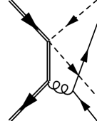
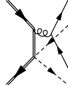
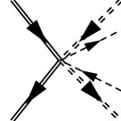
Figure 5: Matching $\text{NRQCD}+\text{SCET}$ onto $\text{pNRQCD}+\text{bHQET}$. On the r.h.s. the double solid lines represent heavy $b$ ($\bar{b}$) (anti)quarks, the double dashed lines bHQET $c$ ($\bar{c}$) (anti)quarks, and the single dashed lines collinear light quarks.

The amplitude for the decay of a bottomonium with quantum numbers ${}^{2S+1}L_{J}$ into two $D$ mesons has the following form:

$$\begin{split}i\mathcal{M}=iC(\mu)\int\frac{d\omega}{\omega}\frac{d\bar{\omega}}{\bar{\omega}}T(\omega,\bar{\omega},\mu,\mu^{\prime};^{2S+1}L_{J})F^{2}(\mu^{\prime})\langle DA,\,DB|\mathcal{O}^{{}^{2S+1}L_{J}}_{AB}(\omega,\bar{\omega},\mu^{\prime})|\bar{b}b(^{2S+1}L_{J})\rangle.\end{split}$$ (30)

$A$ and $B$, which label the final states and the $\text{EFT}_{\text{II}}$ operators $\mathcal{O}^{{}^{2S+1}L_{J}}_{AB}$, denote the possible parity, spin, and polarization of the $D$ mesons, $A,B=\{P,V_{L},V_{T}\}$, indicating respectively a pseudoscalar $D$ meson, a longitudinally-polarized vector meson $D^{*}$, and a transversely-polarized vector meson $D^{*}$. Unlike $J_{\text{EFT}_{\text{I}}}$, we have dropped the subscript $\text{EFT}_{\text{II}}$ in $\mathcal{O}^{{}^{2S+1}L_{J}}_{AB}$ in order to simplify the notation.

The $\text{EFT}_{\text{II}}$ operators that contribute to the decay of the $P$-wave states are

$$\begin{split}F^{2}(\mu^{\prime})\,\mathcal{O}^{{}^{3}P_{J}}_{PP}(\omega,\bar{\omega},\mu^{\prime})&=\chi^{\dagger}_{\bar{b}}\,\vec{p}_{b}\cdot\vec{\sigma}_{\perp}\psi_{b}\;\bar{\mathcal{H}}^{c}_{\bar{n}}\,\frac{\hbox to0.0pt{\hbox to6.00235pt{\hfil/\hfil}\hss}n}{2}\gamma^{5}\,\delta\left(-\bar{\omega}-n\cdot\mathcal{P}\right)\chi^{\bar{l}}_{\bar{n}}\;\bar{\chi}^{l}_{n}\delta\left(\omega-\bar{n}\cdot\mathcal{P}^{\dagger}\right)\,\frac{\hbox to0.0pt{\hbox to5.00002pt{\hfil/\hfil}\hss}\bar{n}}{2}\gamma^{5}\,\mathcal{H}^{\bar{c}}_{n}\;,\\ F^{2}(\mu^{\prime})\,\mathcal{O}^{{}^{3}P_{J}}_{V_{L}\,V_{L}}(\omega,\bar{\omega},\mu^{\prime})&=\chi^{\dagger}_{\bar{b}}\,\vec{p}_{b}\cdot\vec{\sigma}_{\perp}\psi_{b}\;\bar{\mathcal{H}}^{c}_{\bar{n}}\,\frac{\hbox to0.0pt{\hbox to6.00235pt{\hfil/\hfil}\hss}n}{2}\,\delta\left(-\bar{\omega}-n\cdot\mathcal{P}\right)\chi^{\bar{l}}_{\bar{n}}\;\bar{\chi}^{l}_{n}\delta\left(\omega-\bar{n}\cdot\mathcal{P}^{\dagger}\right)\,\frac{\hbox to0.0pt{\hbox to5.00002pt{\hfil/\hfil}\hss}\bar{n}}{2}\,\mathcal{H}^{\bar{c}}_{n}\;,\\ F^{2}(\mu^{\prime})\,\mathcal{O}^{{}^{3}P_{J}}_{V_{T}\,V_{T}}(\omega,\bar{\omega},\mu^{\prime})&=\chi^{\dagger}_{\bar{b}}\,{p}^{\,(\mu}_{b\,\perp}\sigma^{\nu)}_{\perp}\psi_{b}\;\bar{\mathcal{H}}^{c}_{\bar{n}}\,\frac{\hbox to0.0pt{\hbox to6.00235pt{\hfil/\hfil}\hss}n}{2}\gamma_{\mu\,\perp}\,\delta\left(-\bar{\omega}-n\cdot\mathcal{P}\right)\chi^{\bar{l}}_{\bar{n}}\;\bar{\chi}^{l}_{n}\delta\left(\omega-\bar{n}\cdot\mathcal{P}^{\dagger}\right)\,\frac{\hbox to0.0pt{\hbox to5.00002pt{\hfil/\hfil}\hss}\bar{n}}{2}\gamma_{\nu\,\perp}\,\mathcal{H}^{\bar{c}}_{n},\\ \end{split}$$ (31)

where ${p}^{\,(\mu}_{b\,\perp}\sigma^{\nu)}_{\perp}$ is a symmetric, traceless tensor,

$${p}^{\,(\mu}_{b\,\perp}\sigma^{\nu)}_{\perp}=\frac{1}{2}\left({p}^{\,\mu}_{b\,\perp}\sigma^{\nu}_{\perp}+{p}^{\,\nu}_{b\,\perp}\sigma^{\mu}_{\perp}-g^{\mu\nu}_{\perp}\vec{p}_{b}\cdot\vec{\sigma}_{\perp}\right)\;.$$

At leading order in the $\text{EFT}_{\text{II}}$ expansion, the $\eta_{b}$ can only decay into a pseudoscalar and a vector meson, with an operator given by

$$\begin{split}F^{2}(\mu^{\prime})\,\mathcal{O}^{{}^{1}S_{0}}_{P\,V_{L}}(\omega,\bar{\omega},\mu^{\prime})=\chi^{\dagger}_{\bar{b}}\,\psi_{b}\;&\left[\bar{\mathcal{H}}^{c}_{\bar{n}}\,\frac{\hbox to0.0pt{\hbox to6.00235pt{\hfil/\hfil}\hss}n}{2}\gamma^{5}\,\delta\left(-\bar{\omega}-n\cdot\mathcal{P}\right)\chi^{\bar{l}}_{\bar{n}}\;\bar{\chi}^{l}_{n}\delta\left(\omega-\bar{n}\cdot\mathcal{P}^{\dagger}\right)\,\frac{\hbox to0.0pt{\hbox to5.00002pt{\hfil/\hfil}\hss}\bar{n}}{2}\,\mathcal{H}^{\bar{c}}_{n}\right.\\ &+\left.\bar{\mathcal{H}}^{c}_{\bar{n}}\,\frac{\hbox to0.0pt{\hbox to6.00235pt{\hfil/\hfil}\hss}n}{2}\,\delta\left(-\bar{\omega}-n\cdot\mathcal{P}\right)\chi^{\bar{l}}_{\bar{n}}\;\bar{\chi}^{l}_{n}\delta\left(\omega-\bar{n}\cdot\mathcal{P}^{\dagger}\right)\,\frac{\hbox to0.0pt{\hbox to5.00002pt{\hfil/\hfil}\hss}\bar{n}}{2}\gamma^{5}\,\mathcal{H}^{\bar{c}}_{n}\right].\end{split}$$ (32)

For later convenience, in the definition of the effective operators (31) and (32) we have factored out the term $F^{2}(\mu^{\prime})$, which is related to the $D$-meson decay constant. The definition of $F^{2}(\mu^{\prime})$ will become clear when we introduce the $D$-meson distribution amplitudes. The fields $\chi^{l}_{n}$ and $\chi^{\bar{l}}_{\bar{n}}$ are ultracollinear gauge-invariant light-quark fields, while $\mathcal{H}^{c}_{\bar{n}}=W^{\dagger}_{\bar{n}}h^{c}_{\bar{n}}$ and $\mathcal{H}^{\bar{c}}_{n}=W^{\dagger}_{n}h^{\bar{c}}_{n}$ are bHQET heavy-quark fields, which are invariant under an ultracollinear gauge transformation. The Wilson lines $W_{n}$ and $W_{\bar{n}}$ have the same definition as in Eq. (8), with the restriction to ultracollinear gluons. Eqs. (31) and (32) allow us to interpret $\omega$ as the component of the light-quark momentum along the direction $n$. Similarly, $\bar{\omega}$ represents the component of the light-antiquark momentum along $\bar{n}$. The minus sign in the delta function $\delta(-\bar{\omega}-n\cdot\mathcal{P})$ is chosen so that $\bar{\omega}$ is positive.

The tree-level matching coefficients are

$$\begin{split}T(\omega,\bar{\omega},\mu,\mu^{\prime}=m_{c};\,^{3}P_{J})&=\frac{C_{F}}{N_{c}^{2}}\frac{4\pi\alpha_{s}(m_{c})}{m_{b}}\frac{1}{\omega+\bar{\omega}}\;,\\ T(\omega,\bar{\omega},\mu,\mu^{\prime}=m_{c};\,^{1}S_{0})&=\frac{C_{F}}{N_{c}^{2}}\frac{4\pi\alpha_{s}(m_{c})}{m_{b}}\frac{1}{2}\frac{\omega-\bar{\omega}}{\omega+\bar{\omega}}\;.\end{split}$$ (33)

Note that, at leading order in the $\text{EFT}_{\text{II}}$ expansion, the matching coefficient $T(\omega,\bar{\omega},\mu,\mu^{\prime};\,^{3}P_{J})$ is independent of the spin and polarization of the final states, or of the total angular momentum $J$ of the $\chi_{b}$.

An important feature of bHQET is that the ultracollinear and ultrasoft sectors can be decoupled at leading order in the power counting by a field redefinition reminiscent of the collinear-usoft decoupling in SCET Bauer:2001yt Fleming:2007qr . For bHQET in the $n$ direction, the decoupling is achieved by defining $h^{\bar{c}}_{n}\rightarrow Y_{n}h^{\bar{c}}_{n}$ and $\bar{\xi}^{l}_{n}\rightarrow\bar{\xi}^{l}_{n}Y^{\dagger}_{n}$, where $Y_{n}$ is an ultrasoft Wilson line,

$$Y_{n}=\sum_{\rm{perms}}\left[\exp\left(-\frac{g}{n\cdot\mathcal{P}}n\cdot A_{us}\right)\right]\;.$$ (34)

An analogous redefinition with $n\rightarrow\bar{n}$ decouples ultrasoft from $\bar{n}$-ultracollinear quarks and gluons. These redefinitions do not affect the operators in Eqs. (31) and (32) because all the induced Wilson lines cancel out. As a consequence, at leading order in the $\text{EFT}_{\text{II}}$ power counting, there is no interaction between the initial and the final states, since the former can only emit and absorb ultrasoft gluons that do not couple to ultracollinear degrees of freedom. Furthermore, fields in the two copies of bHQET, boosted in opposite directions, cannot interact with each other because the interaction with a $\bar{n}$-ultracollinear gluon would give a $n$-ultracollinear quark or gluon a virtuality of order $m^{2}_{c}$, which, however, cannot appear in $\text{EFT}_{\text{II}}$. The matrix elements of the operators $\mathcal{O}^{{}^{2S+1}L_{J}}_{AB}(\omega,\bar{\omega},\mu)$, therefore, factorize as

$$\begin{split}F^{2}(\mu^{\prime})\langle AB|\mathcal{O}^{{}^{2S+1}L_{J}}_{A\,B}(\omega,\bar{\omega},\mu^{\prime})|\bar{b}b\rangle=&\langle 0|\chi^{\dagger}_{\bar{b}}\,T^{{}^{2S+1}L_{J}}_{AB}\psi_{b}|\bar{b}b\rangle\,\langle A|\bar{\mathcal{H}}^{c}_{\bar{n}}\,\frac{\hbox to0.0pt{\hbox to6.00235pt{\hfil/\hfil}\hss}n}{2}\Gamma_{A}\,\delta\left(-\bar{\omega}-n\cdot\mathcal{P}\right)\chi^{\bar{l}}_{\bar{n}}|0\rangle\\ &\langle B|\bar{\chi}^{l}_{n}\delta\left(\omega-\bar{n}\cdot\mathcal{P}^{\dagger}\right)\,\frac{\hbox to0.0pt{\hbox to5.00002pt{\hfil/\hfil}\hss}\bar{n}}{2}\Gamma_{B}\,\mathcal{H}^{\bar{c}}_{n}|0\rangle\;,\end{split}$$ (35)

where $\Gamma_{A}=\{\gamma_{5},1,\gamma^{\mu}_{\perp}\}$ and $T^{{}^{2S+1}L_{J}}_{AB}=\{1,\,\vec{p}_{b}\cdot\vec{\sigma}_{\perp},\,{p}^{\,(\mu}_{b\,\perp}\sigma^{\nu)}_{\perp}\}$. The charge-conjugated contribution is understood in the $\eta_{b}$ case.

The quarkonium state and the $D$ mesons in Eq. (35) have respectively non-relativistic and HQET normalization:

$$\langle\chi_{bJ}(E^{\prime},\vec{p}^{\,\prime})|\chi_{bJ}(E,\vec{p})\rangle=(2\pi)^{3}\delta^{(3)}(\vec{p}-\vec{p}^{\,\prime})\;,\quad\langle D(v^{\prime},k^{\prime})|D(v,k)\rangle=2v^{0}\delta_{v,v^{\prime}}(2\pi)^{3}\delta^{(3)}(\vec{k}-\vec{k}^{\prime})\;,$$

where $v^{0}$ is the 0th component of the 4-velocity $v^{\mu}$.

The $D$-meson matrix elements can be expressed in terms of the $D$-meson light-cone distribution amplitudes:

$$\langle P|\bar{\chi}^{l}_{n}\,\frac{\hbox to0.0pt{\hbox to5.00002pt{\hfil/\hfil}\hss}\bar{n}}{2}\gamma^{5}\,\delta\left({\omega}-\bar{n}\cdot\mathcal{P}^{\dagger}\right){\mathcal{H}}^{\bar{c}}_{n}|0\rangle =iF_{P}(\mu^{\prime})\frac{\bar{n}\cdot v}{2}\phi_{P}({\omega},\mu^{\prime})\;,$$ (36)

$$\langle V_{L}|\bar{\chi}^{l}_{n}\,\frac{\hbox to0.0pt{\hbox to5.00002pt{\hfil/\hfil}\hss}\bar{n}}{2}\,\delta\left({\omega}-\bar{n}\cdot\mathcal{P}^{\dagger}\right){\mathcal{H}}^{\bar{c}}_{n}|0\rangle =F_{V_{L}}(\mu^{\prime})\frac{\bar{n}\cdot v}{2}\phi_{V_{L}}({\omega},\mu^{\prime})\;,$$ (37)

$$\langle V_{T}|\bar{\chi}^{l}_{n}\,\frac{\hbox to0.0pt{\hbox to5.00002pt{\hfil/\hfil}\hss}\bar{n}}{2}\gamma^{\mu}_{\perp}\,\delta\left({\omega}-\bar{n}\cdot\mathcal{P}^{\dagger}\right){\mathcal{H}}^{\bar{c}}_{n}|0\rangle =F_{V_{T}}(\mu^{\prime})\frac{\bar{n}\cdot v}{2}\varepsilon^{\mu}_{\perp}\phi_{V_{T}}({\omega},\mu^{\prime})\;,$$ (38)

where $\varepsilon^{\mu}_{\perp}$ is the transverse polarization of the vector meson. The constants $F_{A}(\mu^{\prime})$, with $A=\{P,V_{L},V_{T}\}$, are related to the matrix elements of the local heavy-light currents in coordinate space. In the heavy-quark limit, where $D$ and $D^{*}$ are degenerate, $F_{A}$ is the same for all the three states: $F\equiv F_{P}=F_{V_{L}}=F_{V_{T}}$. In this limit,

$$\langle 0|\bar{\xi}^{\,\bar{l}}_{n}\,\frac{\hbox to0.0pt{\hbox to5.00002pt{\hfil/\hfil}\hss}\bar{n}}{2}\gamma^{5}{h}^{c}_{n}(0)|P\rangle=-iF(\mu^{\prime})\frac{\bar{n}\cdot v^{\prime}}{2}\;.$$ (39)

At tree level, the matrix element is proportional to the $D$-meson decay constant $f_{D}=205.8\pm 8.5\pm 2.5$ MeV :2008sq . More precisely, $F(\mu^{\prime})=f_{D}\sqrt{m_{D}}$, where the factor $\sqrt{m_{D}}$ is due to HQET normalization. The scale dependence of $F$ is determined by the renormalization of heavy-light HQET currents. At one loop, Ref. Manohar showed that

$$\frac{d}{d\ln\mu^{\prime}}F(\mu^{\prime})=-\gamma_{F}F(\mu^{\prime})=3C_{F}\frac{\alpha_{s}}{4\pi}F(\mu^{\prime})\;.$$ (40)

The pNRQCD matrix elements can be expressed in terms of the heavy quarkonium wavefunctions. The operator $\chi^{\dagger}_{\bar{b}}\vec{p}_{b}\cdot\vec{\sigma}_{\perp}\psi_{b}$ contains a component with $J=0$ and a component with $J=2$ and $J_{z}=0$, so its matrix element has non-vanishing overlap with both $\chi_{b0}$ and $\chi_{b2}$. The operator $\chi^{\dagger}_{\bar{b}}p^{\,(\mu}_{b}{\sigma}^{\,\nu)}_{\perp}\psi_{b}$ instead has only contributions with $J=2$ and $J_{z}=\pm 2$ and therefore it only overlaps with $\chi_{b2}$. In terms of the bottomonium wavefunctions, the pNRQCD matrix elements are expressed as

$$\langle 0|\chi^{\dagger}_{\bar{b}}\vec{p}_{b}\cdot\vec{\sigma}_{\perp}\psi_{b}|\chi_{b0}\rangle =\frac{2}{\sqrt{3}}\,\sqrt{\frac{3N_{c}}{2\pi}}R^{\prime}_{\chi_{b0}}(0,\mu^{\prime})\;,$$ (41)

$$\langle 0|\chi^{\dagger}_{\bar{b}}\vec{p}_{b}\cdot\vec{\sigma}_{\perp}\psi_{b}|\chi_{b2}\rangle =-\sqrt{\frac{2}{15}}\,\sqrt{\frac{3N_{c}}{2\pi}}R^{\prime}_{\chi_{b2}}(0,\mu^{\prime})\;,$$ (42)

$$\langle 0|\chi^{\dagger}_{\bar{b}}p^{\,(\mu}_{b}{\sigma}^{\,\nu)}_{\perp}\psi_{b}|\chi_{b2}\rangle =(\varepsilon^{(2)}_{\mu\nu}+\varepsilon^{(-2)}_{\mu\nu})\,\sqrt{\frac{3N_{c}}{2\pi}}R^{\prime}_{\chi_{b2}}(0,\mu^{\prime})\;,$$ (43)

where $R^{\prime}_{\chi_{bJ}}(0)$ is the derivative of the radial wavefunction of the $\chi_{bJ}$ evaluated at the origin. At leading order, the pNRQCD Hamiltonian does not depend on $J$, so, up to corrections of order $w^{2}$, $R^{\prime}_{\chi_{b2}}(0)=R^{\prime}_{\chi_{b0}}(0)$. The numerical pre-factors in Eqs. (41) and (42) follow from decomposing $\vec{p}_{b}\cdot\vec{\sigma}_{\perp}$ into components with definite $J_{z}$. $\varepsilon^{(j)}_{\mu\nu}$ is the polarization tensor of the $\chi_{b2}$ state, and Eq. (43) states that, at leading order in the $w^{2}$ expansion, only the particles with polarization $J_{z}=\pm 2$ contribute to $\chi_{b2}$ decay into two transversely-polarized vector mesons. Similarly, one finds

$$\langle 0|\chi^{\dagger}_{\bar{b}}\psi_{b}|\eta_{b}\rangle=\sqrt{\frac{N_{c}}{2\pi}}R_{\eta_{b}}(0,\mu^{\prime})\;.$$ (44)

The factorization of the matrix elements (35) implies that the decay rate also factorizes. For the decays of $\chi_{b0}$ and $\chi_{b2}$ into two pseudoscalar mesons or two longitudinally-polarized vector mesons, we find

$$\begin{split}\Gamma\left(\chi_{b0}\rightarrow AA\right)=&\frac{4}{3}\frac{m^{2}_{D}\sqrt{m^{2}_{\chi_{b0}}-4m^{2}_{D}}}{8\pi m_{\chi_{b0}}}\frac{3N_{c}}{2\pi}\,|C\left(\mu\right)|^{2}\,|R^{\prime}_{\chi_{b0}}(0,\mu^{\prime})|^{2}\\ &\left[F^{2}(\mu^{\prime})\frac{n\cdot v^{\prime}}{2}\frac{\bar{n}\cdot v}{2}\int\frac{d\omega}{\omega}\frac{d\bar{\omega}}{\bar{\omega}}T\left(\omega,\bar{\omega},\mu,\mu^{\prime};\,^{3}P_{J}\right)\phi_{A}(\bar{\omega},\mu^{\prime})\phi_{A}(\omega,\mu^{\prime})\right]^{2}\end{split}$$ (45)

and

$$\begin{split}\Gamma\left(\chi_{b2}\rightarrow AA\right)=&\frac{2}{15}\frac{m^{2}_{D}\sqrt{m^{2}_{\chi_{b2}}-4m^{2}_{D}}}{8\pi m_{\chi_{b2}}}\frac{3N_{c}}{2\pi}|C\left(\mu\right)|^{2}\,|R^{\prime}_{\chi_{b2}}(0,\mu^{\prime})|^{2}\\ &\left[F^{2}(\mu^{\prime})\frac{n\cdot v^{\prime}}{2}\frac{\bar{n}\cdot v}{2}\int\frac{d\omega}{\omega}\frac{d\bar{\omega}}{\bar{\omega}}T\left(\omega,\bar{\omega},\mu,\mu^{\prime};\,^{3}P_{J}\right)\phi_{A}(\bar{\omega},\mu^{\prime})\phi_{A}(\omega,\mu^{\prime})\right]^{2}\;,\end{split}$$ (46)

where $A=P,V_{L}$. For the decay of $\chi_{b2}$ into two transversely-polarized vector mesons, one finds the decay rate by summing over the possible transverse polarizations:

$$\begin{split}\Gamma\left(\chi_{b2}\rightarrow V_{T}V_{T}\right)=&\frac{2}{5}\frac{m^{2}_{D}\sqrt{m^{2}_{\chi_{b2}}-4m^{2}_{D}}}{8\pi m_{\chi_{b2}}}\frac{3N_{c}}{2\pi}|C\left(\mu\right)|^{2}\,\,|R^{\prime}_{\chi_{b2}}(0,\mu^{\prime})|^{2}\\ &\left[F^{2}(\mu^{\prime})\frac{n\cdot v^{\prime}}{2}\frac{\bar{n}\cdot v}{2}\int\frac{d\omega}{\omega}\frac{d\bar{\omega}}{\bar{\omega}}T\left(\omega,\bar{\omega},\mu,\mu^{\prime};\,^{3}P_{J}\right)\phi_{V_{T}}(\bar{\omega},\mu^{\prime})\phi_{V_{T}}(\omega,\mu^{\prime})\right]^{2}\;.\end{split}$$ (47)

In the case of $\eta_{b}$ decay into a pseudoscalar and a longitudinally-polarized vector meson, we find

$$\begin{split}\Gamma\left(\eta_{b}\rightarrow PV_{L}+\rm{c.c.}\right)=\frac{m^{2}_{D}\sqrt{m^{2}_{\eta_{b}}-4m^{2}_{D}}}{8\pi m_{\eta_{b}}}\frac{N_{c}}{2\pi}|C\left(\mu\right)|^{2}\,\,|R_{\eta_{b}}(0,\mu^{\prime})|^{2}\,\frac{1}{2}\left[F^{2}(\mu^{\prime})\frac{n\cdot v^{\prime}}{2}\frac{\bar{n}\cdot v}{2}\right.&\\ \left.\int\frac{d\omega}{\omega}\frac{d\bar{\omega}}{\bar{\omega}}T\left(\omega,\bar{\omega},\mu,\mu^{\prime};\,^{1}S_{0}\right)(\phi_{V_{L}}(\bar{\omega},\mu^{\prime})\phi_{P}(\omega,\mu^{\prime})-\phi_{V_{L}}(\omega,\mu^{\prime})\phi_{P}(\bar{\omega},\mu^{\prime}))\right]^{2}&.\end{split}$$ (48)

Note that we are working in the limit $m_{c}\to\infty$, where the $m_{D^{*}}-m_{D}$ mass splitting vanishes.

The factorized formulas Eqs. (35) and (45) - (48) are the main results of this paper. Each decay rate of (45) - (48) depends on two calculable matching coefficients, $C$ and $T$, and three non-perturbative, process-independent matrix elements, namely, two $D$-meson distribution amplitudes and the bottomonium wavefunction. In Sec. V we will provide a model-dependent estimate of the decay rates (45) - (48) and will discuss the phenomenological implications. We conclude this section by observing that all the non-perturbative matrix elements cancel out in the ratios $\Gamma(\chi_{b0}\rightarrow PP)/\Gamma(\chi_{b2}\rightarrow PP)$ and $\Gamma(\chi_{b0}\rightarrow V_{L}V_{L})/\Gamma(\chi_{b2}\rightarrow V_{L}V_{L})$, since the spin symmetry of pNRQCD guarantees $R^{\prime}_{\chi_{b0}}(0)=R^{\prime}_{\chi_{b2}}(0)$, at leading order in $\text{EFT}_{\text{II}}$. Neglecting the $\chi_{b0}$ - $\chi_{b2}$ mass difference, we find, up to corrections of order $w^{2}$,

$$\Gamma(\chi_{b0}\rightarrow AA)/\Gamma(\chi_{b2}\rightarrow AA)=\frac{4}{3}\frac{15}{2}=10\;,$$ (49)

with $A=P,V_{L}$.

IV.2 Running

The dependence of the matching coefficient $T(\omega,\bar{\omega},\mu,\mu^{\prime};\,^{2S+1}L_{J})$ and of the operators in Eqs. (45) - (48) on the scale $\mu^{\prime}$ is driven by a RGE that can be obtained by renormalizing the $\text{EFT}_{\text{II}}$ operators. The RGE for the $\text{EFT}_{\text{II}}$ operators, which also defines the anomalous dimension $\gamma_{\text{EFT}_{\text{II}}}$, is similar to Eq. (10),

$$\begin{split}\frac{d}{d\ln\mu^{\prime}}&\left[F^{2}(\mu^{\prime})\mathcal{O}^{{}^{2S+1}L_{J}}_{AB}\left(\omega,\bar{\omega},\mu^{\prime}\right)\right]=\\ &\hskip 71.13188pt-\int d\omega^{\prime}\int d\bar{\omega}^{\prime}\gamma_{\text{EFT}_{\text{II}}}(\omega,\omega^{\prime};\bar{\omega},\bar{\omega}^{\prime};\mu^{\prime})F^{2}(\mu^{\prime})\mathcal{O}^{{}^{2S+1}L_{J}}_{AB}(\omega^{\prime},\bar{\omega}^{\prime},\mu^{\prime})\;.\end{split}$$ (50)

To calculate the anomalous dimension at one loop, we compute the divergent part of the diagrams in Figs. 6 and 7. As mentioned in Sec. II, the pNRQCD Lagrangian has the following structure,

$$L_{\rm{pNRQCD}}=\int d^{3}x\,\mathcal{L}^{usoft}_{\rm{NRQCD}}+L_{\rm{pot}}\;,$$

where the superscript $usoft$ indicates that the gluons in the NRQCD Lagrangian are purely ultrasoft ($m_{b}w^{2},m_{b}w^{2}$), while $L_{\rm{pot}}$ contains four-fermions operators, which are non-local in space,

$$L_{\rm{pot}}=\int d^{3}x_{1}d^{3}x_{2}\psi^{\dagger}_{\alpha}(t,\vec{x}_{1})\chi_{\beta}(t,\vec{x}_{2})V_{\alpha\beta,\gamma\delta}(\vec{r}\,)\chi^{\dagger}_{\gamma}(t,\vec{x}_{2})\psi_{\delta}(t,\vec{x}_{1})\;.$$

At leading order in $\alpha_{s}(m_{b}w)$ and $r$, $V$ is the Coulomb potential

$$V_{\alpha\beta,\gamma\delta}=\frac{\alpha_{s}(m_{b}w)}{r}t^{a}_{\alpha\delta}t^{a}_{\gamma\beta}\;.$$

For the explicit form of higher-order potentials, see, for example, Refs. Brambilla:2004jw Hoang:2002yy . Vertices from $L_{\rm{pot}}$ generate one-loop diagrams as the first diagram in Fig. 6. However, these diagrams do not give any contribution to the anomalous dimension at one loop. Indeed, the insertion of the Coulomb potential $1/r$ in Fig. 6 does not produce UV divergences. Insertions of the $1/m_{b}$ potentials yield divergences but the coefficient of the $1/m_{b}$ potential is proportional to $\alpha_{s}^{2}(m_{b}w)$, so it is not relevant if we are content with a NLL resummation. Insertions of $1/m^{2}_{b}$ potentials give divergences proportional to subleading operators, which can be neglected. The second diagram in Fig. 6 yields a result completely analogous to the last term in Eq. (13), with the only difference of a color pre-factor,

$$i\mathcal{M}_{\rm{pNRQCD}}=-i\frac{\alpha_{s}}{2\pi}\,\frac{C_{F}}{\varepsilon}\mathcal{O}^{{}^{2S+1}L_{J}}_{AB}(\omega,\bar{\omega},\mu)\;.$$ (51)

This divergence is completely cancelled by the $b$-quark field renormalization constant $Z_{b}$, and hence the pNRQCD diagrams in Fig. 6 do not contribute to the anomalous dimension at one loop.

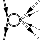
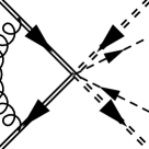
Figure 6: One-loop diagrams in pNRQCD. The first diagram contains insertions of quark-antiquark potentials. In the second diagram the gluon is ultrasoft.

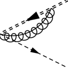
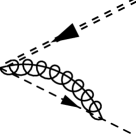
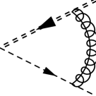
Figure 7: One-loop diagrams in bHQET. There are three analogous diagrams for the other copy of bHQET.

On the bHQET side, the third diagram in Fig. 7 is convergent, and hence it does not contribute to the anomalous dimension. The first two diagrams give

$$i\mathcal{M}_{\rm{bHQET},\bar{n}}=i\int d\omega^{\prime}d\bar{\omega}^{\prime}\Delta(\omega,\omega^{\prime},\,\bar{\omega},\bar{\omega}^{\prime})\mathcal{O}^{{}^{2S+1}L_{J}}_{AB}(\omega^{\prime},\bar{\omega}^{\prime},\mu)\;,$$ (52)

with

$$\begin{split}\Delta(\omega,\omega^{\prime},\,\bar{\omega},\bar{\omega}^{\prime})=&\frac{\alpha_{s}}{2\pi}C_{F}\delta(\omega-\omega^{\prime})\left\{\delta\left(\bar{\omega}-\bar{\omega}^{\prime}\right)\left[-\frac{1}{2\varepsilon^{2}}-\frac{1}{\varepsilon}\ln\left(\frac{\mu^{\prime}n\cdot v^{\prime}}{\bar{\omega}^{\prime}}\right)+\frac{1}{\varepsilon}\right]\right.\\ &+\left.\frac{1}{\varepsilon}\left[\theta\left(\bar{\omega}-\bar{\omega}^{\prime}\right)\left(\frac{1}{\bar{\omega}-\bar{\omega}^{\prime}}\right)_{+}+\theta\left(\bar{\omega}^{\prime}-\bar{\omega}\right)\theta\left(\bar{\omega}\right)\frac{\bar{\omega}}{\bar{\omega}^{\prime}}\left(\frac{1}{\bar{\omega}^{\prime}-\bar{\omega}}\right)_{+}\right]\right\}\;.\end{split}$$ (53)

The diagrams for the bHQET copy in the $n$-direction give a result analogous to Eqs. (52) and (53), with $\bar{\omega}\rightarrow\omega$, $\bar{\omega}^{\prime}\rightarrow\omega^{\prime}$, and $n\cdot v^{\,\prime}\rightarrow\bar{n}\cdot v$. Extracting $\gamma_{\text{EFT}_{\text{II}}}$ from the divergence is again standard, just as we did in the case of $\gamma_{\text{EFT}_{\text{I}}}$. After adding to Eq. (53) the bHQET field renormalization constants $Z_{h}$ and $Z_{\xi}$ for heavy and light quarks

$$Z_{h}=1+\frac{1}{\varepsilon}\frac{\alpha_{s}}{2\pi}C_{F}\;,\qquad Z_{\xi}=1-\frac{1}{\varepsilon}\frac{\alpha_{s}}{4\pi}C_{F}\;,$$

we find

$$\begin{split}\gamma_{\text{EFT}_{\text{II}}}(\omega,\omega^{\prime};\bar{\omega},\bar{\omega}^{\prime};\mu^{\prime})=2\gamma_{F}\,\delta\left(\omega-\omega^{\prime}\right)\delta\left(\bar{\omega}-\bar{\omega}^{\prime}\right)+\gamma_{\mathcal{O}}(\omega,\omega^{\prime};\bar{\omega},\bar{\omega}^{\prime};\mu^{\prime})\;,\end{split}$$ (54)

with

$$\begin{split}&\gamma_{\mathcal{O}}(\omega,\omega^{\prime};\bar{\omega},\bar{\omega}^{\prime};\mu^{\prime})\\ &=\frac{\alpha_{s}}{4\pi}\,4C_{F}\delta\left(\omega-\omega^{\prime}\right)\delta\left(\bar{\omega}-\bar{\omega}^{\prime}\right)\left[-1+\ln\left(\frac{{\mu}^{\prime}n\cdot v^{\prime}}{\bar{\omega}^{\prime}}\right)+\ln\left(\frac{{\mu}^{\prime}\bar{n}\cdot v}{{\omega}^{\prime}}\right)\right]\\ &-\frac{\alpha_{s}}{4\pi}4C_{F}\delta\left(\omega-\omega^{\prime}\right)\left[\theta\left(\bar{\omega}-\bar{\omega}^{\prime}\right)\left(\frac{1}{\bar{\omega}-\bar{\omega}^{\prime}}\right)_{+}+\theta\left(\bar{\omega}^{\prime}-\bar{\omega}\right)\theta\left(\bar{\omega}\right)\frac{\bar{\omega}}{\bar{\omega}^{\prime}}\left(\frac{1}{\bar{\omega}^{\prime}-\bar{\omega}}\right)_{+}\right]\\ &-\frac{\alpha_{s}}{4\pi}4C_{F}\delta\left(\bar{\omega}-\bar{\omega}^{\prime}\right)\left[\theta\left({\omega}-{\omega}^{\prime}\right)\left(\frac{1}{{\omega}-{\omega}^{\prime}}\right)_{+}+\theta\left({\omega}^{\prime}-{\omega}\right)\theta\left({\omega}\right)\frac{{\omega}}{{\omega}^{\prime}}\left(\frac{1}{{\omega}^{\prime}-{\omega}}\right)_{+}\right]\;.\end{split}$$ (55)

The term proportional to $\gamma_{F}$ in Eq. (54) reproduces the running of $F^{2}(\mu^{\prime})$ (40). $\gamma_{\mathcal{O}}$ is responsible for the running of the $D$-meson distribution amplitudes and it agrees with the result found in Ref. Lange:2003ff . Also, in Eq. (55) the coefficient of $\ln\mu^{\prime}$ is proportional to $\Gamma_{\rm{cusp}}(\alpha_{s})$. Note that, since the bHQET Lagrangian is spin-independent, the anomalous dimension does not depend on the spin or on the polarization of the $D$ meson in the final state, at leading order in the power counting.

Using Eqs. (50) and (54) we find the following integro-differential RGE for the operator $\mathcal{O}(\omega,\bar{\omega},\mu^{\prime})$:

$$\frac{d}{d\ln\mu^{\prime}}\mathcal{O}(\omega,\bar{\omega},\mu^{\prime})=-\int d\omega^{\prime}\int d\bar{\omega}^{\prime}\gamma_{\mathcal{O}}(\omega,\omega^{\prime};\bar{\omega},\bar{\omega}^{\prime};\mu^{\prime})\mathcal{O}(\omega^{\prime},\bar{\omega}^{\prime},\mu^{\prime})\;,$$ (56)

where we have dropped both the subscripts $A$, $B$, and the superscript ${}^{2S+1}L_{J}$, since $\gamma_{\mathcal{O}}$ does not depend on the quantum numbers of the initial or final state. Using the fact that the convolution of $F^{2}(\mu^{\prime})\,T(\omega,\bar{\omega},\mu,\mu^{\prime};\,^{2S+1}L_{J})$ and the operator $\mathcal{O}^{{}^{2S+1}L_{J}}_{AB}(\omega,\bar{\omega},\mu^{\prime})$ is $\mu^{\prime}$-independent, we can write an equation for the coefficient,

$$\begin{split}\frac{d}{d\ln\mu^{\prime}}\left[F^{2}(\mu^{\prime})\,T(\omega,\bar{\omega},\mu,\mu^{\prime})\right]&=\int d\omega^{\prime}\int d\bar{\omega}^{\prime}\frac{\omega}{\omega^{\prime}}\frac{\bar{\omega}}{\bar{\omega}^{\prime}}F^{2}(\mu^{\prime})\,T(\omega^{\prime},\bar{\omega}^{\prime},\mu,\mu^{\prime})\gamma_{\mathcal{O}}(\omega^{\prime},\omega;\bar{\omega}^{\prime},\bar{\omega};\mu^{\prime})\\ &=\int d\omega^{\prime}\int d\bar{\omega}^{\prime}F^{2}(\mu^{\prime})\,T(\omega^{\prime},\bar{\omega}^{\prime},\mu,\mu^{\prime})\gamma_{\mathcal{O}}(\omega,\omega^{\prime};\bar{\omega},\bar{\omega}^{\prime};\mu^{\prime})\;,\end{split}$$ (57)

where the last line follows from the property of $\gamma_{\mathcal{O}}$ at one loop,

$$\frac{\omega}{\omega^{\prime}}\frac{\bar{\omega}}{\bar{\omega}^{\prime}}\gamma_{\mathcal{O}}(\omega^{\prime},\omega;\bar{\omega}^{\prime},\bar{\omega};\mu^{\prime})=\gamma_{\mathcal{O}}(\omega,\omega^{\prime};\bar{\omega},\bar{\omega}^{\prime};\mu^{\prime})\;,$$

as can be explicitly verified from the expression in Eq. (55).

Eq. (57) can be solved following the methods described in Ref. Lange:2003ff . We discuss the details of the solution in App. A, where we derive the analytic expressions for $T(\omega,\bar{\omega},\mu,\mu^{\prime};\,^{3}P_{J})$ and $T(\omega,\bar{\omega},\mu,\mu^{\prime};\,^{1}S_{0})$, with the initial conditions at the scale $\mu^{\prime}_{c}=m_{c}$ expressed in Eq. (33).

V Decay Rates and Phenomenology

In Sec. IV.1 we gave the factorized expressions for the decay rates (45) - (48): $\Gamma(\chi_{b0,\,2}\rightarrow PP)$, $\Gamma(\chi_{b0,\,2}\rightarrow V_{L}V_{L})$, $\Gamma(\chi_{b2}\rightarrow V_{T}V_{T})$, and $\Gamma(\eta_{b}\rightarrow PV_{L}+\rm{c.c.})$. In Secs. III.2 and IV.2 we exploited the RGEs (12) and (57) to run the scales $\mu$ and $\mu^{\prime}$, respectively, from the matching scales $\mu=2m_{b}$ and $\mu^{\prime}=m_{c}$ to the natural scales that contribute to the matrix elements, $\mu=m_{c}$ and $\mu^{\prime}\sim 1$ GeV, resumming in this way Sudakov logarithms of the ratios $m_{c}/2m_{b}$ and $m_{c}/1$ GeV.

We proceed now to estimate the decay rates (45) - (48). In order to do so, we need to evaluate the following ingredients: the light-cone distribution amplitudes of the $D$ meson and of the longitudinally- and transversely-polarized $D^{*}$ mesons, and the wavefunctions of the states $\eta_{b}$ and $\chi_{bJ}$. In principle, these non-perturbative objects could be extracted from other $\eta_{b}$, $\chi_{b}$, and $D$-meson observables. In the case of the $\eta_{b}$, the value of the wavefunction at the origin can be obtained from a measurement of the inclusive hadronic width or of the decay rate for the electromagnetic process $\eta_{b}\rightarrow\gamma\gamma$, since they are both proportional to $|R_{\eta_{b}}(0)|^{2}$. Unfortunately, at the moment there are not sufficient data on $\eta_{b}$ decays. Another way to proceed is to use the spin symmetry of the leading-order pNRQCD Hamiltonian, which implies $R_{\eta_{b}}(0)=R_{\Upsilon}(0)$, and to extract the Upsilon wavefunction from $\Gamma(\Upsilon\rightarrow e^{+}e^{-})=1.28\pm 0.07$ KeV Amsler:2008zz . Using the leading-order expression for $\Gamma(\Upsilon\rightarrow e^{+}e^{-})$ Barbieri:1975ki , one finds $|R_{\Upsilon}(0)|^{2}=6.92\pm 0.38\,\rm{GeV}^{3}$, where the error only includes the experimental uncertainty. The above value is in good agreement with the lattice evaluation by Bodwin, Sinclair, and Kim Bodwin:2001mk and it falls within the range of values obtained with four different potential models, as listed in Ref. Eichten:1995ch .

$|R^{\prime}_{\chi_{b0,\,2}}(0)|^{2}$ can be obtained from the electromagnetic decay $\chi_{b0,2}\rightarrow\gamma\gamma$. Unfortunately, such decay rates have not been measured yet. The values listed in Ref. Eichten:1995ch range from a minimum of $|R^{\prime}_{\chi_{bJ}}(0)|^{2}=1.417$ GeV⁵, obtained with the Buchmuller-Tye potential Buchmuller:1980su , to a maximum of $|R^{\prime}_{\chi_{bJ}}(0)|^{2}=2.067$ GeV⁵, obtained with a Coulomb-plus-linear potential. The lattice value is roughly of the same size, $|R^{\prime}_{\chi_{bJ}}(0)|^{2}=2.3\;\rm{GeV}^{5}$, with an uncertainty of about 15% Bodwin:2001mk . We use this value in our estimate.

For the pseudoscalar $D$-meson distribution amplitude we use two model functions widely adopted in the study of $B$ physics. A first possible choice, suggested for example in Ref. Lange:2003ff , is a simple exponential decay:

$$\phi^{\rm{Exp}}_{P,0}(\omega,\mu^{\prime}=1\rm{GeV})=\theta(\omega)\frac{\omega}{\lambda^{2}_{D}}\exp\left(-\frac{\omega}{\lambda_{D}}\right)\;.$$ (58)

Another form, suggested in Ref. Braun:2003wx , is

$$\phi^{\textrm{Braun}}_{P,\,0}(\omega,\mu^{\prime}=1\,\textrm{GeV})=\theta(\tilde{\omega})\frac{4}{\lambda_{D}\pi}\frac{\tilde{\omega}}{1+\tilde{\omega}^{2}}\left[\frac{1}{1+\tilde{\omega}^{2}}-\frac{2(\sigma_{D}-1)}{\pi^{2}}\ln\tilde{\omega}\right]\;,$$ (59)

where $\tilde{\omega}=\omega/\mu^{\prime}$. The theta function in Eqs. (58) and (59) reflects the fact that the distribution amplitudes $\phi_{A}(\omega,\mu^{\prime})$, with $A=\{P,V_{L},V_{T}\}$, have support on $\omega>0$ Grozin:1996pq .

The subscript $0$ indicates that these functional forms are valid in the $D$-meson rest frame, with a HQET velocity-label $v_{0}=(1,0,0,0)$. With the definition we adopt in Eq. (36), the distribution amplitude is not boost-invariant and in the bottomonium rest frame, in which the $D$ meson has a velocity $(n\cdot v,\bar{n}\cdot v,0)\sim(m_{c}/2m_{b},2m_{b}/m_{c},0)$, it becomes

$$\phi_{P}(\omega,\mu^{\prime})=\frac{1}{\bar{n}\cdot v}\phi_{P,\,0}\left(\frac{\omega}{\bar{n}\cdot v},\mu^{\prime}\right)\;,$$ (60)

as shown in App. B. $\lambda_{D}$ and $\sigma_{D}$ in Eqs. (58) and (59) are, respectively, the first inverse moment and the first logarithmic moment of the $D$-meson distribution amplitude in the $D$-meson rest frame,

$$\lambda_{D}^{-1}(\mu^{\prime})=\int_{0}^{\infty}\frac{d\omega}{\omega}\phi_{P,0}(\omega,\mu^{\prime})\;,$$

$$\sigma_{D}(\mu^{\prime})\lambda_{D}^{-1}(\mu^{\prime})=-\int_{0}^{\infty}\frac{d\omega}{\omega}\ln\left(\frac{\omega}{\mu^{\prime}}\right)\phi_{P,0}(\omega,\mu^{\prime})\;.$$

Furthermore we assume that the vector-meson distribution amplitudes $\phi_{V_{L}}(\omega)$ and $\phi_{V_{T}}(\omega)$ have the same functional form as $\phi_{P}(\omega)$, but with different parameters $\lambda_{D^{*}_{L}}$, $\sigma_{D^{*}_{L}}$ and $\lambda_{D^{*}_{T}}$, $\sigma_{D^{*}_{T}}$.

The $D$-meson distribution amplitude and its moments have not been intensively studied unlike, for example, the $B$-meson distribution amplitude. Therefore, we invoke heavy-quark symmetry and use the moments of the $B$-meson distribution amplitude in order to estimate the decay rate. However, the value of $\lambda_{B}$ is affected by a noticeable uncertainty. Using QCD sum rules, Braun et al. estimated Braun:2003wx $\lambda_{B}(\mu^{\prime}=1\,\rm{GeV})=0.460\pm 0.110\,\,\textrm{GeV}$, where the uncertainty is about $25\%$. Other authors Beneke:1999br Lee:2005gza Pilipp:2007sb give slightly different central values and comparable uncertainties, so that $\lambda_{B}$ falls in the range $0.350\;\textrm{GeV}<\lambda_{B}<0.600$ GeV. The first logarithmic moment $\sigma_{D}$ is given in Ref. Braun:2003wx , $\sigma_{D}=\sigma_{B}(\mu^{\prime}=1\,\rm{GeV})=1.4\pm 0.4$. We assume that the moments of the $D^{*}$-meson distribution amplitudes fall in the same range as the moments of $\phi_{P}(\omega)$.

We evaluate numerically the convolution integrals in Eqs. (45) - (48). We choose the matching scales $\mu_{b}$ and $\mu_{c}^{\prime}$ to be $2m_{b}$ and $m_{c}$ respectively. Using the RGEs we run the matching coefficients down to the scales $\mu=m_{c}$ and $\mu^{\prime}=1$ GeV. For the $b$ and $c$ quark masses we adopt the 1S mass definition Hoang:1998ng ,

$$\begin{split}m_{b}(1S)&=\frac{m_{\Upsilon}}{2}=4730.15\pm 0.13\,\,\textrm{MeV}\;,\\ m_{c}(1S)&=\frac{m_{J/\psi}}{2}=1548.46\pm 0.01\,\,\textrm{MeV}\;.\end{split}$$ (61)

The values of $\alpha_{s}$ at the relevant scales are Amsler:2008zz $\alpha_{s}(2m_{b})=0.178\pm 0.005$, $\alpha_{s}(m_{c})=0.340\pm 0.020$, and $\alpha_{s}(1\,\rm{GeV})\sim 0.5$. With these choices, the value of $g$ in Eq. (69) is $g(m_{c},1\,\rm{GeV})=-0.12\pm 0.02$.

The decay rates $\Gamma(\chi_{bJ}\rightarrow AA)$ with $A=\{P,V_{L},V_{T}\}$, (45) - (47), depend on the masses of the $\chi_{bJ}$ and of the $D$ mesons, whose most recent values are reported in Ref. Amsler:2008zz . Since the effects due to the mass splitting of the $\chi_{bJ}$ and $D$ multiplets are subleading in the EFT power counting, we use in the evaluation the average mass of the $\chi_{bJ}$ multiplet and the average mass of $D$ and $D^{*}$ mesons: $m_{\chi_{bJ}}=9898.87\pm 0.28\pm 0.31$ MeV and $m_{D}=1973.27\pm 0.18$ MeV. Therefore, the velocity of the $D$ mesons in $\chi_{bJ}$ decay is $\bar{n}\cdot v=n\cdot v^{\prime}=m_{\chi_{bJ}}/m_{D}=5.02$, with negligible error. The decay rate $\Gamma(\eta_{b}\rightarrow PV_{L}+\rm{c.c.})$ (48) depends on the mass of the $\eta_{b}$, which has been recently measured: $m_{\eta_{b}}=9388.9^{+3.1}_{-2.3}\pm 2.7$ MeV :2008vj . The velocity of the $D$ meson in the $\eta_{b}$ decay is $\bar{n}\cdot v=n\cdot v^{\prime}=m_{\eta_{b}}/m_{D}=4.76$, again with negligible error.

The decay rate $\Gamma(\chi_{b0}\rightarrow PP)$ (45), obtained with $\phi^{\rm{Exp}}$ and $\phi^{\rm{Braun}}$ separately, is shown in Fig. 8. In order to see the impact of resumming Sudakov logarithms, we show for both distribution amplitudes the results with (i) the LL and NLL resummations and (ii) without any resummation at all. In the plots, we call the resummed results NLL-resummed, indicating that Sudakov logarithms are resummed up to NLL. For both distribution amplitudes the resummation does have a relevant effect on the decay rate. In the case of $\phi^{\rm{Exp}}$ the resummation decreases the decay rate by a factor of $2-1.5$ as $\lambda_{D}$ goes from the lowest to the highest value under consideration. In the case of $\phi^{\rm{Braun}}$ the decay rate decreases too, for example, by a factor 1.5 when $\sigma_{D}=1.4$. In Fig. 9 we compare the decay rates obtained with the two distribution amplitudes. Over the range of $\lambda_{D}$ we are considering the two decay rates are in rough agreement with each other.

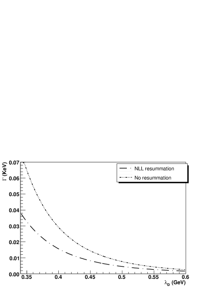
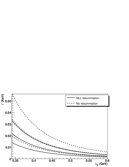
Figure 8: $\Gamma(\chi_{b0}\rightarrow PP)$ as a function of $\lambda_{D}$, calculated with the distribution amplitudes $\phi^{\textrm{Exp}}$ (left) and $\phi^{\textrm{Braun}}$ (right). The dash dotted and solid lines denote the NLL-resummed decay rate. For comparison, the decay rate without resummation is also shown, denoted by dash double-dotted (left) and dashed (right) lines. For $\phi^{\textrm{Braun}}$ we vary the parameter $\sigma_{D}$ from $\sigma_{D}=1$ (lower curve) to $\sigma_{D}=1.4$ (middle curve) to $\sigma_{D}=1.8$ (upper curve).

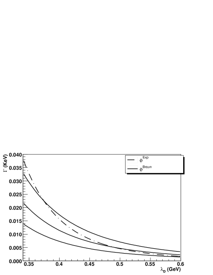
Figure 9: $\Gamma(\chi_{b0}\rightarrow PP)$ as a function $\lambda_{D}$. The dash dotted line denotes the decay rate calculated with $\phi^{\textrm{Exp}}$, while the three solid lines with $\phi^{\textrm{Braun}}$. For $\phi^{\textrm{Braun}}$ we vary the value of the parameter $\sigma_{D}$ from $\sigma_{D}=1$ (lower curve) to $\sigma_{D}=1.4$ (middle curve) to $\sigma_{D}=1.8$ (upper curve).

Figs. 8 - 9 also describe the relation between the decay rate $\Gamma(\chi_{b0}\rightarrow V_{L}V_{L})$ and $\lambda_{D^{*}_{L}}$. According to Eqs. (46) and (47), the processes $\chi_{b2}\rightarrow PP$, $\chi_{b2}\rightarrow V_{L}V_{L}$, and $\chi_{b2}\rightarrow V_{T}V_{T}$ show an analogous dependence on the first inverse moments of the light-cone distribution amplitudes, and they differ from Figs. 8 - 9 by constant pre-factors. Therefore, we do not show explicitly their plots.

Qualitatively, Figs. 8 - 9 show a dramatic dependence of the decay rate on the inverse moment $\lambda_{D}$. Using Eqs. (45), (60) and (80), one can show that when $\phi^{\rm{Braun}}$ is used, the decay rate is proportional to $\lambda_{D}^{-4}$, while it scales as $\lambda_{D}^{-6-4g}$ when we adopt $\phi^{\rm{Exp}}$, with $g$ defined in Eq. (69). As a consequence, the decay rate drops by an order of magnitude when $\lambda_{D}$ goes from $0.350$ GeV to $0.600$ GeV. The particular sensitivity of exclusive bottomonium decays into two charmed mesons to the light-cone structure of the $D$ meson —much stronger than usually observed in $D$- and $B$-decay observables— is due to the dependence of the amplitude on the product of two distributions (one for each meson) and to the non-trivial dependence of the matching coefficient $T$ on the light-quark momentum labels $\omega$ and $\bar{\omega}$ at tree level. On one hand, the strong dependence on a relatively poorly known quantity prevents us from predicting the decay rate $\Gamma(\chi_{b0}\rightarrow DD)$. On the other hand, however, it suggests that, if the decay rate is measured, this channel could be used to better determine interesting properties of the $D$-meson distribution amplitude, such as $\lambda_{D}$ and $\sigma_{D}$. The viability of this suggestion relies on the control over the theoretical error attached to the curves in Fig. 8 and on the actual chances to observe the process $\chi_{b}\rightarrow DD$ at current experiments.

The uncertainty of the decay rate stems mainly from three sources. First, there are corrections coming from subleading EFT operators. In matching $\text{NRQCD}+\text{SCET}$ onto $\text{pNRQCD}+\text{bHQET}$ (Sec. IV.1), we neglected the subleading $\text{EFT}_{\text{II}}$ operators that are suppressed by powers of $\Lambda_{\rm{QCD}}/m_{c}$ and $w^{2}$, relative to the leading $\text{EFT}_{\text{II}}$ operators in Eqs. (31) and (32). In matching QCD onto $\text{NRQCD}+\text{SCET}$ (Sec. III.1), we kept only $J_{\text{EFT}_{\text{I}}}$ (6) and neglected subleading $\text{EFT}_{\text{I}}$ operators, suppressed by powers of $\lambda$ and $w^{2}$. These subleading $\text{EFT}_{\text{I}}$ operators would match onto subleading $\text{EFT}_{\text{II}}$ operators, suppressed by powers of $\Lambda_{\rm{QCD}}/m_{c}$ and $w^{2}$. Using $w^{2}\sim 0.1$ and $\Lambda_{\rm{QCD}}/m_{c}\sim 0.3$, we find a conservative estimate for the non-perturbative corrections to be about $30\%$.

Second, there are perturbative corrections to the matching coefficients $C$ and $T$. Since $\alpha_{s}(2m_{b})=0.178$, we expect a $20\%$ correction from the one-loop contributions in matching QCD onto $\text{NRQCD}+\text{SCET}$. In the second matching step, similarly, the one-loop corrections to $T(\omega,\bar{\omega},\mu,\mu^{\prime};\,^{2S+1}L_{J})$ would be proportional to $\alpha_{s}(m_{c})\sim 30\%$. We can get an idea of their relevance by estimating the dependence of the decay rate (45) on the matching scales $\mu_{b}$ and $\mu^{\prime}_{c}$. If the matching coefficients $C$ and $T$ and the anomalous dimensions $\gamma_{\text{EFT}_{\text{I}}}$ and $\gamma_{\mathcal{O}}(\omega,\omega^{\prime},\bar{\omega},\bar{\omega}^{\prime};\mu^{\prime})$ were known at all orders, the decay rate would be independent of the matching scales $\mu_{b}$ and $\mu^{\prime}_{c}$. However, since we only know the first terms in the perturbative expansions, the decay rate bears a residual renormalization-scale dependence, whose size is determined by the first neglected terms.

In Fig. 10 we show the effect of varying $\mu_{b}$ between $4m_{b}\sim 20$ GeV and $m_{b}\sim 5$ GeV on the decay rate, using $\phi^{\rm{Braun}}$. The solid line represents the choice $\mu_{b}=2m_{b}$, while the dashed and dotted lines, which overlap almost perfectly, correspond respectively to $\mu_{b}=20$ GeV and $\mu_{b}=5$ GeV. The dependence on $\mu_{b}$ is mild, its effect being a variation of about $5\%$. We obtain analogous results for the decay rate computed with $\phi^{\rm{Exp}}$, which are not shown here in order to avoid redundancy.

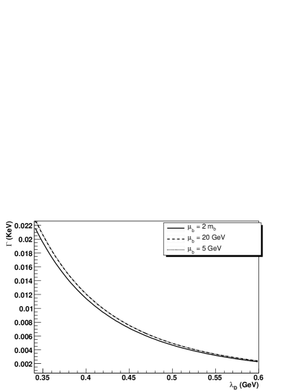
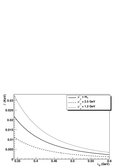
Figure 10: Left: Scale dependence of $\Gamma(\chi_{b0}\rightarrow PP)$ on the matching scale $\mu_{b}$. We vary $\mu_{b}$ from a central value $\mu_{b}=2m_{b}$ (solid line) to a maximum of $\mu_{b}=20$ GeV (dashed line) and a minimum of $\mu_{b}=5$ GeV (dotted line). The dashed and dotted lines overlap almost perfectly. Right: Scale dependence of $\Gamma(\chi_{b0}\rightarrow PP)$ on the matching scale $\mu^{\prime}_{c}$. We varied $\mu^{\prime}_{c}$ from a central value of $\mu^{\prime}_{c}=m_{c}$ (solid line) to a maximum of $\mu^{\prime}_{c}=2.5$ GeV (dashed line) and a minimum of $\mu^{\prime}_{c}=1.2$ GeV (dotted line).

On the other hand, even after the resummation, the decay rate strongly depends on $\mu^{\prime}_{c}$. We vary this scale between $1.2$ GeV and $2.5$ GeV and we observe an overall variation of about $50\%$. We expect the scale dependence to be compensated by the one-loop corrections to the matching coefficient $T(\omega,\bar{\omega},\mu,\mu^{\prime};\,^{3}P_{J})$. This observation is reinforced by the fact that the numerical values of the running factors $U(\mu_{b},\mu)$ and $V(\mu^{\prime}_{c},\mu^{\prime})$ (defined respectively in Eqs. (26) and (70)) at NLL accuracy are smaller than expected on the basis of naive counting of the logarithms. As a consequence, the next-to-leading-order corrections to the matching coefficient could be as large as the effect of the NLL resummation. In the light of Fig. 10, the one-loop correction to $T(\omega,\bar{\omega},\mu,\mu^{\prime};\,^{3}P_{J})$ seems to be an important ingredient for a reliable estimate of the decay rate.

A third source of error comes from the unknown functional form of the $D$-meson distribution amplitude. For the study of the $B$-meson shape function, an expansion in a complete set of orthonormal functions has recently been proposed and it has provided a systematic procedure to control the uncertainties due to the unknown functional form Ligeti:2008ac . The same method should be generalized to the $B$- and $D$-meson distribution amplitudes, in order to reduce the model dependence of the decay rate. We leave such an analysis to future work.

To summarize, the calculation of the one-loop matching coefficients and the inclusion of power corrections of order $\Lambda_{\rm{QCD}}/m_{c}$ appear to be necessary to provide a decay rate with an accuracy of $10\%$, that would make the decays $\chi_{bJ}\rightarrow D^{+}D^{-}$, $\chi_{bJ}\rightarrow D^{0}\bar{D}^{0}$ competitive processes to improve the determination of $\lambda_{D}$ and $\sigma_{D}$, if the experimental decay rate is observed with comparable accuracy.

We estimate the decay rate $\Gamma(\eta_{b}\rightarrow PV_{L}+\rm{c.c.})$ (48) using $\phi^{\textrm{Exp}}$ and $\phi^{\textrm{Braun}}$ for both $\phi_{P}$ and $\phi_{V_{L}}$. In the limit $m_{c}\to\infty$, spin symmetry of the bHQET Lagrangian would imply the equality of the pseudoscalar and vector distribution amplitudes, $\phi_{P}=\phi_{V_{L}}$, and hence the vanishing of the decay rate $\Gamma(\eta_{b}\rightarrow PV_{L}+\rm{c.c.})$. Assuming spin-symmetry violations, the decay rate depends on (i) the two parameters $\bar{\lambda}_{D}=(\lambda_{D}+\lambda_{D^{*}_{L}})/2$ and $\delta=(\lambda_{D^{*}_{L}}-\lambda_{D})/(\lambda_{D}+\lambda_{D^{*}_{L}})$, if $\phi^{\textrm{Exp}}$ is used, and on (ii) three parameters $\bar{\lambda}_{D}$, $\delta$, and $|\sigma_{D^{*}_{L}}-\sigma_{D}|$, if $\phi^{\textrm{Braun}}$ is used.

The two plots in the left column of Fig. 11 show the decay rate, computed with $\phi^{\rm{Exp}}$, as a function of $\bar{\lambda}_{D}$ with $\delta$ adopting various values, and as a function of $\delta$ with $\bar{\lambda}_{D}$ now being the parameter. In the right column, the decay rate computed with $\phi^{\rm{Braun}}$ is shown. Since in this case the decay rate does not strongly depend on $\delta$, we fix it at $\delta=0$ and we show the dependence of the decay rate on $\bar{\lambda}_{D}$ and $|\sigma_{D^{*}_{L}}-\sigma_{D}|$. We “normalize” the difference between the first logarithmic moments by dividing them by $\sigma=2\sigma_{D}$.

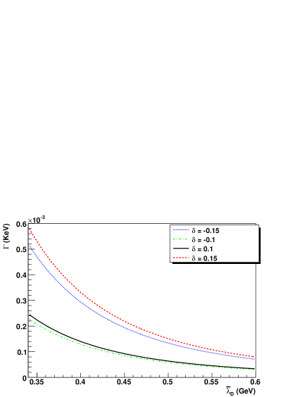
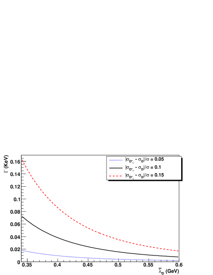
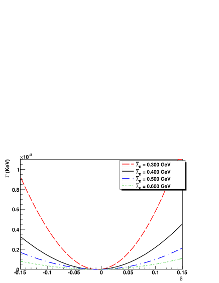
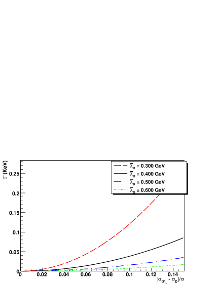
Figure 11: Left: $\Gamma(\eta_{b}\rightarrow PV_{L}+\rm{c.c.})$ as a function of $\lambda_{D}$ and $\delta$, computed using exponential distribution amplitudes $\phi^{\rm{Exp}}_{P}$ and $\phi^{\rm{Exp}}_{V_{L}}$. Right: $\Gamma(\eta_{b}\rightarrow PV_{L}+\rm{c.c.})$ as a function of $\lambda_{D}$ and $|\sigma_{D^{*}_{L}}-\sigma_{D}|/\sigma$, computed with the Braun distribution amplitudes $\phi^{\rm{Braun}}_{P}$ and $\phi^{\rm{Braun}}_{V_{L}}$.

The most striking feature of Fig. 11 is the huge sensitivity to the chosen functional form. Though a precise comparison is difficult, due to the dependence on different parameters, the decay rate increases by two orders of magnitude when we switch from $\phi^{\rm{Exp}}$ to $\phi^{\rm{Braun}}$. Once again, this effect hinders our ability to predict $\Gamma(\eta_{b}\rightarrow PV_{L}+\rm{c.c.})$ but it opens up the interesting possibility to discriminate between different model distribution amplitudes.

Using Eqs. (48) and (81), we know that $\Gamma(\eta_{b}\rightarrow PV_{L}+\rm{c.c.})$ goes like $\bar{\lambda}_{D}^{-4-4g}$ when $\phi^{\textrm{Exp}}$ used or $\bar{\lambda}_{D}^{-4}$ when $\phi^{\textrm{Braun}}$ used. Fig. 11 appears to confirm this strong dependence on $\bar{\lambda}_{D}$. The plots in the lower half of Fig. 11 reflect the fact that the decay rate vanishes if one assumes $\phi_{P}(\omega)=\phi_{V_{L}}(\omega)$.

We conclude this section with the determination of the branching ratios $\mathcal{B}(\chi_{b0}\rightarrow PP)=\Gamma(\chi_{b0}\rightarrow PP)/\Gamma(\chi_{b0}\rightarrow\textrm{light hadrons})$ and $\mathcal{B}(\eta_{b}\rightarrow PV_{L}+\textrm{c.c.})=\Gamma(\eta_{b}\rightarrow PV_{L}+\textrm{c.c.})/\Gamma(\eta_{b}\rightarrow\textrm{light hadrons})$. At leading order in pNRQCD, the only non-perturbative parameter involved in the inclusive decay width of the $\eta_{b}$ is $|R_{\eta_{b}}(0)|^{2}$ Bodwin:1994jh ,

$$\Gamma(\eta_{b}\rightarrow\text{light hadrons})=\frac{2\textrm{Im}f_{1}(^{1}S_{0})}{m^{2}_{b}}\frac{N_{c}}{2\pi}|R_{\eta_{b}}(0)|^{2}\;.$$ (62)

Therefore, $\mathcal{B}(\eta_{b}\rightarrow PV_{L}+\rm{c.c.})$ does not depend on the quarkonium wavefunction and the only non-perturbative parameters in $\mathcal{B}(\eta_{b}\rightarrow PV_{L}+\rm{c.c.})$ are those describing the $D$-meson distribution amplitudes.

For $P$-wave states, the inclusive decay rate was obtained in Refs. Bodwin:1994jh Bodwin:1992ye , where the contributions of the configurations in which the quark-antiquark pair is in a color-octet $S$-wave state were first recognized. In pNRQCD the inclusive decay rate is written as Brambilla:2001xy Brambilla:2002nu

$$\Gamma(\chi_{b0}\rightarrow\text{light hadrons})=\frac{1}{m_{b}^{4}}\frac{3N_{c}}{\pi}|R^{\prime}_{\chi_{b}}(0)|^{2}\left[\textrm{Im}f_{1}(^{3}P_{0})+\frac{1}{9N_{c}^{2}}\textrm{Im}f_{8}(^{3}S_{1})\mathcal{E}\right]\;,$$ (63)

where the color-octet matrix element has been expressed in terms of the heavy quarkonium wavefunction and of the gluonic correlator $\mathcal{E}$, whose precise definition is given in Ref. Brambilla:2001xy . $\mathcal{E}$ is a universal parameter and is completely independent of any particular heavy quarkonium state under consideration. Its value has been obtained by fitting to existing charmonium data and, thanks to the universality, the same value can be used to predict properties of bottomonium decays. It is found in Ref. Brambilla:2001xy $\mathcal{E}=5.3\,^{+3.5}_{-2.2}$. The matching coefficients in Eqs. (62) and (63) are known to one loop. For the updated value we refer to Ref. Vairo:2003gh and references therein. For reference, the tree-level values of the coefficients are as follows Bodwin:1994jh :

$$\textrm{Im}f_{1}(^{1}S_{0})=\alpha^{2}_{s}(2m_{b})\pi\frac{C_{F}}{2N_{c}}\;,\quad\textrm{Im}f_{1}(^{3}P_{0})=3\alpha^{2}_{s}(2m_{b})\pi\frac{C_{F}}{2N_{c}}\;,\quad\textrm{Im}f_{8}(^{3}S_{1})=\frac{n_{f}}{6}\alpha^{2}_{s}(2m_{b})\pi\;.$$ (64)

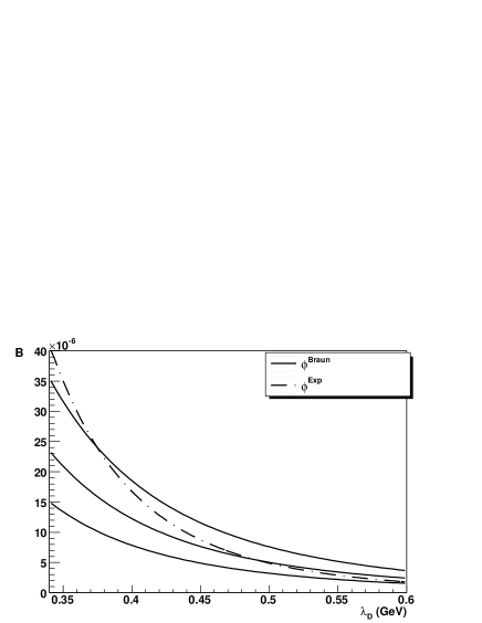
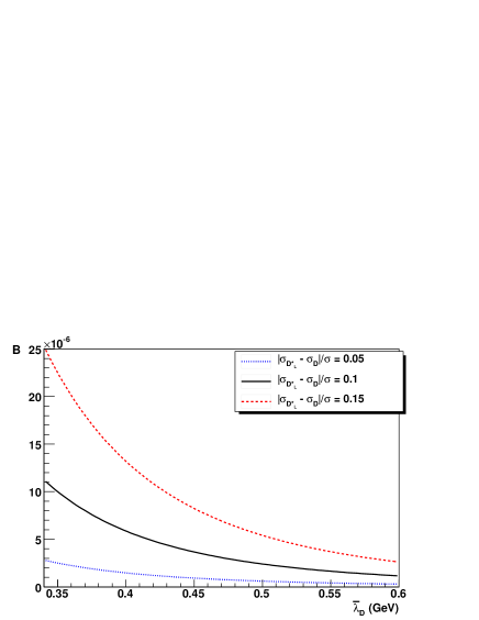
Figure 12: Branching ratios $\mathcal{B}(\chi_{b0}\rightarrow PP)$ (left) and $\mathcal{B}(\eta_{b}\rightarrow PV_{L}+\rm{c.c.})$ (right). The latter is computed using the distribution amplitude $\phi^{\rm{Braun}}$.

With the above parameters, we plot $\mathcal{B}(\chi_{b0}\rightarrow PP)$ and $\mathcal{B}(\eta_{b}\rightarrow PV_{L}+\rm{c.c.})$ as a function of $\lambda_{D}$ and $\bar{\lambda}_{D}$, respectively, in Fig. 12. Over the range of $\lambda_{D}$ we are considering, $\mathcal{B}(\chi_{b0}\rightarrow PP)$ varies between $4\cdot 10^{-5}$ and $4\cdot 10^{-6}$; it is approximately one or two orders of magnitude smaller than the branching ratios observed in Ref. :2008sx for $\chi_{bJ}$ decays into light hadrons. $\mathcal{B}(\eta_{b}\rightarrow PV_{L}+\rm{c.c.})$ depends on the choice of the distribution amplitude. Choosing the parameterization $\phi^{\rm{Braun}}$ (59), it appears that, despite the suppression at $|\sigma_{D^{*}_{L}}-\sigma_{D}|=0$, $\mathcal{B}(\eta_{b}\rightarrow PV_{L}+\rm{c.c.})$ assumes values comparable to $\mathcal{B}(\chi_{b0}\rightarrow PP)$ even for a small deviation from the spin-symmetry limit. If $\phi^{\rm{Exp}}$ is chosen, the branching ratio is suppressed over a wide range of $|\sigma_{D^{*}_{L}}-\sigma_{D}|$. The branching ratio $\mathcal{B}(\eta_{b}\rightarrow PV_{L}+\rm{c.c.})$ was first estimated in Maltoni:2004hv . The authors of Maltoni:2004hv assumed that the exclusive decays into $DD^{*}$ dominate the inclusive decay into charm, $\Gamma(\eta_{b}\rightarrow PV_{L}+\textrm{c.c.})\sim\Gamma(\eta_{b}\rightarrow c\bar{c}+X)$. With this assumption, they estimated the branching ratio to be in the range $10^{-3}<\mathcal{B}(\eta_{b}\rightarrow PV_{L}+\rm{c.c.})<10^{-2}$. Our analysis shows that such an assumption does not appear to be justified in the range of $\bar{\lambda}_{D}$ considered in Fig. 12, while it would be appropriate for smaller values of the first inverse moments, for example for $\bar{\lambda}_{D}\sim 0.200$ GeV if the distribution amplitudes are described by $\phi^{\textrm{Braun}}$.

Our estimates indicate that observing the exclusive processes $\eta_{b}\rightarrow DD^{*}+\textrm{c.c.}$ and $\chi_{b}\rightarrow DD$ would be extremely challenging. A preliminary analysis for $\chi_{b}\rightarrow D^{0}\bar{D}^{0}$ italianconnection suggests that the number of $\Upsilon(2S)$ produced at BABAR allows for the measurement of a branching ratio $\mathcal{B}(\chi_{b0}\rightarrow D^{0}\bar{D}^{0})\sim 10^{-3}$, which is two or three orders of magnitude bigger than the values in Fig. 12. An even bigger branching ratio would be required for the smaller $\Upsilon(2S)$ sample of CLEO. However, we stress once again the strong dependence of the decay rates on the values of the first inverse moments. In particular, our estimates rely on the relation $\lambda_{D}=\lambda_{B}$, which is valid in the limit of $m_{b},m_{c}\rightarrow\infty$; even small corrections to the heavy flavor symmetry, if they had the effect of shifting the value of $\lambda_{D}$ towards the range $0.250-0.350$ GeV, could considerably increase the branching ratios.

VI Conclusions

In this paper we have analyzed the exclusive decays of the $C$-even bottomonia into a pair of charmed mesons. We approached the problem using a series of EFTs that lead to the factorization formulas for the decay rates (Eqs. (45) - (48)), valid at leading order in the EFT power counting and at all orders in $\alpha_{s}$. We improved the perturbative results by resumming Sudakov logarithms of the ratios of the characteristic scales that are germane to the dynamics of the processes.

The decay rates (45) - (48) receive both perturbative and non-perturbative corrections. Perturbative corrections come from loop corrections to the matching coefficients $C$ and $T$, which are respectively of order $\alpha_{s}(2m_{b})\sim 0.2$ and $\alpha_{s}(m_{c})\sim 0.3$. The largest non-perturbative contribution could be as big as $\Lambda_{\text{QCD}}/m_{c}$, which would amount approximately to a $30\%$ correction. Therefore, corrections to the leading-order decay rates could be noticeable, as the strong dependence of the decay rates on the renormalization-scale $\mu^{\prime}_{c}$ suggests. However, the EFT approach shown in this paper allows for a systematic treatment of both perturbative corrections and power-suppressed operators, so that, if the experimental data require, it is possible to extend the present analysis beyond the leading order.

For simplicity, we have focused in this paper on the decays of $C$-even bottomonia, in which cases the decays proceed via two intermediate gluons and both the matching coefficients $C$ and $T$ are non-trivial at tree level. The same EFT approach can be applied to the decays of $C$-odd states, in particular, to the decays $\Upsilon\rightarrow DD$ and $\Upsilon\rightarrow D^{*}D^{*}$, with the complication that the matching coefficient $T$ arises only at one-loop level. Moreover, the same EFT formalism developed in this paper can be applied to the study of the channels that have vanishing decay rates at leading order in the power counting, such as $\eta_{b}\rightarrow D^{*}D^{*}$, $\Upsilon\rightarrow DD^{*}+\textrm{c.c.}$, and $\chi_{b2}\rightarrow DD^{*}+\textrm{c.c.}$. Experimental data for the charmonium system show that, for the decays of charmonium into light hadrons, the expected suppression of the subleading twist processes is not seen. It is interesting to see whether such an effect appears in bottomonium decays into two charmed mesons, using the EFT approach of this paper to evaluate the power-suppressed decay rates.

Finally, in Sec. V we used model distribution amplitudes to estimate the decay rates. The most evident, qualitative feature of the decay rates is the strong dependence on the parameters of the $D$-meson distribution amplitude. Even though this feature may prevent us from giving reliable estimates of the decay rates or of the branching ratios, it makes the channels analyzed here ideal candidates for the extraction of important $D$-meson parameters, when the branching ratios can be observed with sufficient accuracy.

Appendix A Solution of the running equation in pNRQCD + bHQET

The RGE in Eq. (57) can be solved by applying the methods discussed in Ref. Lange:2003ff to find the evolution of the $B$-meson distribution amplitude. We generalize this approach to the specific case discussed here, where two distribution amplitudes are present. Following Ref. Lange:2003ff , we define

$$\omega\Gamma(\omega,\omega^{\prime},\alpha_{s})=-\frac{\alpha_{s}C_{F}}{\pi}\left[\theta\left({\omega}-{\omega}^{\prime}\right)\left(\frac{1}{{\omega}-{\omega}^{\,\prime}}\right)_{+}+\theta\left({\omega}^{\prime}-{\omega}\right)\theta\left({\omega}\right)\frac{{\omega}}{{\omega}^{\prime}}\left(\frac{1}{{\omega}^{\prime}-{\omega}}\right)_{+}\right]\;.$$

Lange and Neubert Lange:2003ff prove that

$$\int d\omega^{\prime}\omega\Gamma(\omega,\omega^{\prime},\alpha_{s})(\omega^{\prime})^{a}=\omega^{a}\mathcal{F}(a,\alpha_{s})\;,$$ (65)

with

$$\mathcal{F}(a,\alpha_{s})=\frac{\alpha_{s}C_{F}}{\pi}\left[\psi(1+a)+\psi(1-a)+2\gamma_{E}\right]\;.$$

$\psi$ is the digamma function and $\gamma_{E}$ the Euler constant. Eq. (65) is valid if $-1<\textrm{Re}\,a<1$. Exploiting (65), a solution of the running equation Eq. (57) with initial condition $T(\omega,\bar{\omega},\mu_{0}^{\prime})=\left(\omega/\mu_{0}^{\prime}\right)^{\eta}\left(\bar{\omega}/\mu_{0}^{\prime}\right)^{\xi}$ at a certain scale $\mu_{0}^{\prime}$ is

$$F^{2}(\mu^{\prime})T(\omega,\bar{\omega},\mu^{\prime})=F^{2}(\mu^{\prime}_{0})f(\omega,\mu^{\prime},\mu_{0}^{\prime},\eta)f(\bar{\omega},\mu^{\prime},\mu_{0}^{\prime},\xi)\;,$$ (66)

with

$$\begin{split}&f(\omega,\mu^{\prime},\mu_{0}^{\prime},\eta)=\left(\frac{\omega}{\mu_{0}^{\prime}}\right)^{\eta-g}\left(\bar{n}\cdot v\right)^{g}\exp U(\mu_{0}^{\prime},\mu^{\prime},\eta)\;,\\ &g\equiv g(\mu_{0}^{\prime},\mu^{\prime})=\int_{\alpha_{s}(\mu_{0}^{\prime})}^{\alpha_{s}(\mu^{\prime})}\frac{d\alpha}{\beta(\alpha)}\Gamma_{\textrm{cusp}}(\alpha)\;,\\ &U(\mu_{0}^{\prime},\mu^{\prime},\eta)=\int_{\alpha_{s}(\mu_{0}^{\prime})}^{\alpha_{s}(\mu^{\prime})}\frac{d\alpha}{\beta(\alpha)}\left[\Gamma_{\textrm{cusp}}(\alpha)\int_{\alpha_{s}(\mu_{0}^{\prime})}^{\alpha}\frac{d\alpha^{\prime}}{\beta(\alpha^{\prime})}+\gamma_{1}(\alpha)+\mathcal{F}(\eta-g,\alpha)\right]\;,\\ &\gamma_{1}(\alpha_{s})=-2\frac{\alpha_{s}C_{F}}{4\pi}\;.\end{split}$$ (67)

The function $f(\bar{\omega},\mu^{\prime},\mu_{0}^{\prime},\xi)$ has the same form as $f(\omega,\mu^{\prime},\mu_{0}^{\prime},\eta)$ and is obtained by replacing $\omega\rightarrow\bar{\omega}$, $\eta\rightarrow\xi$, and $\bar{n}\cdot v\rightarrow n\cdot v^{\prime}$ in Eq. (67). The integrals over $\alpha$ can be performed explicitly using the beta function in Eq. (28). The result is

$$\begin{split}f(\omega,\mu^{\prime},\mu_{0}^{\prime},\eta)f(\bar{\omega},\mu^{\prime},\mu_{0}^{\prime},\xi)=&\left(\frac{\omega}{\mu_{0}^{\prime}}\right)^{\eta-g}\left(\frac{\bar{\omega}}{\mu_{0}^{\prime}}\right)^{\xi-g}\left(\bar{n}\cdot v\,n\cdot v^{\prime}\right)^{g}\exp\left[V(\mu_{0}^{\prime},\mu^{\prime})\right]\\ &\frac{\Gamma(1-\eta+g)\Gamma(1+\eta)}{\Gamma(1+\eta-g)\Gamma(1-\eta)}\frac{\Gamma(1-\xi+g)\Gamma(1+\xi)}{\Gamma(1+\xi-g)\Gamma(1-\xi)}\;,\end{split}$$ (68)

Where, at NLL,

$$g(\mu_{0}^{\prime},\mu^{\prime})=-\frac{\Gamma^{(0)}_{\rm{cusp}}}{2\beta_{0}}\left\{\ln r+\left(\frac{\Gamma^{(1)}_{\rm{cusp}}}{\Gamma_{\rm{cusp}}^{(0)}}-\frac{\beta_{1}}{\beta_{0}}\right)\frac{\alpha_{\rm{s}}(\mu_{0}^{\prime})}{4\pi}(r-1)\right\}\;,$$ (69)

and

$$\begin{split}V(\mu_{0}^{\prime},\mu^{\prime})=&-\Gamma^{(0)}_{\textrm{cusp}}\frac{2\pi}{\beta_{0}^{2}}\left\{\frac{r-1-r\ln r}{\alpha_{s}(\mu^{\prime})}+\left(\frac{\Gamma^{(1)}_{\textrm{cusp}}}{\Gamma^{(0)}_{\textrm{cusp}}}-\frac{\beta_{1}}{\beta_{0}}\right)\frac{1-r+\ln r}{4\pi}+\frac{\beta_{1}}{8\pi\beta_{0}}\ln^{2}r\right\}\\ &+\frac{C_{F}}{\beta_{0}}\left(2-8\gamma_{E}\right)\ln r\;,\end{split}$$ (70)

with $r=\alpha_{s}(\mu^{\prime})/\alpha_{s}(\mu_{0}^{\prime})$. Notice that in the running from $\mu_{0}^{\prime}=m_{c}$ to $\mu^{\prime}=1$ GeV only three flavors are active, so in the expressions for $\beta_{0}$, $\beta_{1}$, and $\Gamma^{(1)}_{\textrm{cusp}}$ we use $n_{f}=3$.

Eq. (68) is the solution for the initial condition $T(\omega,\bar{\omega},\mu_{0}^{\prime})=\left(\omega/\mu_{0}^{\prime}\right)^{\eta}\left(\bar{\omega}/\mu_{0}^{\prime}\right)^{\xi}$. To solve the RGE for a generic initial condition, we express $T$ as the Fourier transform with respect to $\ln\omega/\mu_{0}^{\prime}$,

$$\begin{split}T(\omega,\bar{\omega},\mu_{0}^{\prime})&=\frac{1}{(2\pi)^{2}}\int_{-\infty}^{+\infty}drds\exp\left(-ir\ln\frac{\omega}{\mu_{0}^{\prime}}\right)\exp\left(-is\ln\frac{\bar{\omega}}{\mu_{0}^{\prime}}\right)F[T](r,s,\mu_{0}^{\prime})\\ &=\frac{1}{(2\pi)^{2}}\int_{-\infty}^{+\infty}drds\left(\frac{\omega}{\mu_{0}^{\prime}}\right)^{-ir}\left(\frac{\bar{\omega}}{\mu_{0}^{\prime}}\right)^{-is}F[T](r,s,\mu_{0}^{\prime})\;,\end{split}$$

where $F[T]$ denotes the Fourier transform of $T$. From the solution (66)-(68) it follows that

$$\begin{split}F^{2}(\mu^{\prime})T(\omega,\bar{\omega},\mu^{\prime})=&\frac{F^{2}(\mu^{\prime}_{0})}{(2\pi)^{2}}\int_{-\infty}^{+\infty}drds\left(\frac{\omega}{\mu_{0}^{\prime}}\right)^{-ir-g}\left(\frac{\bar{\omega}}{\mu_{0}^{\prime}}\right)^{-is-g}\left(\bar{n}\cdot v\,n\cdot v^{\prime}\right)^{g}F[T](r,s,\mu_{0}^{\prime})\\ &\exp\left[V(\mu_{0}^{\prime},\mu^{\prime})\right]\frac{\Gamma(1+ir+g)\Gamma(1-ir)}{\Gamma(1-ir-g)\Gamma(1+ir)}\frac{\Gamma(1+is+g)\Gamma(1-is)}{\Gamma(1-is-g)\Gamma(1+is)}\;.\end{split}$$ (71)

The Fourier transform of the matching coefficient in Eq. (71) has to be understood in the sense of distributions Distribution . That is, we define the Fourier transform of $T$ as the function of $r$ and $s$ that satisfies

$$\frac{1}{(2\pi)^{2}}\int drds\,F[T](r,s,\mu^{\prime})\varphi_{A}(r,\mu^{\prime})\varphi_{B}(s,\mu^{\prime})=\int_{0}^{+\infty}\frac{d\omega}{\omega}\frac{d\bar{\omega}}{\bar{\omega}}T(\omega,\bar{\omega},\mu^{\prime})\phi_{A}(\omega,\mu^{\prime})\phi_{B}(\bar{\omega},\mu^{\prime})\;,$$ (72)

or, more precisely, $F[T](r,s,\mu^{\prime})$ is the linear functional that acts on the test functions $\varphi_{A}(r)$ and $\varphi_{B}(s)$ according to

$$\frac{1}{(2\pi)^{2}}(F[T](r,s,\mu^{\prime}),\,\varphi_{A}(r,\mu^{\prime})\varphi_{B}(s,\mu^{\prime}))=\int_{0}^{+\infty}\frac{d\omega}{\omega}\frac{d\bar{\omega}}{\bar{\omega}}T(\omega,\bar{\omega},\mu^{\prime})\phi_{A}(\omega,\mu^{\prime})\phi_{B}(\bar{\omega},\mu^{\prime})\;.$$ (73)

The function $\varphi_{A}$ is the Fourier transform of the $D$-meson distribution amplitude,

$$\varphi_{A}(r,\mu^{\prime})=\int_{0}^{\infty}\frac{d\omega}{\omega}\left(\frac{\omega}{\mu^{\prime}}\right)^{ir}\phi_{A}(\omega,\mu^{\prime})\;,$$ (74)

where the integral on the r.h.s. should converge in the ordinary sense because of the regularity properties of the $D$-meson distribution amplitude. As in Sec. IV, the subscript $A$ denotes the spin and polarization of the $D$ meson.

In the distribution sense, the Fourier transform of the coefficient $1/(\omega+\bar{\omega})$ is

$$\begin{split}F\left[\frac{1}{\omega+\bar{\omega}}\right](r,s,\mu_{0}^{\prime})&=(2\pi)^{2}\frac{1}{2\mu_{0}^{\prime}}\delta(r+s+i)\,\textrm{sech}\left[\frac{\pi}{2}(r-s)\right]\\ &=\frac{1}{2}(2\pi)^{2}\frac{1}{2\mu_{0}^{\prime}}\delta(R+i)\,\textrm{sech}\left[\frac{\pi}{2}S\right]\;,\end{split}$$ (75)

where $R=r+s$, $S=r-s$, and the factor $\frac{1}{2}$ comes from the Jacobian of the change of variables. The hyperbolic secant is defined as $\rm{sech}=1/\cosh$. Similarly, we find

$$\begin{split}F\left[\frac{\omega-\bar{\omega}}{\omega+\bar{\omega}}\right](R,S,\mu_{0}^{\prime})=\frac{i}{2}(2\pi)^{2}\delta(R)\,\left(\textrm{cosech}\left[\frac{\pi}{2}S+i\varepsilon\right]+\textrm{cosech}\left[\frac{\pi}{2}S-i\varepsilon\right]\right)\;.\end{split}$$ (76)

The $\delta$ function in Eq. (75) has complex argument. The definition is analogous to the one in real space Distribution ,

$$(\delta(R+i),\varphi(R))=\varphi(-i)\;.$$ (77)

Using Eqs. (75) and (76), we can perform the integral in Eq. (71), obtaining respectively $T(\omega,\bar{\omega},\mu,\mu^{\prime};\,^{3}P_{J})$ and $T(\omega,\bar{\omega},\mu,\mu^{\prime};\,^{1}S_{0})$. In order to give an explicit example, we proceed using Eq. (75). Integrating the $\delta$ function we are left with

$$\begin{split}&F^{2}(\mu^{\prime})T(\omega,\bar{\omega};\mu^{\prime})=F^{2}(\mu_{0}^{\prime})\exp\left[V(\mu_{0}^{\prime},\mu^{\prime})\right]\frac{1}{\mu_{0}^{\prime}}\left(\frac{\mu_{0}^{\prime\,2}}{\omega\bar{\omega}}\right)^{1/2+g}\left(\bar{n}\cdot v\,n\cdot v^{\prime}\right)^{g}\\ &\int_{-\infty}^{\infty}dS\exp\left[-i\frac{S}{2}\ln\frac{\omega}{\bar{\omega}}\right]\textrm{sech}\left[\frac{\pi}{2}S\right]\frac{1}{1+S^{2}}\frac{\Gamma\left(\frac{3}{2}+g+\frac{i}{2}S\right)}{\Gamma\left(\frac{1}{2}-g-\frac{i}{2}S\right)}\frac{\Gamma\left(\frac{3}{2}+g-\frac{i}{2}S\right)}{\Gamma\left(\frac{1}{2}-g+\frac{i}{2}S\right)}\;.\end{split}$$ (78)

The integral (78) can be done by contour. The integrand has poles along the imaginary axis. In $S=\pm i$ there is a double pole, coming from the coincidence of one pole of the hyperbolic secant and the singularities in $1/(1+S^{2})$. The $\Gamma$ functions in the numerator have poles respectively in $S=\pm i\left(2n+3+2g\right)$ with $n>0$, while the other poles of sech are in $S=\pm i(2n+1)$, with $n\geq 1$. We close the contour in the upper half plane for $\bar{\omega}>\omega$ and in the lower half plan for $\omega>\bar{\omega}$, obtaining

$$\begin{split}&F^{2}(\mu^{\prime})T(\omega,\bar{\omega},\mu^{\prime})=F^{2}(\mu_{0}^{\prime})\exp\left[V(\mu^{\prime}_{0},\mu^{\prime})\right]\,\theta(\bar{\omega}-\omega)\frac{1}{\bar{\omega}}\left(\frac{\mu_{0}^{\prime\,2}\bar{n}\cdot v\,n\cdot v^{\prime}}{\omega\bar{\omega}}\right)^{g}\\ &\qquad\left\{\frac{\Gamma(1+g)\Gamma(2+g)}{\Gamma(1-g)\Gamma(-g)}\left[1-\ln\frac{\omega}{\bar{\omega}}+\psi(1-g)-\psi(-g)+\psi(1+g)-\psi(2+g)\right]\right.\\ &\left.+\sum_{n=1}^{\infty}(-)^{n+1}\left(\frac{\omega}{\bar{\omega}}\right)^{n}\frac{1}{n(n+1)}\frac{\Gamma(1-n+g)\Gamma(2+n+g)}{\Gamma(-n-g)\Gamma(1-g+n)}\right.\\ &\left.-\sum_{n=1}^{\infty}\left(\frac{\omega}{\bar{\omega}}\right)^{n+g}\frac{\pi}{(n-1)!}\textrm{csc}(g\pi)\frac{1}{(n+g)(1+n+g)}\frac{\Gamma(2+n+2g)}{\Gamma(1+n)\Gamma(-n-2g)}\right\}+\left(\omega\rightarrow\bar{\omega}\right)\;,\end{split}$$ (79)

with csc$(g\pi)=1/\sin(g\pi)$ and $\psi$ is the digamma function. More compactly, we can express Eq. (79) using the hypergeometric functions ${}_{4}F_{3}$ and ${}_{3}F_{2}$,

$$\begin{split}&F^{2}(\mu^{\prime})\,T(\omega,\bar{\omega},\mu,\mu^{\prime};\,^{3}P_{J})=F^{2}(\mu^{\prime}_{c})\frac{C_{F}}{N_{c}^{2}}\frac{4\pi\alpha_{s}(\mu^{\prime}_{c})}{m_{b}}\exp\left[V(\mu^{\prime}_{c},\mu^{\prime})\right]\,\left(\frac{\mu^{\prime\,2}_{c}\bar{n}\cdot vn\cdot v^{\prime}}{\omega\,\bar{\omega}}\right)^{g}\\ &\frac{\theta(\bar{\omega}-\omega)}{\bar{\omega}}\left\{\frac{\Gamma(1+g)\Gamma(2+g)}{\Gamma(1-g)\Gamma(-g)}\left[1-\ln\frac{\omega}{\bar{\omega}}+\psi(1-g)-\psi(-g)+\psi(1+g)-\psi(2+g)\right]\right.\\ &\left.+\frac{1}{2}\frac{\omega}{\bar{\omega}}\,\frac{\Gamma(g+2)\Gamma(g+3)}{\Gamma(1-g)\Gamma(2-g)}\,_{4}F_{3}\left(1,1,g+2,g+3;3,1-g,2-g;-\frac{\omega}{\bar{\omega}}\right)\right.\\ &\left.-\left(\frac{\omega}{\bar{\omega}}\right)^{1+g}4\cos(g\pi)\frac{\Gamma(2+2g)^{2}}{g+2}\,_{3}F_{2}\left(g+1,2g+2,2g+3;2,g+3;-\frac{\omega}{\bar{\omega}}\right)\right\}+\left(\omega\rightarrow\bar{\omega}\right)\;,\end{split}$$ (80)

where we have introduced the constants that appear in the initial condition in Eq. (33). In the same way, we obtain

$$\begin{split}F^{2}(\mu^{\prime})\,&T(\omega,\bar{\omega},\mu,\mu^{\prime};\,^{1}S_{0})=F^{2}(\mu^{\prime}_{c})\frac{C_{F}}{2N_{c}^{2}}\frac{4\pi\alpha_{s}(\mu^{\prime}_{c})}{m_{b}}\exp\left[V(\mu^{\prime}_{c},\mu^{\prime})\right]\,\theta(\bar{\omega}-\omega)\left(\frac{\mu^{\prime\,2}_{c}\bar{n}\cdot vn\cdot v^{\prime}}{\omega\,\bar{\omega}}\right)^{g}\\ &\left\{2\frac{\Gamma(1+g)\Gamma(2+g)}{\Gamma(1-g)\Gamma(2-g)}\frac{\omega}{\bar{\omega}}\,_{3}F_{2}\left(1,g+1,g+2;1-g,2-g;-\frac{\omega}{\bar{\omega}}\right)+\frac{\Gamma^{2}(1+g)}{\Gamma^{2}(1-g)}\right.\\ &\left.-\left(\frac{\omega}{\bar{\omega}}\right)^{1+g}4\cos(g\pi)\Gamma(1+2g)\Gamma(2g+2)\,_{2}F_{1}\left(2g+2,2g+1;2;-\frac{\omega}{\bar{\omega}}\right)\right\}-\left(\omega\rightarrow\bar{\omega}\right)\;.\end{split}$$ (81)

In Eqs. (80) and (81) we renamed the initial scale $\mu^{\prime}_{0}=\mu^{\prime}_{c}$ to denote its connection to the scale $m_{c}$. Setting $\mu^{\prime}=\mu^{\prime}_{c}$ or, equivalently, $g=0$, it can be explicitly verified that the solutions Eqs. (80) and (81) satisfy the initial conditions Eq. (33).

Appendix B Boost transformation of the $D$-meson distribution amplitude

We derive in this Appendix the relation between the distribution amplitudes in the $D$-meson and in the bottomonium rest frames, as given in Eq. (60). In the $D$-meson rest frame, characterized by the velocity label $v_{0}=(1,0,0,0)$, the local heavy-light matrix element is defined as

$$\langle 0|\bar{\xi}^{\,\bar{l}}_{n}(0)\frac{\hbox to0.0pt{\hbox to5.00002pt{\hfil/\hfil}\hss}\bar{n}}{2}\gamma_{5}\,h^{c}_{n}(0)|D\rangle_{v_{0}}=-iF(\mu^{\prime})\frac{\bar{n}\cdot v_{0}}{2}\;.$$ (82)

The matrix element of the heavy- and light-quark fields at a light-like separation $z^{\mu}_{0}=n\cdot z_{0}\,\bar{n}^{\mu}/2$ defines the light-cone distribution $\tilde{\phi}_{0}(n\cdot z_{0},\mu^{\prime})$ in coordinate space:

$$\langle 0|\bar{\chi}^{\,\bar{l}}_{n}(n\cdot z_{0})\,\frac{\hbox to0.0pt{\hbox to5.00002pt{\hfil/\hfil}\hss}\bar{n}}{2}\gamma_{5}\,{\mathcal{H}}^{c}_{n}(0)|D\rangle_{v_{0}}=-iF(\mu^{\prime})\frac{\bar{n}\cdot v_{0}}{2}\,\tilde{\phi}_{0}(n\cdot z_{0},\mu^{\prime})\;.$$ (83)

Eqs. (82) and (83) imply $\tilde{\phi}_{0}(0,\mu^{\prime})=1$. In the definitions (82) and (83) the subscript $0$ is used to denote quantities in the $D$-meson rest frame. This convention is used in the rest of this Appendix. In the bottomonium rest frame, where the velocity label in light-cone coordinates is $v=(n\cdot v,\bar{n}\cdot v,0)$ and the light-like separation is $z^{\mu}=n\cdot z\,\bar{n}^{\mu}/2$, we define

$$\langle 0|\bar{\xi}^{\,\bar{l}}_{n}(0)\frac{\hbox to0.0pt{\hbox to5.00002pt{\hfil/\hfil}\hss}\bar{n}}{2}\gamma_{5}\,h^{c}_{n}(0)|D\rangle_{v}=-iF(\mu^{\prime})\frac{\bar{n}\cdot v}{2}$$ (84)

and

$$\langle 0|\bar{\chi}^{\,\bar{l}}_{n}(n\cdot z)\,\frac{\hbox to0.0pt{\hbox to5.00002pt{\hfil/\hfil}\hss}\bar{n}}{2}\gamma_{5}\,{\mathcal{H}}^{c}_{n}(0)|D\rangle_{v}=-iF(\mu^{\prime})\frac{\bar{n}\cdot v}{2}\,\tilde{\phi}(n\cdot z,\mu^{\prime})\;.$$ (85)

Suppose that $\Lambda$ is some standardized boost that takes the $D$ meson from $v$, its velocity in the bottomonium rest frame, to rest. It is straightforward to find the relations between the $D$-meson momenta in the two frames:

$$\begin{split}n\cdot p_{0}=\bar{n}\cdot vn\cdot p\quad\text{and}\quad\bar{n}\cdot p_{0}=n\cdot v\bar{n}\cdot p\;.\end{split}$$

There is a similar relation for the light-cone coordinates,

$$n\cdot z_{0}=\bar{n}\cdot v\,n\cdot z\;.$$

With $U(\Lambda)$, the unitary operator that implements the boost $\Lambda$, one can write

$$U(\Lambda)|D\rangle_{v}=|D\rangle_{v_{0}}\;.$$

We choose $\Lambda$ such that, for the Dirac fields,

$$U(\Lambda)\xi^{\,\bar{l}}_{n}(x)\,U^{-1}(\Lambda)=\Lambda_{{1}/{2}}^{-1}\,\xi^{\,\bar{l}}(\Lambda x)\quad\text{and}\quad U(\Lambda)h^{c}_{n}(x)\,U^{-1}(\Lambda)=\Lambda_{{1}/{2}}^{-1}\,h^{c}(\Lambda x)\;,$$

where

$$\Lambda_{{1}/{2}}=\cosh\frac{\alpha}{2}+\frac{{\hbox to0.0pt{\hbox to5.00002pt{\hfil/\hfil}\hss}\bar{n}}\hbox to0.0pt{\hbox to6.00235pt{\hfil/\hfil}\hss}n-\hbox to0.0pt{\hbox to6.00235pt{\hfil/\hfil}\hss}n{\hbox to0.0pt{\hbox to5.00002pt{\hfil$\bar{n}$\hfil}\hss}/}}{4}\sinh\frac{\alpha}{2}\;,$$

with $\alpha$ related to $v$ by $e^{\alpha}=\bar{n}\cdot v$ and $e^{-\alpha}=n\cdot v$.

Now we can write the matrix element in Eq. (84) as

$$\begin{split}\langle 0|\,\bar{\xi}^{\,\bar{l}}_{n}&\frac{\hbox to0.0pt{\hbox to5.00002pt{\hfil/\hfil}\hss}\bar{n}}{2}\gamma_{5}h^{c}_{n}(0)|D\rangle_{v}\\ &=\,\langle 0|U^{-1}(\Lambda)\left(U(\Lambda)\bar{\xi}^{\,\bar{l}}_{n}(0)U^{-1}(\Lambda)\right)\frac{\hbox to0.0pt{\hbox to5.00002pt{\hfil/\hfil}\hss}\bar{n}}{2}\gamma_{5}\left(U(\Lambda)h^{c}_{n}(0)U^{-1}(\Lambda)\right)U(\Lambda)|D\rangle_{v}\\ &=\,\langle 0|\bar{\xi}^{\,\bar{l}}(0)\Lambda_{1/2}\frac{\hbox to0.0pt{\hbox to5.00002pt{\hfil/\hfil}\hss}\bar{n}}{2}\gamma_{5}\Lambda_{1/2}^{-1}h^{c}(0)|D\rangle_{v_{0}}=\bar{n}\cdot v\,\langle 0|\bar{\xi}^{\,\bar{l}}(0)\frac{\hbox to0.0pt{\hbox to5.00002pt{\hfil/\hfil}\hss}\bar{n}}{2}\gamma_{5}h^{c}(0)|D\rangle_{v_{0}}\\ &=-iF(\mu^{\prime})\frac{\bar{n}\cdot v}{2}\bar{n}\cdot v_{0}=-iF(\mu^{\prime})\frac{\bar{n}\cdot v}{2}\;.\end{split}$$ (86)

where, in the last step, we have used $\bar{n}\cdot v_{0}=1$. Eq. (86) is thus in agreement with the definition in Eq. (84). Applying the same reasoning to Eq. (85), one finds

$$\begin{split}\langle 0|\bar{\chi}^{\,\bar{l}}_{n}(n\cdot z)\,\frac{\hbox to0.0pt{\hbox to5.00002pt{\hfil/\hfil}\hss}\bar{n}}{2}\gamma_{5}\,{\mathcal{H}}^{c}_{n}(0)|D\rangle_{v}&=\bar{n}\cdot v\,\langle 0|\bar{\chi}^{\,\bar{l}}(\bar{n}\cdot v\,n\cdot z)\,\frac{\hbox to0.0pt{\hbox to5.00002pt{\hfil/\hfil}\hss}\bar{n}}{2}\gamma_{5}\,{\mathcal{H}}^{c}(0)|D\rangle_{v_{0}}\\ &=-iF(\mu^{\prime})\frac{\bar{n}\cdot v}{2}\,\tilde{\phi}_{0}(n\cdot z_{0},\mu^{\prime})\;.\end{split}$$ (87)

Comparing Eq. (87) with (85), we see that $\tilde{\phi}(n\cdot z,\mu^{\prime})=\tilde{\phi}_{0}(\bar{n}\cdot v\,n\cdot z,\mu^{\prime})$. Note that in the bottomonium rest frame the normalization condition for the distribution amplitude is also $\tilde{\phi}(0,\mu^{\prime})=1$.

In the main text of this paper we have used the $D$-meson distribution amplitudes in momentum space,

$$\begin{split}\phi_{0}(\omega_{0},\mu^{\prime})&\equiv\frac{1}{2\pi}\int dn\cdot z_{0}\,e^{i\omega_{0}n\cdot z_{0}}\tilde{\phi}_{0}(n\cdot z_{0},\mu^{\prime})\;,\\ \phi(\omega,\mu^{\prime})&\equiv\frac{1}{2\pi}\int dn\cdot z\,e^{i\omega n\cdot z}\tilde{\phi}(n\cdot z,\mu^{\prime})\;.\end{split}$$

Using Eq. (87), we can relate the two distributions:

$$\begin{split}\phi(\omega,\mu^{\prime})&=\frac{1}{2\pi}\int dn\cdot z\,e^{i\omega n\cdot z}\tilde{\phi}(n\cdot z,\mu^{\prime})=\frac{1}{2\pi}\int dn\cdot z\,e^{i\omega n\cdot z}\tilde{\phi}_{0}(\bar{n}\cdot v\,n\cdot z,\mu^{\prime})\\ &=\frac{1}{2\pi}\frac{1}{\bar{n}\cdot v}\int dn\cdot z\,e^{i\frac{\omega}{\bar{n}\cdot v}n\cdot z}\tilde{\phi}_{0}(n\cdot z,\mu^{\prime})=\frac{1}{\bar{n}\cdot v}\phi_{0}\left(\frac{\omega}{\bar{n}\cdot v},\mu^{\prime}\right)\;,\end{split}$$

as stated in Eq. (60). The $D$-meson light-cone distribution is normalized to 1 in both frames,

$$\int d\omega_{0}\phi_{0}(\omega_{0},\mu^{\prime})=\int d\omega\phi(\omega,\mu^{\prime})=1,$$

as can be easily proved using $\tilde{\phi}_{0}(0,\mu^{\prime})=\tilde{\phi}(0,\mu^{\prime})=1$.

References

- (1) V. L. Chernyak and A. R. Zhitnitsky, Phys. Rept. 112, 173 (1984).
- (2) S. J. Brodsky and G. P. Lepage, Adv. Ser. Direct. High Energy Phys. 5, 93 (1989).
- (3) N. Brambilla et al. [Quarkonium Working Group], arXiv:hep-ph/0412158.
- (4) G. T. Bodwin, E. Braaten, and G. P. Lepage, Phys. Rev. D 51, 1125 (1995) [Erratum-ibid. D 55, 5853 (1997)] [arXiv:hep-ph/9407339].
- (5) C. W. Bauer, S. Fleming, and M. E. Luke, Phys. Rev. D 63, 014006 (2000) [arXiv:hep-ph/0005275].
- (6) C. W. Bauer, S. Fleming, D. Pirjol, and I. W. Stewart, Phys. Rev. D 63, 114020 (2001) [arXiv:hep-ph/0011336].
- (7) C. W. Bauer, D. Pirjol, and I. W. Stewart, Phys. Rev. D 65, 054022 (2002) [arXiv:hep-ph/0109045].
- (8) C. W. Bauer, S. Fleming, D. Pirjol, I. Z. Rothstein, and I. W. Stewart, Phys. Rev. D 66, 014017 (2002) [arXiv:hep-ph/0202088].
- (9) A. K. Leibovich, Z. Ligeti, and M. B. Wise, Phys. Lett. B 564, 231 (2003) [arXiv:hep-ph/0303099].
- (10) A. Pineda and J. Soto, Nucl. Phys. Proc. Suppl. 64, 428 (1998) [arXiv:hep-ph/9707481].
- (11) N. Brambilla, A. Pineda, J. Soto, and A. Vairo, Nucl. Phys. B 566, 275 (2000) [arXiv:hep-ph/9907240].
- (12) N. Brambilla, A. Pineda, J. Soto, and A. Vairo, Rev. Mod. Phys. 77, 1423 (2005) [arXiv:hep-ph/0410047].
- (13) B. Grinstein, Nucl. Phys. B 339, 253 (1990).
- (14) E. Eichten and B. R. Hill, Phys. Lett. B 234, 511 (1990).
- (15) H. Georgi, Phys. Lett. B 240, 447 (1990).
- (16) M. Beneke, A. P. Chapovsky, A. Signer, and G. Zanderighi, Phys. Rev. Lett. 93, 011602 (2004) [arXiv:hep-ph/0312331].
- (17) M. Beneke, A. P. Chapovsky, A. Signer, and G. Zanderighi, Nucl. Phys. B 686, 205 (2004) [arXiv:hep-ph/0401002].
- (18) S. Fleming, A. H. Hoang, S. Mantry, and I. W. Stewart, Phys. Rev. D 77, 074010 (2008) [arXiv:hep-ph/0703207].
- (19) S. Fleming, A. H. Hoang, S. Mantry, and I. W. Stewart, Phys. Rev. D 77, 114003 (2008) [arXiv:0711.2079 [hep-ph]].
- (20) G. T. Bodwin, E. Braaten, D. Kang, and J. Lee, Phys. Rev. D 76, 054001 (2007) [arXiv:0704.2599 [hep-ph]].
- (21) D. Kang, T. Kim, J. Lee, and C. Yu, Phys. Rev. D 76, 114018 (2007) [arXiv:0707.4056 [hep-ph]].
- (22) V. V. Braguta, A. K. Likhoded, and A. V. Luchinsky, arXiv:0902.0459 [hep-ph].
- (23) V. V. Braguta and V. G. Kartvelishvili, arXiv:0907.2772 [hep-ph].
- (24) B. Aubert et al. [BABAR Collaboration], Phys. Rev. Lett. 101, 071801 (2008) [Erratum-ibid. 102, 029901 (2009)] [arXiv:0807.1086 [hep-ex]].
- (25) D. M. Asner et al., Phys. Rev. D 78, 091103 (2008) [arXiv:0808.0933 [hep-ex]].
- (26) R. A. Briere et al. [CLEO Collaboration], Phys. Rev. D 78, 092007 (2008) [arXiv:0807.3757 [hep-ex]].
- (27) R. J. Hill, Phys. Rev. D 73, 014012 (2006) [arXiv:hep-ph/0505129].
- (28) M. E. Luke and A. V. Manohar, Phys. Rev. D 55, 4129 (1997) [arXiv:hep-ph/9610534].
- (29) M. E. Luke, A. V. Manohar, and I. Z. Rothstein, Phys. Rev. D 61, 074025 (2000) [arXiv:hep-ph/9910209].
- (30) A. V. Manohar and I. W. Stewart, Phys. Rev. D 62, 014033 (2000) [arXiv:hep-ph/9912226].
- (31) A. H. Hoang and I. W. Stewart, Phys. Rev. D 67, 114020 (2003) [arXiv:hep-ph/0209340].
- (32) A. Manohar and M. Wise, Heavy Quark Physics, Cambridge University Press, Cambridge, 2000.
- (33) A. V. Manohar and I. W. Stewart, Phys. Rev. D 76, 074002 (2007) [arXiv:hep-ph/0605001].
- (34) G. P. Korchemsky and A. V. Radyushkin, Nucl. Phys. B 283, 342 (1987). I. A. Korchemskaya and G. P. Korchemsky, Phys. Lett. B 287, 169 (1992).
- (35) B. I. Eisenstein et al. [CLEO Collaboration], arXiv:0806.2112 [hep-ex].
- (36) B. O. Lange and M. Neubert, Phys. Rev. Lett. 91, 102001 (2003) [arXiv:hep-ph/0303082].
- (37) C. Amsler et al. [Particle Data Group], Phys. Lett. B 667, 1 (2008).
- (38) R. Barbieri, R. Gatto, R. Kogerler, and Z. Kunszt, Phys. Lett. B 57, 455 (1975). W. Celmaster, Phys. Rev. D 19, 1517 (1979).
- (39) G. T. Bodwin, D. K. Sinclair, and S. Kim, Phys. Rev. D 65, 054504 (2002) [arXiv:hep-lat/0107011].
- (40) E. J. Eichten and C. Quigg, Phys. Rev. D 52, 1726 (1995) [arXiv:hep-ph/9503356].
- (41) W. Buchmuller and S. H. H. Tye, Phys. Rev. D 24, 132 (1981).
- (42) V. M. Braun, D. Y. Ivanov, and G. P. Korchemsky, Phys. Rev. D 69, 034014 (2004) [arXiv:hep-ph/0309330].
- (43) A. G. Grozin and M. Neubert, Phys. Rev. D 55, 272 (1997) [arXiv:hep-ph/9607366].
- (44) M. Beneke, G. Buchalla, M. Neubert, and C. T. Sachrajda, Phys. Rev. Lett. 83, 1914 (1999) [arXiv:hep-ph/9905312].
- (45) S. J. Lee and M. Neubert, Phys. Rev. D 72, 094028 (2005) [arXiv:hep-ph/0509350].
- (46) V. Pilipp, arXiv:hep-ph/0703180.
- (47) A. H. Hoang, Z. Ligeti, and A. V. Manohar, Phys. Rev. Lett. 82, 277 (1999) [arXiv:hep-ph/9809423].
- (48) Z. Ligeti, I. W. Stewart, and F. J. Tackmann, Phys. Rev. D 78, 114014 (2008) [arXiv:0807.1926 [hep-ph]].
- (49) G. T. Bodwin, E. Braaten, and G. P. Lepage, Phys. Rev. D 46, R1914 (1992) [arXiv:hep-lat/9205006].
- (50) N. Brambilla, D. Eiras, A. Pineda, J. Soto, and A. Vairo, Phys. Rev. Lett. 88, 012003 (2002) [arXiv:hep-ph/0109130].
- (51) N. Brambilla, D. Eiras, A. Pineda, J. Soto, and A. Vairo, Phys. Rev. D 67, 034018 (2003) [arXiv:hep-ph/0208019].
- (52) A. Vairo, Mod. Phys. Lett. A 19, 253 (2004) [arXiv:hep-ph/0311303].
- (53) F. Maltoni and A. D. Polosa, Phys. Rev. D 70, 054014 (2004) [arXiv:hep-ph/0405082].
- (54) S. Stracka, private communication.
- (55) I. M. Gelfand and G. E. Shilov, Generalized Functions, Vol. 1, Academic Press, New York, 1964.