What Is The Numerically Converged Amplitude of MHD Turbulence in Stratified Shearing Boxes?

Abstract

We study the properties of the turbulence driven by the magnetorotational instability (MRI) in a stratified shearing box with outflow boundary conditions and an equation of state determined by self-consistent dissipation and radiation losses. A series of simulations with increasing resolution are performed within a fixed computational box. We achieve numerical convergence with respect to radial and azimuthal resolution. As vertical resolution is improved, the ratio of stress to pressure increases slowly, but the absolute levels of both the stress and the pressure increase noticeably. These results are in contrast with those of previous work on unstratified shearing boxes, in which improved resolution caused a diminution in the magnetic field strength. We argue that the persistence of strong magnetic field at higher resolution found in the stratified case is due to buoyancy. In addition, we find that the time-averaged vertical correlation length of the magnetic field near the disk midplane is $\simeq 3$ times larger than found in previous unstratifed simulations, decreasing slowly with improved vertical resolution. We further show that the undulatory Parker instability drives the magnetic field upwelling at several scaleheights from the midplane that is characteristic of stratified MHD-turbulent disks.

1 INTRODUCTION

The physical mechanism for transfer of angular momentum through disk gas is believed to be the magnetorotational instability (MRI) (Balbus & Hawley, 1991). The MRI is a local linear instability, driven by exchange of angular momentum along magnetic field lines threading material at different distances from the central object. Its growth rate is of order the orbital angular frequency, and the fastest-growing wavelength is approximately the propagation length of Alfvén waves in one orbital period (Balbus & Hawley, 1998). But what mechanisms limit the exponential growth of the MRI and determine the saturation amplitude of the MRI-driven turbulence is still a big problem to be resolved.

In the context of hydrodynamic turbulence, small scale dynamics do not significantly affect large scale behavior. In magnetohydrodynamics, however, and in particular in the somewhat special circumstances of the anisotropic turbulence expected in accretion disks due to their characteristic orbital shear, this may not be the case. Given the inadequacy of analytic methods, numerical simulations are required for quantitative studies. To reach the smallest possible length scales, the best approach is not to study an entire disk, but only an annulus of limited azimuthal extent. A “shearing box” approximation, in which such an annulus is stretched into rectangular geometry, periodic boundary conditions are applied along the azimuthal direction, and sheared-periodic boundary conditions applied along the radial direction, works well (Hawley et al., 1995). Recent unstratified shearing box simulations (without a vertical component of gravity and imposing periodic boundary conditions in the vertical direction) have shown that the saturation level of the magnetic stress appears to converge to zero as the grid cell width becomes infinitesimal when there is no net vertical flux (Fromang & Papaloizou, 2007). In these simulations, the correlation length of the turbulent magnetic field also became smaller and smaller as the grid scale shrank. Only if some small but non-zero dissipation is included (Lesur & Longaretti, 2007; Fromang et al., 2007), is convergence achieved, with the field having some small finite value.

This result has led to considerable discussion and puzzlement. One possible explanation is that it is due to an unphysical approximation. Because the vertical gravity is proportional to altitude from the midplane, it has been thought that unstratified shearing boxes are a good model for the midplane region of the disk, where gravity should be very weak. However, eliminating gravity also eliminates a physical length scale, the vertical pressure scale height. The absence of any physical length scale other than the grid scale may explain the decay of the correlation length with diminishing grid scale, and the decay of the magnetic field strength as well. In this paper, we wish to test whether the dependence of magnetic stress on grid scale changes when vertical gravity, along with the physical length scale it introduces, are included. We will also add a further degree of realism by explicitly computing the temperature by balancing dissipation with radiative cooling.

We are not the first to explore MRI behavior in a stratified shearing box; the shearing box with vertical stratification has been studied and developed since the $1990$s. Early stratified disk study has already shown very different vertical structures compared with the unstratified model (Brandenburg et al., 1995; Stone et al., 1996). Even though these simulations extended only a few scaleheights from the midplane, where the structure did resemble that of an unstratified homogeneous disk, at high altitudes, the gas density was much lower and the magnetic field dominated the pressure. In those simulations, a simple equation of state, either isothermal or adiabatic, was adopted. No cooling, or only simple optically-thin thermal relaxation, was considered. Due to the numerical difficulties of defining an outflow boundary above an approximately hydrostatic fluid, less realistic vertical boundary conditions were often used: for instance, stress-free and reflecting boundary conditions were used in Brandenburg et al. (1995), and outflow boundaries with extra resistive layers below them in Stone et al. (1996). By including the displacement current in the equation of motion, Miller & Stone (2000) introduced an Alfvén speed limiter in their simulations in order to lengthen the time-step, providing a way to more computationally efficient long-term simulations. Again, the equation of state was a simple isothermal one, and no radiative transfer effects were studied. Using flux-limited diffusion (FLD) to solve the radiation transfer problem, Turner (2004) performed the first illustrative calculation of a vertically stratified disk segment that included dissipation and radiation effects. However, in this calculation, energy was not completely conserved: only magnetic energy losses were captured into heat. Full energy conservation was first achieved by Hirose et al. (2006), who simulated a gas pressure dominated disk annulus. To smooth the field when it crosses the outflow boundaries, they added a small amount of artificial resistivity into the ghost cells. They also applied the FLD approximation to describe the radiative transfer within the disk. Recently, vertically stratified disk segments with both comparable radiation and gas pressures (Krolik et al., 2007; Blaes et al., 2007) and radiation pressure much larger than gas pressure (Hirose et al., 2009) have also been studied. In these papers, a similar technique with thin diffusive layers extended into the problem volume near the top and bottom boundaries was tested and implemented. In all these stratified simulations, significant contrasts between stratified and unstratified disks were found. For instance, magnetic buoyancy leads to a highly magnetized ‘corona’ (e.g., Miller & Stone, 2000; Turner, 2004; Blaes et al., 2007) that is completely absent in unstratified disks.

As already mentioned, it is the objective of this paper to study numerical convergence of a density-stratified shearing box in which energy is conserved and radiation transfer is taken into account. To do so, we performed a set of numerical simulations with increasing resolution, but we did not include any explicit diffusivity other than the small amount near the boundaries and the von Neumann-Richtmyer bulk viscosity in compressive regions to thermalize kinetic energy in shocks.

The paper is organized as follows. In $\S$2, we describe the calculational method and initial setup of the simulations. The main results are presented in $\S$3. In $\S$4 we discuss our results and summarize our conclusions.

2 CALCULATIONAL METHOD

2.1 BASIC MODEL

We adopt the code described in Hirose et al. (2006) as our basic tool for the calculation. The complete updated (with Compton scattering included) equation set can be found in $\S 2.1$ of Hirose et al. (2009). Under the “shearing box” approximation, the disk annulus has an azimuthal shearing velocity $v_{y}=-(3/2)\Omega x$ in the background. We carefully include the Coriolis force, gravitational tidal forces and the vertical component of the gravity in the momentum equation. As the magnetic Reynolds number is usually large in accretion disks, the ideal MHD limit is a simple but reasonable choice to describe the magnetic field. The radiation field is described by the FLD approximation. For simplicity, the opacity is thermally averaged. The gas and radiation exchange both momentum and energy via Thomson scattering and free-free absorption. Energy exchange via Compton scattering is also included although it contributes little under the conditions we examine here. To complete the equation set, we assume an adiabatic index $\gamma=5/3$ to relate the gas pressure to internal energy. One merit of the code is that it enforces energy conservation very well. The only violation comes from the density and energy floors and the velocity cap. Our density floor is $10^{-5}$ times the initial midplane density; our energy floor and velocity cap are the same as in Hirose et al. (2006). As discussed in previous work (e.g. Hirose et al., 2006, 2009), the artificial energy injection due to those three limiting values is negligible compared to the total energy content.

2.2 INITIAL SETUP

As a test case, we chose to repeat the physical problem first investigated by Hirose et al. (2006), a stratified shearing box in which, averaged over 50 orbits of well-developed turbulence, the gas pressure was approximately five times greater than the radiation pressure. Our primary reason for using this as our test-case is that it is the only example in the published literature of a gas-dominated stratified shearing box studied with self-consistent thermodynamics. When the thermal state of such a shearing box is found self-consistently, it is fully characterized by only two parameters: the rotation rate at the center of the box $\Omega=5.90$ s^-1 and the surface density $\Sigma=9.89\times 10^{4}$ g cm^-2, producing an electron scattering optical thickness $3.3\times 10^{4}$. In terms of a Shakura-Sunyaev model, those parameters correspond to a disk annulus at a radial distance $r=300r_{g}$ ($r_{g}=GM/c^{2}$ is the gravitational radius) from a central black hole with mass $M=6.62M_{\odot}$, an accretion rate that would yield a total luminosity of $0.1$ of the Eddington rate if the efficiency is $10\%$ in rest-mass units, and a Shakura-Sunyaev stress ratio $\alpha=0.03$. The predicted effective temperature is $T=4.77\times 10^{5}$ K. In the gas pressure-dominated limit, the scale height (half-thickness) of the disk is $H=3.53\times 10^{6}$ cm. We choose the characteristic scale height $H$ as our length unit.

Our inital condition is similar to the one used in Hirose et al. (2006) except that we assumed a dissipation profile $dF/dz\propto d\Sigma^{1/2}/dz$ instead of $\propto d\ln\Sigma/dz$. This form for the dissipation profile is more similar to the time-averaged dissipation profile found in previous simulations, so it helps the simulation to pass the transient phase quickly, but does not affect the later stages. The initial disk is in approximate hydrostatic and radiative equilibrium below the photosphere. Outside it, the flux is constant, and the gas density is set to the density floor value. The initial configuration of the magnetic field is a twisted azimuthal flux tube of cicular cross section, centered at $x=z=0$ and having a radius of $0.75H$. The tube has uniform interior field strength $B_{0}=2.36\times 10^{6}$ G, corresponding to $4\%$ of the initial box-averaged gas pressure plus radiation pressure. The maximum poloidal component of the field strengh is $5.90\times 10^{5}$ G, while the net vertical flux is zero. Although this initial magnetic field has both net azimuthal flux and net helicity, neither quantity is preserved, and therefore neither provides any long-term constraint on the evolution of the magnetic field. The fastest-growing vertical MRI wavelength in the midplane in the initial state is $1.90\times 10^{6}$ cm, which is resolved with $8.6$ grid cells in our lowest resolution case. We use this initial condition for all simulations in this work. The calculation is begun with a small random perturbution in the poloidal velocity. The maximum amplitude of each velocity component is $1\%$ of the local sound speed defined as $c_{s}\equiv\sqrt{(4E/9+\gamma p)/\rho}$, where $E$ is the radiation energy, $p$ is the thermal pressure and $\rho$ is the gas density.

All simulations in this paper start with the same computational box, which extends $2H$ in the radial direction, $8H$ along the orbit, and $8H$ on either side of the midplane. We first performed a standard run, denoted as STD32, with moderate resolution: $32\times 64\times 256$ cells ($x\times y\times z$) with constant cell size $\Delta x=\Delta z=H/16=\Delta y/2$. Next we carried out three runs that had doubled resolution in only one of the three directions; they are labelled: X64 for $64\times 64\times 256$, Y128 for $32\times 128\times 256$ and Z512 for $32\times 64\times 512$. Finally, we raised the resolution by doubling the number of cells in all three directions, and the corresponding run is called DBLE. It is the best resolution we can reach in practice; further simulations with smaller cells will require both a higher efficiency code and more powerful computational facilities. The details of the runs we performed are listed in Table 1.

The azimuthal boundaries are purely periodic while the radial boundaries are shearing-periodic (Hawley et al., 1995). At the top and the bottom surfaces, the boundary conditions are outflow (free) boundaries as used in Hirose et al. (2006). Similarly, we introduce a small resistivity in cells adjacent to the top and bottom of the box in order to prevent magnetic field discontinuity. This resistivity is tapered sinusoidally from its maximum value in the ghost zone, $0.005\times min(\Delta x^{2},\Delta y^{2},\Delta z^{2})/\Delta t$, to zero at $1H$ into the computational domain, i.e. $16$ cells into the problem volume for STD32, X64 and Y128, and $32$ cells for Z512 and DBLE. Here $\Delta t$ is the time step in simulations.

The box height is designed to be large enough to contain most of the gas for long-term evolutions. However, the surface mass density of the disk segment can vary due to matter added by the density floor or, more importantly here, gas outflow. In this paper, we permitted variations of the surface mass density only up to $2.5\%$. In Z512 and DBLE, we enlarged the box height by a factor of $1.25$ to prevent outflow when the matter swells. When doing so, we kept the resized box at the same resolution as before, i.e., $\Delta x$,$\Delta y$ and $\Delta z$ were unchanged. When the new cells were initialized, they were given density and energy equal to the floor values. The velocities were set to zero except for the background shear. The transverse components of the magnetic field were copied from the values in the vertically-aligned cells on the old boundaries , while the perpendicular component was calculated by enforcing the divergence-free constraint. The layers with artificial resistivity were resized by the same factor of 1.25. We configured the resizing this way to keep the surface mass density of the box nearly constant while not introducing large pressure gradients or energy injection in the extended zones (the added energy was $<1\%$ of the total). We also tested whether this size change alone causes any noticeable effects on the results. A test run was started at $t=90$ orbits of STD32 with its height enlarged by a factor of $1.25$ and evolved $50$ more orbits. It was then compared with the data from $t=90$ to $140$ orbits in STD32. They are statistically similar: the time- and volume-averaged stresses and energies after resizing differ by $\leq 3\%$ from the standard. Note that there is no significant gas outflow in STD32 during this test period, so the box resizing must be responsible for any changes. In all runs, we chose a duration long enough that the staturation level appears to be quasi-steady. Depending on the simulation, this required between $\sim 120$ and 300 orbits, which amount to $\sim 20$ –$40$ cooling times.

3 RESULTS

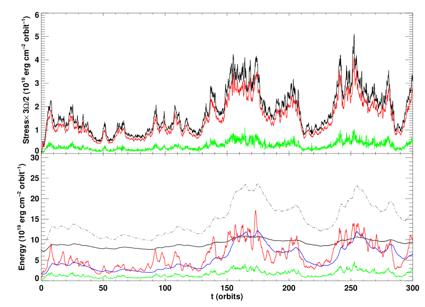
Figure 1: Volume-integrated stresses (upper panel) and energies (lower panel) in STD32 as a function of time. Top panel: Maxwell stress (red), Reynolds stress (green) and the sum of these two (black). Bottom panel: internal energy (black), radiation energy (blue), $10$ times the magnetic energy (red), $10$ times the kinetic energy(green) and total energy (grey dash-dotted). The quantities are all vertically integrated and the stress is multipled by $3\Omega/2$.

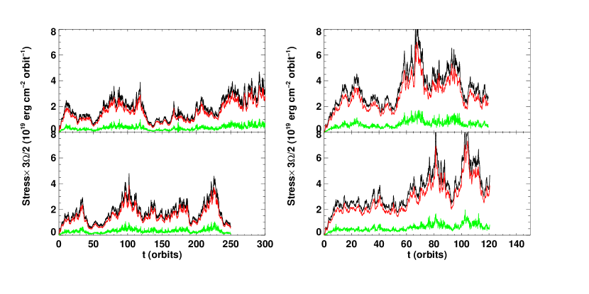
Figure 2: Volume-integrated stresses in Y128(upper left panel), X64(lower left panel), Z512(upper right panel) and DBLE(lower right panel) as a function of time. The color curves are coded as in the top panel of Fig.1.

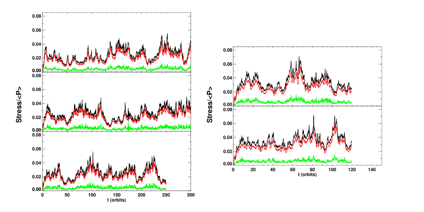
Figure 3: Volume-integrated stresses in ratio to simultaneous volume-averaged total pressure for STD32, Y128, X64 (left, from top to bottom), Z512 and DBLE (right, from top to bottom). Color code is the same as in Fig.2.

We are primarily interested in time-averaged quantities representative of conditions in a steady-state disk. To determine the appropriate time-averaging period, we examined how rapidly the effects of our initial conditions and transient response die away. As Figures 1, 2, and 3 show, in every simulation the various contributions to the stress reach levels characteristic of the statistical steady-state by $\sim 10$ orbits from the beginning. Topological properties of the initial magnetic field are erased rapidly: the net azimuthal flux changes sign on $\sim 5$ orbit timescales, and the volume-integrated magnetic helicity has a correlation time of at most $\sim 3$ orbits. We therefore defined each simulation’s time-average as beginning at 10 orbits and running to its end.

3.1 STANDARD RUN

We show the time evolution of the stresses and energies of STD32 in Fig.1. STD32 has the same resolution and nearly identical initial setup as the run in Hirose et al. (2006), which makes it easy to compare them statistically (note, however, that STD32 ran for five times as long). STD32 appears to have two stages after the transient decay, which separate around $130$ orbits. During the first stage, the maximum Maxwell stress is about $3$ times as great as the minimum, which is nearly the same as the gas pressure-dominated run in Hirose et al. (2006). The ratio of box-integrated stress to box-integrated total pressure (including both the gas and radiation pressures) is $0.015$, and that is also consistent with the value found in Hirose et al. (2006) (it was $0.016$ in their paper). In the second stage, the peak value of the stress doubles, and the range of the fluctuations is roughly a factor of $4$. A quick look at the radiation energy and gas energy plots in Fig.1 reveals that although the disk starts as a gas pressure-dominated system, it gradually evolves toward a situation with a larger ratio of radiation to gas pressure: the time- and volume-averaged ratio $\langle\langle p_{rad}\rangle/\langle p\rangle\rangle$ is $\sim 0.2$ for the first $130$ orbits, but increases to $\sim 0.4$ for the rest with a variation range $\simeq 0.2-0.5$. Here the first (inner) $\langle\rangle$ represents a volume average and the second (outer) denotes a time average. Comparison with the previous simulation with comparable gas and radiation pressure (Krolik et al., 2007) is helpful. In that run, the variation of the stress is $\sim 6$, which is slightly bigger than that of the second stage of STD32; the nominal time-averaged $\alpha$-parameter is $\simeq 0.03$, while it is a bit smaller, $\sim 0.02$, for STD32; the ratio of radiation pressure to gas pressure varies over the range $\simeq 0.5-2$, which is beyond that of STD32. Despite large fluctuations, STD32 clearly achieves a quasi-stable stage for the last $150$ orbits. All other four runs in this paper also show the feature of increasing $\langle p_{rad}\rangle/\langle p\rangle$, and they are terminated when a quasi-stable stage like the one in STD32 is reached.

3.2 CONVERGENCE

The saturation states of the other four runs are illustrated in Fig.2. Clearly the saturation level of X64 and Y128 (left two panels in the graph) are similar while the Z512 and DBLE (right two panels) have relatively higher mean values. The offset between the left two and the right two begins right after the transient decay. It grows even larger after the first $60$ orbits in both Z512 and DBLE: at that point, the radiation energy becomes comparable with the gas energy.

To study convergence quantitatively, we need not only temporal and spatial averages of the stress, but proper ways to normalize it. Here we choose the averaging time to be from the end of the transient phase ($10$ orbits) to the end of the run; the volume-integral of the stress is used as the spatial average. Unlike the nonstratified case, the pressures in our simulations show both consistent spatial gradients, depending on height from the midplane, and significant trends over time. We therefore employ three different methods of normalization, and examine the quality of numerical convergence in each case.

We first normalize the different kinds of stress and energy by the initial volume-averaged total pressure $P_{0}$ (sum of gas pressure and radiation pressure): $P_{0}=9.36\times 10^{11}$ ergs cm^-3 in our simulations. This normalization definition is extensively used in unstratified shearing box simulations, but with the total pressure replaced by thermal pressure alone. The time- and box-averaged values are given in Table 1. Scanning across each line, one can see which quantities are sensitive to resolution; in general, convergence has clearly been reached with regard to $x$ and $y$ cell size, but not with respect to $\Delta z$. The normalized Maxwell stress is constant at $\simeq 0.03$ when the resolution in the radial or azimuthal directions increases, but its value is almost doubled when the vertical resolution is raised by a factor of $2$. Similarly, the magnetic energy and turbulent kinetic energy rise by about a factor of two when the vertical cell count is doubled, but are independent of the horizontal cell dimensions. By contrast, in unstratified simulations, when the resolution improves, the saturation level either decreases toward zero with a zero net-field configuration (Fromang & Papaloizou, 2007; Simon et al., 2009) or increases weakly for mean azimuthal field models (Guan et al., 2009). We have net azimuthal field in our simulations, but it is not fixed, and even the sign of the net azimuthal flux changes.

A second useful normalization standard is the horizontal average of the time-dependent total pressure in the midplane. The time-averaged values for the stresses and energies normalized in this fashion are listed in Table 1, too. They depend on resolution in a way very similar to the ones using the absolute normalization except that their values are almost one order of magnitude smaller. Again, in this normalization there is no dependence on horizontal resolution, but increasing resolution in $z$ leads to larger values. For example, the Maxwell stress for DBLE is almost twice that of STD32.

Considering that $P_{0}$ is just an arbitrary initial guess for the total pressure, and $P(0)$ does not reflect the properties of the whole box, it is more physical to normalize the energies and stresses to the simultaneous volume-averaged total pressure, i.e., $\langle P\rangle\equiv\langle p_{rad}+p\rangle$. The time evolution curves of the stress ratios using this normalization are plotted in Fig.3. Compared to the absolute stresses shown in Fig.1 and 2, the stress ratios after normalization show considerably smaller peak-to-peak variations. Normalized in this way, there is also a significantly smaller increase when the resolution along the vertical direction increases. The time averaged values for this normalization are the third group in Table 1. The normalized Maxwell stress is $\sim 0.02$ for STD32, X64 and Y128, and increases only to $\simeq 0.03$ for Z512 and DBLE. This sort of normalization is the best of the three to use for estimating the Shakura-Sunyaev $\alpha$ parameter because it makes use of the actual volume-integrated total pressure, and we see that with the best resolution employed here, we are approaching convergence in defining its value. We emphasize, however, that one can speak of a single value for this number only in terms of a particular location in the disk and after both a vertical integration and a time average that encompasses many thermal times.

To summarize this section, we find that numerical convergence with respect to resolution in the $x$ and $y$, but not $z$, directions has been achieved for the absolute values of stress and energy in a stratified shearing box. Increasing $z$ resolution at the level we have reached leads to rising absolute values of stress and pressure. On the other hand, we come close to reaching convergence with respect to all three sorts of resolution for the ratio of stresses and energies to the time-dependent total pressure. In the next subsection, we show that certain detailed features of the magnetic field show similar convergence properties and cast light on why stratified shearing boxes differ from unstratified.

3.3 FIELD STRUCTURE

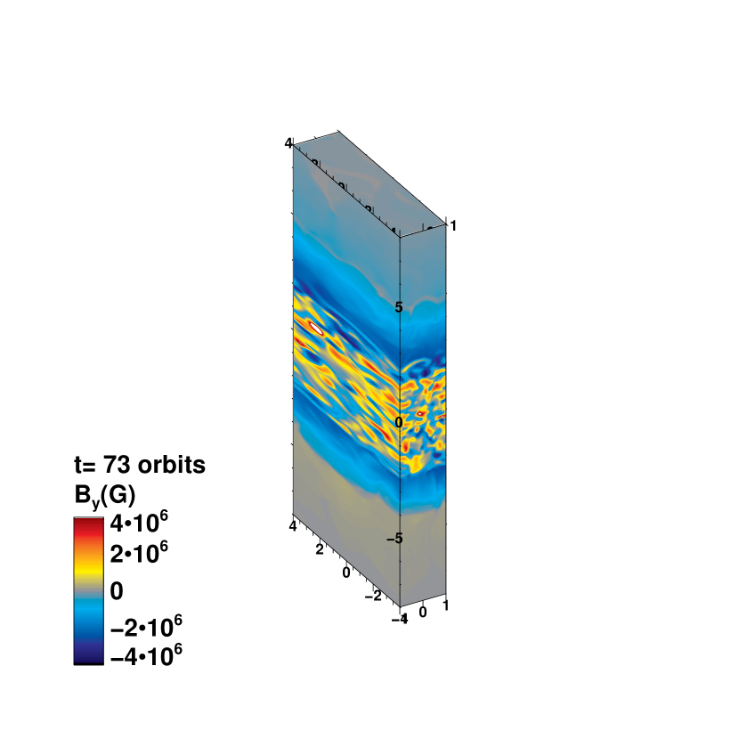
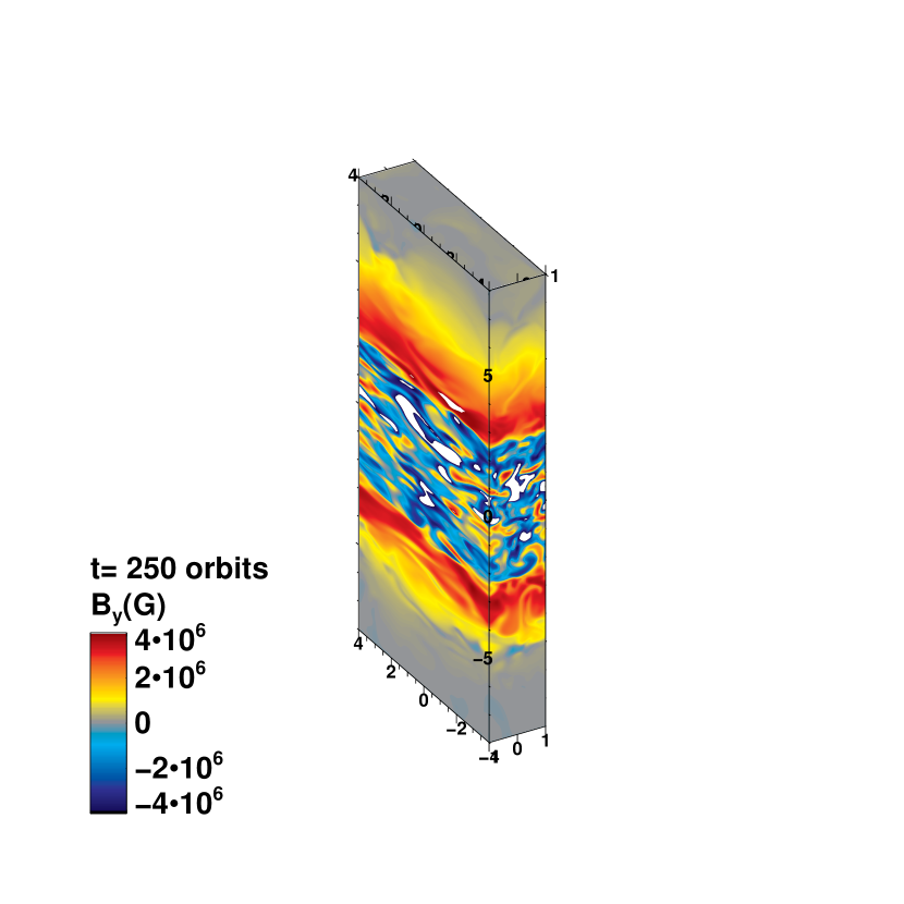
Figure 4: Snapshots of the $B_{y}$ distribution on the box surfaces at $t=73$ orbits and $t=250$ orbits in STD32.

In order to investigate the effect of stratification on the magnetic field, we consider the vertical correlation length of the field. As the azimuthal component dominates in our simulations, we restrict our attention to $B_{y}$. We present two 3-D snapshots of the distribution of azimuthal field strength in STD32 in Fig. 4. In the plot, color contours of the field strength are mapped onto the surfaces of the box. For contrast, we choose a pair of times, one ($t=73$ orbits) when the magnetic energy is low and one ($t=250$ orbits) when it is high. We find the field distribution below $\pm 2H$ of height is distinct from that above: within that distance of the midplane, the field is turbulent, whereas at higher altitudes it is much more regular. Far from the midplane, long filamentary regions of relatively smooth $B_{y}$ with the same sign extend more than 1–$2H$ beyond the disk core. The field becomes disordered again above $\sim\pm 5H$, where the sign of $B_{y}$ sometimes flips. The same features are consistently observed in all our other runs. Stratification clearly has a strong effect on the qualitative organization of the magnetic field.

This fact leads us to ask if stratification also influences the field structure of the midplane region. Let us first calculate the physical scale height by taking $\langle c_{s}/\Omega\rangle$. The time averaged scale height is then denoted as $\mathcal{H}$ hereafter. This scale height is a better measure of the physical scale length of the disk than our guessed unit of length, $H$. The physical scale height varies within the range $\simeq 1.4$–$2H$ for STD32, with time average $1.65H$ (similar variations and average values are also found in X64 and Y128, see Table 1); its range of variation is slightly wider, $\simeq 1.4$–$2.3H$ in Z512 and DBLE, and the average is also a bit larger, $\sim 2.0H$.

We now calculate the vertical correlation length of $B_{y}$ in the disk core, which we define as $|z|\leq H$, i.e. within roughly half a physical scale height of the midplane. This choice allows us to compare our results with those of Fromang & Papaloizou (2007), whose box extended one physical scale height vertically. Note that our DBLE run has exactly the same resolution as their STD64 (both are $\mathcal{H}/64$ vertically). The two-point correlation function of $B_{y}$ at $t=t_{0}$ is defined as:

$$C_{z}(B_{y};t_{0},l_{z})\equiv\frac{1}{L_{x}L_{y}}\int\!\!\!\int dxdy~{}\frac{\int B_{y}(t_{0},x,y,z)B_{y}(t_{0},x,y,z-l_{z})dz}{\int B_{y}^{2}(t_{0},x,y,z)dz},$$ (1)

where $C_{z}(B_{y};t_{0},l_{z})$ denotes the vertical correlation of $B_{y}$ at separation $l_{z}$ as a function of time, and $L_{x}$ and $L_{y}$ are the box sizes along the $x$ and $y$ directions. Following Fromang & Papaloizou (2007), we define an integrated correlation length as the integral over different separations:

$$\lambda_{z,~{}int}(B_{y};t_{0})=\int C_{z}(B_{y};t_{0},l_{z})~{}dl_{z}.$$ (2)

Note that in Fromang & Papaloizou (2007) the correlation length is calculated only in the $x-z$ plane. We find that our value of the integrated correlation length would change by only $\sim 3\%$ (see Table 1) if we had used their definition instead of ours. We also calculate the correlation length defined as the full width at half maximum (FWHM) of $C_{z}$, i.e.,

$$\lambda_{z,~{}FWHM}(B_{y};t_{0})=\textrm{FWHM~{}of~{}}C_{z}(B_{y};t_{0},l_{z}).$$ (3)

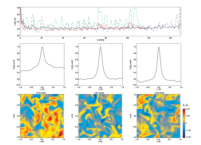
Figure 5: Top: Radially averaged vertical correlation length of $B_{y}$ for STD32 (black solid for $\lambda_{z,~{}FWHM}$ and blue dashed for $\lambda_{z,~{}int}$) and DBLE (red solid for $\lambda_{z,~{}FWHM}$ and green dash-dotted for $\lambda_{z,~{}int}$) as a function of time; Middle: The correlation function at $t=73$, $97$ and $25$ orbits of DBLE; Bottom: $B_{y}$ contours from DBLE in $y=0$ plane at $t=73$, $97$ and $25$ orbits.

We show the time histories for several definitions of $\lambda_{z}$ in STD32 and DBLE in the top panel of Fig. 5. As this figure shows, both the integrated and the FWHM correlation length vary with time, but $\lambda_{z,~{}int}$ has considerably larger fluctuations than $\lambda_{z,~{}FWHM}$. A close look at the correlation function explains the discrepancy. In the middle of the same graph, three instantaneous correlation functions, at $t=73$, $97$ and $25$ orbits in DBLE are presented. At $t=73$ orbits, $C_{z}(B_{y})$ clearly shows positive correlation even at large separations, making the integrated correlation length $\lambda_{z,~{}int}$ as large as $0.8H$, about twice the $\lambda_{z,~{}FWHM}$ found at the same time. On the other hand, at $t=25$ orbits, the correlation function turns negative when $|l_{z}|>0.3H$, and thus a dip of $\lambda_{z,~{}int}$ ($\sim 0.1H$) is observed at $t=25$ orbits, when $\lambda_{z,~{}FWHM}$ is $\sim 60\%$ large. The two measures of $\lambda_{z}$ become comparable to each other when the wings of $C_{z}(B_{y})$ asymptote to zero at larger separations. For example, at $t=97$ orbits, when this occurs, $\lambda_{z,~{}FWHM}$ is similar to, but slightly less than $\lambda_{z,~{}int}$. We can test whether $\lambda_{z,~{}int}$ or $\lambda_{z,~{}FWHM}$ is the more realistic measure of the correlation length by looking at snapshots of $B_{y}$, such as those shown under each correlation plot. There is no apparent change in the lengthscales of magnetic field features between $t=25$ and $97$ orbits, despite the factor of two change in the intergrated correlation length between those times. The FWHM correlation lengths at these two times are nearly the same. Thus, we claim that the FWHM definition is a better measure of the correlation length than the integrated version: it corresponds more closely to one’s visual impression and varies less in time. The large fluctuations in $\lambda_{z,~{}int}$ appear to be due to sensitivity to the tails of $C_{z}$.

As shown by the time averaged values listed in Table 1, $\lambda_{z,~{}FWHM}$ decreases slightly in magnitude when the resolution is doubled. We find $\langle\lambda_{z,~{}FWHM}\rangle_{t}\sim 0.26H$ for STD32, but drops to $\sim 0.22H$ once the $z-$cell number is doubled. This change corresponds to a $30\%$ decrease if we scaled the length with the physical scale height $\mathcal{H}$: $\langle\lambda_{z,~{}FWHM}\rangle_{t}\sim 0.16\mathcal{H}$ for STD32 and $\sim 0.11\mathcal{H}$ for DBLE. As we mentioned before, the DBLE run possesses the same resolution as STD64 in Fromang & Papaloizou (2007), in which the time averaged correlation length using their definition (an integrated one) is $0.06\mathcal{H}$; with the same definition, the correlation length of DBLE is $\sim 0.18\mathcal{H}$, approximately triple theirs.

In sum, we find comparatively large scale ($\gtrsim 1H$) structures in $B_{y}$ more than $\simeq 2H$ from the midplane, and even in the region quite close to the midplane, features several times larger than found in unstratified simulations. We also find that the FWHM definition of the vertical correlation length may be more useful than the integrated one. In terms of its degree of numerical convergence, $\lambda_{z}$ is similar to the ratio of stress to simultaneous pressure: at the resolution scales achieved in these simulations, it appears to be close to convergence, but not quite there, particularly with respect to resolution in the vertical direction.

3.4 MAGNETIC BUOYANCY

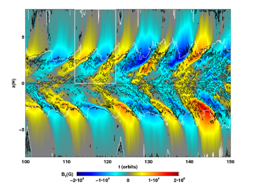
Figure 6: Spacetime diagram of the azimuthal component of the magnetic field. The contour lines on top delineate where and when the magnetic Brunt-Väisälä frequency squared (black) changes from positive (inside the contours) to negative (outside the contours) and the plasma $\beta$ (white) increases from less than unity (outside the contours) to greater (inside the contours). The white rectangle shows the section magnified in Fig.7.

As discussed in the last subsection, large filament-like structures of magnetic field emerge above the core of the disk and extend vertically for another $1-2H$. These features have also been observed in many previous simulations (e.g., Turner, 2004; Hirose et al., 2006). In Figure 6, we show a space-time diagram of the horizontally-averaged azimuthal component of the field from a 50-orbit segment of STD32. There are roughly ten episodes of field upwelling during this sample, corresponding to a period of $\sim 5$ orbits for the process. The sign of $B_{y}$ alternates in successive events. The upward pattern speed is $\sim 0.5H$ per orbit at the base of the plume ($\sim\pm 2H$), accelerating to $\sim 1-2H$ per orbit near the top of the disk ($\gtrsim\pm 4H$). These events are almost symmetrical about the midplane except for some small phase offsets and intensity variations.

Computing the simple hydrodynamic Brunt-Väisälä frequency for our data would suggest that the disk is always stable against buoyancy-driven instability below $\sim 2H$, and remains mostly stable at higher altitudes, including the upwelling regions. However, including magnetic forces leads to a very different result.

There are two magnetic buoyancy modes to consider: the interchange mode and the undulatory Parker instability. The former mode is not present in our simulations: evaluating its dispersion relation with horizontally averaged data shows that the disk is stable at nearly all times and in nearly all locations. To demonstrate that the undulatory mode does seem to be responsible for these repeated episodes of magnetic upwelling, we begin by writing down expressions for the square of the generalized magnetic Brunt-Väisälä frequency for this mode in two limits: fast and slow radiation diffusion (Tao & Blaes, 2009, in preparation):

$$N^{2}_{mag,fast}=\frac{gv_{A}^{2}}{c_{i}^{2}+v_{A}^{2}}\frac{d\ln{|\textbf{B}|}}{dz},$$ (4)

$$N^{2}_{mag,slow}=N^{2}_{hyd}+\frac{gv_{A}^{2}}{c_{t}^{2}}\frac{d\ln{|\textbf{B}|}}{dz}.$$ (5)

Here $N_{hyd}$ is the hydrodynamic Brunt-Väisälä frequency for a thermally coupled gas and radiation mixture (Blaes et al., 2007), $g=z\Omega^{2}$ is the vertical component of gravity, $v_{A}$ is the Alfvén speed, and $|\textbf{B}|$ is the magnitude of the field strength. The isothermal sound speed in the gas is $c_{i}=(p/\rho)^{1/2}$, and the total adiabatic sound speed is $c_{t}=[\Gamma_{1}(p+E/3)/\rho]^{1/2}$, where $p$ and $E$ again are gas pressure and radiation energy density, and $\Gamma_{1}$ is Chandrasekhar’s generalized adiabatic constant (Chandrasekhar, 1967). The “slow diffusion” limit describes the case in which the growth rate of the instability exceeds the photon diffusion rate so that photons are dynamically well-coupled to the fluid; in the “fast diffusion” limit, photons diffuse rapidly compared to the instability growth rate, so that there is no radiation pressure response to the mode and the perturbations in the gas are isothermal. Note that hydrostatic equilibrium with no magnetic tension forces is assumed in both expressions for $N^{2}_{mag}$. Evaluating the growth rate using the wavelength of the fastest-growing mode in the rapid diffusion limit (equation A15 of Blaes et al. (2007)), we find that, for regions above $\sim\pm 3.5H$, the fast diffusion limit is the appropriate one, while at lower altitudes the slow diffusion limit generally applies. In approximate terms, $N^{2}_{mag}$ can then be treated as the proper combination of the frequency squared under those two limits. The fastest-growing wavelength is always well confined in the box and well resolved numerically in most regions except near the midplane.

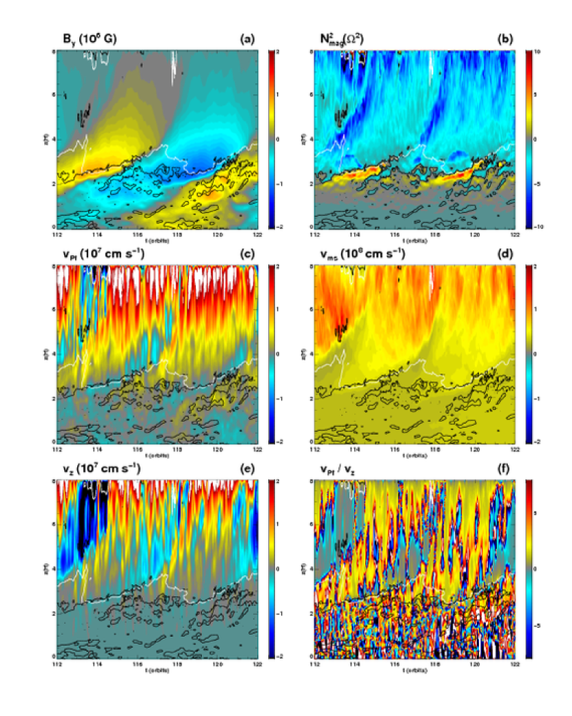
Figure 7: Magnified view of a portion of the spacetime diagram for STD32: (a) azimuthal magnetic field strength; (b) magnetic Brunt-Väisälä frequency squared; (c) vertical velocity of the Poynting flux; (d) magnetosonic speed; (e) vertical gas velocity; (f) ratio of the Poynting flux velocity to the vertical gas velocity. See legend on the top of each panel for units. The black and white contour lines are the same as in Fig.6.

We plot the zero-frequency contour of the combined $N^{2}_{mag}$ (black curves) in the space-time diagram of Figure 6. Instability takes place only outside the contour lines. Inside $\pm 2H$, i.e. the core disk region, this mode is generally stable, although sometimes only marginally so. Small unstable patches exist in the core region, and most of them are elongated in a way suggesting buoyancy, but they exist only briefly. The magnitude of the growth rate in this region is small (see panel b of Fig. 7), and the implied rise speeds are relatively slow. These small episodes of unstable buoyancy may help explain why we find larger scale features in our stratified simulations than have been found in unstratified simulations, but the fact that the wavelength of the fastest-growing modes exceeds the size of the box suggests that this explanation probably cannot completely answer the question of the origin of our larger correlation length. On the other hand, $N^{2}_{mag}$ is negative almost everywhere at altitudes above $\sim\pm(2$–$3)H$. At these higher altitudes, the undulatory Parker mode is almost always unstable with a linear growth rate $\sim(1$–$2)\Omega$.

In order to show the operation of this mechanism in greater detail, we study a magnified view of a small domain of the spacetime diagram. Data from the region within the white rectangle in Figure 6 are displayed on a larger scale in Figure 7. As discussed, the rising pattern is roughly symmetric about the midplane, so by choosing a sample from the upper half of the disk we should not lose any interesting physics. The time range of this sample is $10$ orbits and contains almost two complete buoyancy episodes. In this figure, we plot not only $B_{y}$ and $N^{2}_{mag}$, but also three characteristic speeds: the gas vertical velocity $v_{z}$, the magnetosonic speed $v_{ms}$, and the Poynting flux speed $v_{P\!f}$. The last one is defined as $v_{P\!f}\equiv 4\pi S_{z}/B^{2}$, where $S_{z}$ represents the $z$ component of the Poynting flux. Thus, positive $v_{P\!f}$ means field energy is transported upward and corresponds to field ascending. The Poynting flux speed can also be written as $v_{P\!f}=v_{z}-(\textbf{v}\cdot\textbf{B})B_{z}/|\textbf{B}^{2}|$; this form shows how, even in the MHD limit, the gas and magnetic velocities can differ to the extent that the fluid can slide along field lines.

Panels a, c, and e of Figure 7 present an enlightening contrast: although the magnetic field spacetime diagram consistently shows features in $B_{y}$ rising upward from near the midplane all the way to the top of the box, the $v_{P\!f}$ and $v_{z}$ illustrations demonstrate that consistent upward field and fluid motion begins only at $\simeq 3H$ above the midplane. In fact, the bottom edge of the true upwelling region corresponds closely to the lower boundary of the Parker instability region. Thus we see that the apparent motion of regions of strong field in the disk core and lower corona is a wave or pattern motion almost completely divorced from genuine mass or field transport. In fact, the pattern speeds observed in the simulation are close to the Alfvén speed, suggesting that the waves in question are either Alfvén or slow magnetosonic waves. The latter mode appears to be particularly important for short-wavelength, high-frequency variability, for which a distinct anti-correlation between magnetic and gas pressure fluctuations can be seen.

As already remarked, genuine rising motion of magnetic field and gas is closely associated with the onset of magnetic buoyancy instability. Further evidence that undulatory Parker mode instability is the origin of upwelling is provided by the fact that the regions of greatest growth rate (the dark blue strips in the $N^{2}_{mag}$ panel) coincide with the leading edges of regions where both $v_{P\!f}$ and $v_{z}$ are large. In other words, the acceleration to high upward velocity takes place where the instability grows most strongly.

Although true upward motion certainly takes place at altitudes several scale heights from the midplane, it is in an absolute sense relatively slow. Typical speeds for both $v_{P\!f}$ and $v_{z}$ are $\sim(0.08$–$0.8)\mathcal{H}\Omega$. Both are subsonic, only $\sim O(0.1)v_{ms}$ (note that the units in the $v_{ms}$ panel are $10^{8}$ cm s^-1 rather than the $10^{7}$ cm s^-1 of the $v_{P\!f}$ and $v_{z}$ panels). The slowness of these speeds demonstrates that even though much of the corona is buoyantly unstable, the net accelerations are never more than a fraction of gravity.

The relationship between $v_{P\!f}$ and $v_{z}$ changes sharply between the disk core and the corona, as can be seen in panel f of Figure 7, which shows their ratio. In the disk core, they are entirely uncorrelated, consistent with our conclusion that there are no genuine flows of either in that part of the disk. On the other hand, in the coronal region, $|z|>2H$, although not strictly proportional, more often than not they vary together, with $v_{P\!f}\simeq(1$–$2)v_{z}$. Where the undulatory Parker mode grows, field lines develop upward bends and can carry gas upward with them. However, the curvature of the field lines permits the gas to slip diagonally downward relative to the field, an effect explaining why the mean upward speed for gas is smaller than that for field.

To sum up, we find that the undulatory Parker instability is the major driver of the magnetic upwelling that has been so often noted in stratified shearing box simulations. Most of the time, it is marginally stable in the core region ($|z|\lesssim 2H$), and unstable above it. Consistent upward mass and field motions begin only at the lower boundary of the Parker instability, and both of them are one order of magnitude slower than the magnetosonic speed. The upward velocity of gas motion is generally half of the field flux velocity as the gas may slide towards the field line valleys.

3.5 Geometry of turbulent eddies

The turbulence produced by the MRI is frequently described in the literature as “horizontal” because the initial work on shearing boxes found that the kinetic energy of turbulent motions in the $x-$ and $y-$ directions, corresponding to the radial and azimuthal directions if the box were placed in an actual disk, was substantially greater than that in the $z-$, or vertical, direction. For example, Hawley et al. (1995) found that in their fiducial simulation of a three-dimensional, but unstratified, shearing box (in this case, with initial magnetic field uniform and vertical), $\langle\rho v_{x}^{2}\rangle\simeq\langle\rho(\delta v_{y})^{2}\rangle\simeq 4\langle\rho v_{z}^{2}\rangle$, where $\delta v_{y}$ is the y-velocity after subtracting out the shearing motion. An initially azimuthal field also led to primarily horizontal motions, although with somewhat larger amplitude in the radial than in the azimuthal direction. Similarly, in a stratified shearing box that extended $\pm 2\sqrt{2}{\cal H}$ from the midplane, Stone et al. (1996) found that the turbulence was predominantly azimuthal: $\langle\rho(\delta v_{y})^{2}\rangle\simeq 6\langle\rho v_{x}^{2}\rangle\simeq 20\langle\rho v_{z}^{2}\rangle$, with little dependence on whether the equation of state was isothermal or adiabatic or on whether the initial field was vertical or azimuthal.

However, the situation changes when stratified shearing boxes with greater vertical extent are simulated, and the periodic boundary conditions used by Stone et al. (1996) are replaced by outflow boundary conditions. Miller & Stone (2000) reported that in their simulations, in which the box extended to $\pm 5\sqrt{2}{\cal H}$ from the midplane, the amplitude of vertical motion near the midplane ($|z|\leq 2\sqrt{2}{\cal H}$) was almost as great as the amplitude of the azimuthal turbulent motions: $\langle\rho(\delta v_{y})^{2}\rangle\simeq 1.2\langle\rho v_{z}^{2}\rangle$, nearly independent of whether the initial field was vertical or azimuthal. Their result for the ratio $\langle\rho v_{z}^{2}\rangle/\langle\rho v_{x}^{2}\rangle$ was more ambiguous: its value was $\simeq 0.5$ when the initial field was azimuthal, but fell to $\simeq 0.27$ when it was vertical. Our results are qualitatively similar to those of Miller & Stone (2000), but indicate turbulent motions that are more nearly isotropic. Averaging the standard resolution data over time and the region within $\pm 2H$ of the midplane, we have $\langle\rho(\delta v_{y})^{2}\rangle\simeq 0.70\langle\rho v_{x}^{2}\rangle\simeq 1.2\langle\rho v_{z}^{2}\rangle$. In the highest-resolution simulation, the azimuthal motions grow slightly relative to both the radial and vertical motions, but overall, all three velocity components remain comparable in magnitude: $\langle\rho(\delta v_{y})^{2}\rangle\simeq 0.90\langle\rho v_{x}^{2}\rangle\simeq 1.6\langle\rho v_{z}^{2}\rangle$. That such a qualitative contrast in the geometry of turbulent motions is associated with the change from unstratified to stratified boxes strongly suggests that its physical origin can be identified with the principal physical contrast between the two cases: vertical gravity, which in this context drives magnetic buoyancy.

4 CONCLUSIONS

We have shown that in a stratified shearing box, unlike an unstratified one, the magnetic saturation level does not diminish with increasing grid resolution. Instead, at the resolutions used in our simulations, the Maxwell stress is independent of the $x$ and $y$ resolution. When the vertical resolution increases, both the stress and the pressure grow. Despite the nearly linear increase of both magnetic stress and total pressure with resolution ($\langle B_{r}B_{\phi}\rangle,\langle P\rangle\propto(\Delta z)^{-1}$), the ratio of stress to pressure is almost converged at this resolution (as also found in the isothermal simulations of Davis et al. (2009)), increasing only slowly with finer vertical resolution.

The field structure of a stratified box is quite different from that of an unstratified box. At high altitude ($|z|>2H$), the field is dominated by its azimuthal component and forms smoothly distributed filamentary structures with vertical thicknesses $\gtrsim H$. In the core of the disk, the region unstratified boxes are thought to mimic, the field is turbulent, but with significantly larger scale features than found in unstratified simulations: for simulations with identical resolution, the vertical correlation length of $B_{y}$ is $\sim 3$ times greater with vertical gravity than without. In addition, when gravity is present, the correlation length measured at this resolution is much less dependent on gridscale, falling only $\simeq 30\%$ when the resolution is doubled.

There are several ways to understand the contrast between magnetic field behavior in the stratified and unstratified cases. One is through dimensional analysis. Without vertical gravity, the ratio $c_{s}/\Omega$, although well-defined, loses its physical significance. Consequently, the only remaining significant lengthscale in the problem is the gridscale. As a result, the two lengthscales determined by the turbulence, the field correlation length and $v_{A}/\Omega$, both track the gridscale and approach zero as the resolution grows finer. On the other hand, with vertical gravity, $c_{s}/\Omega$ plays an explicit role in the turbulent dynamics, and both the field correlation length and $v_{A}/\Omega$ can become associated with it. A related argument has been made by Vishniac (2009).

A second approach ties the result more directly to gravitational dynamics. As we have shown, buoyancy plays an important role in the character of MRI-driven MHD turbulence in stratified shearing boxes. Outside the midplane region ($|z|\geq\pm(2$–$3)H$), $N^{2}_{mag}$ is consistently negative, a signal that buoyant regions are continually being created. Consequently, at any given time there is nearly always a rising magnetic filament in that region. Even inside the midplane region, vertical motions, presumably excited by the buoyantly-driven pressure fluctuations on its edges, are greater than they are in unstratified situations. In notable contrast to studies of both unstratified shearing boxes and stratified shearing boxes with periodic vertical boundary conditions and containing only a few vertical scale heights, we find that the turbulent motions are fully three-dimensional, with the kinetic energy in vertical motion comparable to that in either of the horizontal directions.

Because fully three-dimensional motion is essential to dynamo action (e.g., as reviewed by Cowling (1981) and first emphasized in this context by Brandenburg et al. (1995)), the buoyant excitation of vertical motion is essential to maintaining the magnetic field: as fluid elements rise and fall, they create vertical field from horizontal. The pressure scale height sets the characteristic scale for vertical motions, linking the magnitude of the field (with proportionality constant $\sim\sqrt{4\pi\rho}\Omega$) to this characteristic lengthscale (see Vishniac (2009) for a proposed scaling relation). At saturation, field amplification by dynamo action is balanced by two field loss mechanisms: dissipation and expulsion of field from the box. As previously shown by Hirose et al. (2006), the former strongly dominates the latter when allowance is made for photon energy losses.

We have also used these simulations to identify the dynamical mechanism responsible for the upward magnetic motions commonly seen in previous stratified simulations: it is the undulatory Parker instability. This mode is marginally stable within the core region, but is almost always unstable outside that region. True upward motions of both magnetic field and fluid begin at the instability boundary, but are one order of magnitude slower than the magnetosonic speed. Because the gas can slide along field lines and fall into field line valleys, its mean upward velocity is generally only about half the Poynting velocity.

Although we have allayed fears that the true converged state of MRI-driven MHD turbulence is zero stress, the question of numerical convergence of the stratified case remains open. We understand neither why the stress and pressure are strongly dependent on vertical (but not horizontal) cell size nor at what resolution this dependence may weaken. The origin of the large fluctuations as a function of time observed in box-integrated quantities in these simulations is also unclear, although there are hints that their magnitude may have to do with the radial width of the box (e.g., Fromang & Stone, 2009).

Several physical questions also remain unanswered: The pressure scale height certainly sets a physical lengthscale, but can we understand more specifically how it determines the vertical correlation length in the disk core’s MHD turbulence? It seems plausible that the field buoyancy leads to larger scale features in the core region, as the field senses the vertical outflow boundaries via the magnetic upwelling, but exactly how is that communicated to the midplane? Lastly, one of the most striking features of the disk corona is the quasi-regular alternation in sign of $B_{y}$: what causes this alternation and what determines its characteristic lengthscale and timescale?

Table 1: Properties of the simulations in the paper.

	STD32	X64	Y128	Z512	DBLE
resolution	$32\times 64\times 256$	$64\times 64\times 256$	$32\times 128\times 256$	$32\times 64\times 512$	$64\times 128\times 512$
Run time (orbits)	300	250	300	120	120
$\Delta\Sigma_{max}/\Sigma~{}(\%)$	2.5	2.0	2.0	1.1	1.4
$\mathcal{H}=\langle\langle c_{S}/\Omega\rangle\rangle~{}(H)$	$1.65$	$1.67$	$1.67$	$2.00$	$1.94$
$\langle\langle t_{cool}\rangle\rangle$ (orbits)	$8.0$	$7.8$	$7.7$	$6.6$	$6.3$
$\langle\lambda_{z,~{}int}(B_{y})\rangle_{t}~{}(H)$	$0.31$	$0.35$	$0.34$	$0.35$	$0.34$
$\langle\lambda_{z,~{}int}(B_{y};y=0)\rangle_{t}~{}(H)$	$0.31$	$0.36$	$0.33$	$0.35$	$0.33$
$\langle\lambda_{z,~{}FWHM}(B_{y})\rangle_{t}~{}(H)$	$0.26$	$0.25$	$0.25$	$0.23$	$0.22$
$\langle\langle-B_{x}B_{y}/4\pi\rangle\rangle/P_{0}$	$0.029$	$0.030$	$0.031$	$0.064$	$0.060$
$\langle\langle\rho v_{x}\delta v_{y}\rangle\rangle/P_{0}$	$6.7\times 10^{-3}$	$6.7\times 10^{-3}$	$7.0\times 10^{-3}$	$0.015$	$0.013$
$\langle\langle B^{2}/8\pi\rangle\rangle/P_{0}$	$0.11$	$0.11$	$0.11$	$0.24$	$0.20$
$\langle\langle B^{2}_{x}/8\pi\rangle\rangle/P_{0}$	$9.1\times 10^{-3}$	$9.3\times 10^{-3}$	$0.010$	$0.025$	$0.024$
$\langle\langle B^{2}_{y}/8\pi\rangle\rangle/P_{0}$	$0.095$	$0.090$	$0.096$	$0.21$	$0.16$
$\langle\langle B^{2}_{z}/8\pi\rangle\rangle/P_{0}$	$5.9\times 10^{-3}$	$6.8\times 10^{-3}$	$6.5\times 10^{-3}$	$0.014$	$0.015$
$\langle\langle\rho\delta v^{2}/2\rangle\rangle/P_{0}$	$0.029$	$0.031$	$0.031$	$0.061$	$0.057$
$\langle\langle\rho v^{2}_{x}/2\rangle\rangle/P_{0}$	$0.012$	$0.012$	$0.012$	$0.024$	$0.021$
$\langle\langle\rho\delta v^{2}_{y}/2\rangle\rangle/P_{0}$	$0.010$	$0.011$	$0.011$	$0.023$	$0.023$
$\langle\langle\rho v^{2}_{z}/2\rangle\rangle/P_{0}$	$7.4\times 10^{-3}$	$8.0\times 10^{-3}$	$7.6\times 10^{-3}$	$0.014$	$0.014$
$\langle\langle-B_{x}B_{y}/4\pi\rangle/P(0)\rangle$	$3.9\times 10^{-3}$	$4.0\times 10^{-3}$	$4.1\times 10^{-3}$	$7.1\times 10^{-3}$	$7.3\times 10^{-3}$
$\langle\langle\rho v_{x}\delta v_{y}\rangle/P(0)\rangle$	$8.8\times 10^{-4}$	$8.8\times 10^{-4}$	$9.2\times 10^{-4}$	$1.7\times 10^{-3}$	$1.5\times 10^{-3}$
$\langle\langle B^{2}/8\pi\rangle/P(0)\rangle$	$0.014$	$0.014$	$0.015$	$0.040$	$0.024$
$\langle\langle B^{2}_{x}/8\pi\rangle/P(0)\rangle$	$1.2\times 10^{-3}$	$1.2\times 10^{-3}$	$1.3\times 10^{-3}$	$2.7\times 10^{-3}$	$2.9\times 10^{-3}$
$\langle\langle B^{2}_{y}/8\pi\rangle/P(0)\rangle$	$0.012$	$0.012$	$0.013$	$0.036$	$0.020$
$\langle\langle B^{2}_{z}/8\pi\rangle/P(0)\rangle$	$7.7\times 10^{-4}$	$8.8\times 10^{-4}$	$8.5\times 10^{-4}$	$1.4\times 10^{-3}$	$1.9\times 10^{-3}$
$\langle\langle\rho\delta v^{2}/2\rangle/P(0)\rangle$	$3.8\times 10^{-3}$	$4.1\times 10^{-3}$	$4.0\times 10^{-3}$	$6.7\times 10^{-3}$	$6.9\times 10^{-3}$
$\langle\langle\rho v^{2}_{x}/2\rangle/P(0)\rangle$	$1.6\times 10^{-3}$	$1.6\times 10^{-3}$	$1.6\times 10^{-3}$	$2.7\times 10^{-3}$	$2.6\times 10^{-3}$
$\langle\langle\rho\delta v^{2}_{y}/2\rangle/P(0)\rangle$	$1.3\times 10^{-3}$	$1.4\times 10^{-3}$	$1.4\times 10^{-3}$	$2.5\times 10^{-3}$	$2.8\times 10^{-3}$
$\langle\langle\rho v^{2}_{z}/2\rangle/P(0)\rangle$	$9.7\times 10^{-4}$	$1.0\times 10^{-3}$	$1.0\times 10^{-4}$	$1.5\times 10^{-4}$	$1.6\times 10^{-4}$
$\langle\langle-B_{x}B_{y}/4\pi\rangle/\langle P\rangle\rangle$	$0.020$	$0.021$	$0.021$	$0.029$	$0.029$
$\langle\langle\rho v_{x}\delta v_{y}\rangle/\langle P\rangle\rangle$	$4.6\times 10^{-3}$	$4.6\times 10^{-3}$	$4.7\times 10^{-3}$	$6.8\times 10^{-3}$	$6.3\times 10^{-3}$
$\langle\langle B^{2}/8\pi\rangle/\langle P\rangle\rangle$	$0.075$	$0.073$	$0.076$	$0.13$	$0.098$
$\langle\langle B^{2}_{x}/8\pi\rangle/\langle P\rangle\rangle$	$6.1\times 10^{-3}$	$6.4\times 10^{-3}$	$6.8\times 10^{-3}$	$0.011$	$0.012$
$\langle\langle B^{2}_{y}/8\pi\rangle/\langle P\rangle\rangle$	$0.064$	$0.062$	$0.065$	$0.11$	$0.079$
$\langle\langle B^{2}_{z}/8\pi\rangle/\langle P\rangle\rangle$	$4.0\times 10^{-3}$	$4.6\times 10^{-3}$	$4.3\times 10^{-3}$	$5.9\times 10^{-3}$	$7.5\times 10^{-3}$
$\langle\langle\rho\delta v^{2}/2\rangle/\langle P\rangle\rangle$	$0.020$	$0.021$	$0.021$	$0.028$	$0.028$
$\langle\langle\rho v^{2}_{x}/2\rangle/\langle P\rangle\rangle$	$8.2\times 10^{-3}$	$8.3\times 10^{-3}$	$8.5\times 10^{-3}$	$0.011$	$0.010$
$\langle\langle\rho\delta v^{2}_{y}/2\rangle/\langle P\rangle\rangle$	$6.8\times 10^{-3}$	$7.6\times 10^{-3}$	$7.3\times 10^{-3}$	$0.010$	$0.011$
$\langle\langle\rho v^{2}_{z}/2\rangle/\langle P\rangle\rangle$	$5.1\times 10^{-3}$	$5.5\times 10^{-3}$	$5.2\times 10^{-3}$	$6.3\times 10^{-3}$	$6.7\times 10^{-3}$
$\langle\langle-B_{x}B_{y}/4\pi\rangle/\langle B^{2}/8\pi\rangle\rangle$	$0.27$	$0.28$	$0.28$	$0.21$	$0.31$
$\langle\langle-B_{x}B_{y}/4\pi\rangle/\langle\rho v_{x}\delta v_{y}\rangle\rangle$	$4.6$	$4.7$	$4.5$	$4.4$	$4.8$
$\langle\langle-B_{x}B_{y}/4\pi\rangle\rangle/\langle\langle B^{2}/8\pi\rangle\rangle$	$0.26$	$0.27$	$0.28$	$0.27$	$0.30$
$\langle\langle-B_{x}B_{y}/4\pi\rangle\rangle/\langle\langle\rho v_{x}\delta v_{y}\rangle\rangle$	$4.3$	$4.5$	$4.4$	$4.3$	$4.6$

References

- Balbus & Hawley (1991) Balbus, S.A. & Hawley, J.F. 1991, 376, 214
- Balbus & Hawley (1998) Balbus, S.A., & Hawley, J.F. 1998, Rev. Mod. Phys., 70, 1
- Blaes et al. (2007) Blaes, O., Hirose, S. & Krolik, J.H. 2007, ApJ,664, 1057
- Brandenburg et al. (1995) Brandenburg,A. et al. 1995, ApJ, 446, 741
- Chandrasekhar (1967) Chandrasekhar, S. 1967, An Introduction to the Study of Stellar Structure (New York: Dover)
- Fromang & Papaloizou (2007) Fromang, S. & Papaloizou, J. 2007, A&A, 476, 1113
- Fromang et al. (2007) Fromang, S. et al. 2007, A&A, 476,1123
- Fromang & Stone (2009) Fromang, S. & Stone, J.M.,astro-ph 09064422
- Guan et al. (2009) Guan, X. et al. 2009, ApJ, 694, 1010
- Hawley et al. (1995) Hawley, J.F., Gammie, C.F., & Balbus, S.A. 1995, ApJ, 440, 742
- Hirose et al. (2006) Hirose, S., Krolik, J.H., & Stone, J.M. 2006, ApJ, 640, 901
- Hirose et al. (2009) Hirose, S., Krolik, J.H., & Blaes, O. 2009, ApJ, 691, 16
- Krolik et al. (2007) Krolik, J.H., Hirose, S., & Blaes, O. 2007, ApJ, 664, 1045
- Lesur & Longaretti (2007) Lesur, G. & Longaretti, P.-Y. 2007, MNRAS, 378, 1471
- Miller & Stone (2000) Miller, K.A. & Stone, J.M. 2000, ApJ, 534, 398
- Shakura & Sunyaev (1973) Shakura, N.I. & Sunyaev, R.A. 1973, A&A, 24, 337
- Simon et al. (2009) Simon, J.B., Hawley, J.F. & Beckwith, K. 2009, ApJ, 690, 974
- Stone et al. (1996) Stone, J.M., Hawley, J.F., Gammie, C.F., & Balbus, S.A. 1996, ApJ, 463, 656
- Tao & Blaes (2009) Tao, T. & Blaes, O. 2009, in preparation
- Turner (2004) Turner, N.J. 2004, ApJ, 605, 45
- Vishniac (2009) Vishniac, E.T. 2009, ApJ, 696, 1021
- Cowling (1981) Cowling, T.G. 1981, ARAA, 19, 115
- Davis et al. (2009) Davis, S.W., Stone, J.M. & Pessah, M. 2009, arXiv 0909.1570