Scaling laws of human interaction activity

Abstract

Even though people in our contemporary, technological society are depending on communication, our understanding of the underlying laws of human communicational behavior continues to be poorly understood. Here we investigate the communication patterns in two social Internet communities in search of statistical laws in human interaction activity. This research reveals that human communication networks dynamically follow scaling laws that may also explain the observed trends in economic growth. Specifically, we identify a generalized version of Gibrat’s law of social activity expressed as a scaling law between the fluctuations in the number of messages sent by members and their level of activity. Gibrat’s law has been essential in understanding economic growth patterns, yet without an underlying general principle for its origin. We attribute this scaling law to long-term correlation patterns in human activity, which surprisingly span from days to the entire period of the available data of more than one year. Further, we provide a mathematical framework that relates the generalized version of Gibrat’s law to the long-term correlated dynamics, which suggests that the same underlying mechanism could be the source of Gibrat’s law in economics, ranging from large firms, research and development expenditures, gross domestic product of countries, to city population growth. These findings are also of importance for designing communication networks and for the understanding of the dynamics of social systems in which communication plays a role, such as economic markets and political systems.

I Introduction

The question of whether unforeseen outcomes of social activity follow emergent statistical laws has been an acknowledged problem in the social sciences since at least the last decade of the 19th century MertonR1936 ; WeberM1968 ; GiddensA1993 ; DurkheimE1997 . Earlier discoveries include Pareto’s law for income distributions ParetoV1896 , Zipf’s law initially applied to word frequency in texts and later extended to firms, cities and others ZipfG1932 , and Gibrat’s law of proportionate growth in economics GibratR1931 ; SuttonJ1997 ; GabaixX1999 .

Social networks are permanently evolving and Internet communities are growing each day more. Having access to the communication patterns of Internet users opens the possibility to unveil the origins of statistical laws that lead us to the better understanding of human behavior as a whole. In this paper, we analyze the dynamics of sending messages in two Internet communities in search of statistical laws of human communication activity. The first online community (OC1) is mainly used by the group of men who have sex with men (MSM) . The data consists of over $80,000$ members and more than $12.5$ million messages sent during $63$ days. The target group of the second online community (OC2) is teenagers HolmeEL2004 . The data covers 492 days of activity with more than 500,000 messages sent among almost 30,000 members. Both web-sites are also used for social interaction in general. All data are completely anonymous, lack any message content and consist only of the time when the messages are sent and identification numbers of the senders and receivers.

The act of writing and sending messages is an example of an intentional social action. In contrast to routinized behavior, the actants are aware of the purpose of their actions WeberM1968 ; GiddensA1993 . Nevertheless, the emergent properties of the collective behavior of the actants are unintended. In Fig. 1a we show a typical example of the activity of a member of OC1 depicting the times when the member sends messages. Figure 1b provides the cumulative number of messages sent (green curve) compared with a random surrogate data set (brown curve) obtained by shuffling the data, as discussed below. As would be expected, there are large fluctuations in the members’ activity when compared with a random signal PaxsonF1995 ; DewesWF2003 ; BarabasiAL2005 ; ZhouKKWH2008 . The messages sent at random display small temporal fluctuations while the OC1 member sends many more messages in the beginning and much less at the end of the period of data acquisition (as also seen in Fig. 1c, displaying the number of messages sent per day). While such extreme events or bursts have been documented for many systems, including e-mail and letter post communication, instant messaging, web browsing and movie watching PaxsonF1995 ; DewesWF2003 ; BarabasiAL2005 ; OliveiraB2005 ; ZhouKKWH2008 , their origin is still an open question.

II Results

Growth in the number of messages

The cumulative number, $m_{j}(t)$, expresses how many messages have been sent by a certain member $j$ up to a given time $t$ [for a better readability we will not write the index $j$ explicitly, $m(t)$, see details on the notation in the Supporting Information (SI) Sec. I]. The dynamics of $m(t)$ between times $t_{0}$ and $t_{1}$ within the period of data acquisition $T$ ($t_{0}<t_{1}\leq T$) can be considered as a growth process, where each member exhibits a specific growth rate $r_{j}$ ($r$ for short notation):

$$r\equiv\ln\frac{m_{1}}{m_{0}}\,,$$ (1)

where $m_{0}\equiv m(t_{0})$ and $m_{1}\equiv m(t_{1})$ are the number of messages sent until $t_{0}$ and $t_{1}$, respectively, by every member. To characterize the dynamics of the activity, we consider two measures. (i) The conditional average growth rate, $\langle r(m_{0})\rangle$, quantifies the average growth of the number of messages sent by the members between $t_{0}$ and $t_{1}$ depending on the initial number of messages, $m_{0}$. In other words, we consider the average growth rate of only those members that have sent $m_{0}$ messages until $t_{0}$ (see Methods, Sec. IV for more details). (ii) The conditional standard deviation of the growth rate for those members that have sent $m_{0}$ messages until $t_{0}$, $\sigma(m_{0})\equiv\sqrt{\langle(r(m_{0})-\langle r(m_{0})\rangle)^{2}\rangle}$, expresses the statistical spread or fluctuation of growth among the members depending on $m_{0}$. Both quantities are relevant in the context of Gibrat’s law in economics GibratR1931 ; SuttonJ1997 ; GabaixX1999 which proposes a proportionate growth process entailing the assumption that the average and the standard deviation of the growth rate of a given economic indicator are constant and independent of the specific indicator value. That is, both $\langle r(m_{0})\rangle$ and $\sigma(m_{0})$ are independent of $m_{0}$ GabaixX1999

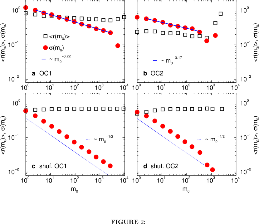
Figure 2: Average and standard deviation of the growth rate versus number of messages. a, Results for OC1. The average growth rate of messages conditional to $m_{0}$ is almost constant and the standard deviation decays with an exponent $\beta_{\rm OC1}=0.22\pm 0.01$. b, Results for OC2. The standard deviation conditional to $m_{0}$ decays with an exponent $\beta_{\rm OC2}=0.17\pm 0.03$. c, Results for OC1, when the messages are shuffled, displaying $\beta_{\rm rnd}=1/2$. d, Results for OC2, when the messages are shuffled. In all cases $t_{0}$ corresponds to half of the period of data acquisition and $t_{1}$ to the end, which we found to provide optimal statistics (see SI Fig. 1).

In Fig. 2a,b we show the results of $\langle r(m_{0})\rangle$ and $\sigma(m_{0})$ versus $m_{0}$ for both online communities. We find that the conditional average growth rate is fairly independent of $m_{0}$. On the other hand, the standard deviation decreases as a power-law of the form:

$$\sigma(m_{0})\sim m_{0}^{-\beta}\,.$$ (2)

We obtain by least square fitting the exponents $\beta_{\rm OC1}=0.22\pm 0.01$ for OC1 and $\beta_{\rm OC2}=0.17\pm 0.03$ for OC2 (the values deviate slightly for large $m_{0}$ due to low statistics). Although the web-sites are used by different member populations, the power-law and the obtained exponents are quite similar. The exponents are also close to those reported for growth in economic systems such as firms and countries ($0.15-0.18$, StanleyABHLMSS1996 ), research and development expenditures at universities ($0.25$, PlerouAGMS1999 ), scientific output ($0.28-0.4$, MatiaALMS2005 ), and city population growth ($0.19-0.27$, RozenfeldRABSM2008 ). The approximate agreement between the exponents obtained for very different systems (social or of human origin) can be considered as a generalization of Gibrat’s law, suggesting that the mechanisms behind the growth properties in different systems may originate in the human activity represented by Eq. (2).

Figures 2c and d depict the results when we randomize the data of OC1 and OC2, respectively (see Sec. IV for details of the randomization procedure), such that any temporal correlations are removed. The typical dynamics for such surrogate data set are shown in Fig. 1b (the brown curve) displaying a clear random pattern of small fluctuations in comparison with the original data of larger fluctuations (green curve). We find that the random signal displays a close to constant average growth rate $\langle r(m_{0})\rangle$ and that the fluctuations behave as in Eq. (2) but with an exponent $\beta_{\rm rnd}=1/2$ (Fig. 2c,d). The origin of this value has a simple explanation: If an isolated individual randomly flips an ideal coin with no memory of the previous attempt, then the fluctuations from the expected value of the fraction of obtained heads decay as a square-root of the number of throws, implying $\beta_{\rm rnd}=1/2$. In contrast to randomness, here we hypothesize that the origin of the generalized version of Gibrat’s law with $\beta<1/2$ in Eq. (2) is a non-trivial long-term correlation in communication activity. These correlations possibly arise from internal and external stimuli from other members transmitted through the highly connected network of individuals, an effect that is absent in the randomized data. The exponent value of $\beta\approx 0.2$ for OC1 and OC2 implies that the fluctuations of very active members are smaller than the ones of less active members, but they are significantly larger compared to the random case (compare Fig. 2a,b with Fig. 2c,d).

Long-term correlations

The exceptional quality of the data (more than 10 million messages spanning several effective decades of magnitude in terms of both activity and time) allows to test the above hypothesis by investigating the presence of temporal correlations in the individuals’ activity. We aggregate the data to records of messages per day (an example is shown in Fig. 1c) to avoid the daily cycle in the activity and analyze the number of messages sent by individuals per day, $\mu(t)$, where $t$ denotes the day [$m(t)\equiv\sum_{t^{\prime}=1}^{t}\mu(t^{\prime})$, Figs. 1d-f show the color coded daily activity of three members in OC1]. For every member we obtain a record of a length of $63$ days (OC1) or $492$ days (OC2). We note that former studies reporting Eq. (2) such as StanleyABHLMSS1996 ; PlerouAGMS1999 ; MatiaALMS2005 ; RozenfeldRABSM2008 typically were not based on data with temporal resolution as we use it here, and therefore were not able to investigate its origin in terms of temporal correlations.

We quantify the temporal correlations in the members’ activity by mapping the problem to a one-dimensional random walk. The quantity $Y(t)\equiv\sum_{t^{\prime}=1}^{t}\left(\mu(t^{\prime})-\langle\mu(t)\rangle\right)$, where $\langle\mu(t)\rangle$ is the average of the corresponding record $\mu(t)$, represents the position of the random walker that performs an up or down step given by $\mu(t^{\prime})-\langle\mu(t)\rangle$ at time step $t^{\prime}$. The correlations after $\Delta t$ steps are reflected in the behavior of the root-mean-square displacement $F(\Delta t)\equiv\sqrt{\langle\left[Y(t+\Delta t)-Y(t)\right]^{2}\rangle}$ Feder1988 , where $\langle\cdot\rangle$ is the average over $t$ and members. If the activity $\mu(t)$ is uncorrelated or short-term correlated, then one obtains $F(\Delta t)\sim(\Delta t)^{1/2}$, Fick’s law of diffusion, after some cross-over time. In the case of long-term correlations, the result is a power-law increase

$$F(\Delta t)\sim(\Delta t)^{H}\,,$$ (3)

where $H>1/2$ is the fluctuation exponent (also known as Hurst exponent Feder1988 ). In statistical physics, long-term correlation or persistence is also referred to as long-term “memory”. Since, in general, the records might be affected by trends, we use the standard Detrended Fluctuation Analysis (DFA) PengBHSSG94 to calculate $H$ (see SI Sec. III for a detailed description).

The results for OC1 are shown in Figs. 3a,b, where we calculate Eq. (3) by separating the members in groups with different total number of messages sent by the members, $M$. We find that $F(\Delta t)$ asymptotically follows a power-law with $H\approx 1/2$ for the less active members who sent less than $10$ messages in the entire period ($M<10$). The dynamics of the more active members display clear long-term correlations. We find that the fluctuation exponent increases to $H\approx 0.75$ for members with $M>10^{3}$ (see Fig. 3b). The smaller value of $H$ for less active members could be due to the small amount of information that these members provide in the available time of data acquisition. When we shuffle the data to remove any temporal correlations, we obtain the random exponent $H_{\rm rnd}=1/2$ (as seen in Fig. 3b), confirming that the correlations in the data are due to temporal structure.

The dynamics of the message activity in OC2 is similar to OC1 (see Fig. 3c). On large time scales we measure the fluctuation exponent increasing from $H\approx 1/2$ to $H\approx 0.9$ with increasing $M$ (the exponents for very active members are based on poor statistics and therefore carry large error bars). Analogous to the results obtained for OC1, there are no correlations in the shuffled records ($H_{\rm rnd}=1/2$ in Fig. 3d). The fact that $H>1/2$ means that a sudden burst in activity of a member persists on times scales ranging from days to years. The distribution of activity is self-similar over time. Similar correlation results have been found in traded values of stocks and email data EislerBK2008 .

Relation between $\beta$ and $H$

Next, we elaborate the mathematical framework that relates the growth process Eq. (2) to the long-term correlations, Eq. (3). To relate the exponent from Eq. (2), $\beta$, to the temporal correlation exponent $\gamma$, from Eq. (4), and therefore to $H$, one can first rewrite Eq. (1) as:

$$r = \ln\frac{m_{1}}{m_{0}}=\ln\frac{m_{0}+\Delta m}{m_{0}}\quad\textrm{ with }\Delta m=m_{1}-m_{0}$$

$$= \ln\left(\frac{\Delta m}{m_{0}}+1\right)\approx\frac{\Delta m}{m_{0}}\quad\textrm{ for small }\frac{\Delta m}{m_{0}}.$$

Next, the total increment of messages $\Delta m$ is expressed in terms of smaller increments $\mu(t)$, such as messages per day:

$$\Delta m=\sum_{t=t_{0}+1}^{t_{0}+\Delta t}\mu(t)\,,$$

which is (assuming stationarity) statistically equivalent to $\Delta m=\sum_{t=1}^{\Delta t}\mu(t)\,,$ and one can write $r\approx\frac{1}{m_{0}}\sum_{t=1}^{\Delta t}\mu(t)$ for the growth rate. The conditional average growth is then

$$\langle r(m_{0})\rangle = \langle\frac{1}{m_{0}}\sum_{t=1}^{\Delta t}\mu(t)\rangle\approx\frac{1}{m_{0}}\sum_{t=1}^{\Delta t}\langle\mu(t)\rangle\,.$$

Then, the conditional standard deviation $\sigma(m_{0})=\sqrt{\langle[r(m_{0})-\langle r(m_{0})\rangle]^{2}\rangle}\,,$ can be written in terms of the auto-correlation function as follows:

$$r(m_{0})-\langle r(m_{0})\rangle = \frac{1}{m_{0}}\left(\sum_{t=1}^{\Delta t}\mu(t)-\sum_{t=1}^{\Delta t}\langle\mu(t)\rangle\right)$$

$$\left[r(m_{0})-\langle r(m_{0})\rangle\right]^{2} = \frac{1}{m_{0}^{2}}\left(\sum_{t=1}^{\Delta t}\left(\mu(t)-\langle\mu(t)\rangle\right)\right)^{2}$$

$$\langle\left[r(m_{0})-\langle r(m_{0})\rangle\right]^{2}\rangle \approx \frac{1}{m_{0}^{2}}\sum_{i}^{\Delta t}\sum_{j}^{\Delta t}\sigma^{2}_{\mu}C(j-i)\,,$$

where $C(\Delta t)=\frac{1}{\sigma^{2}_{\mu}}\langle\left[\mu(t)-\langle\mu(t)\rangle\right]\left[\mu(t+\Delta t)-\langle\mu(t)\rangle\right]\rangle$ is the auto-correlation function of $\mu(t)$ and $\sigma_{\mu}$ is the standard deviation of $\mu(t)$. The auto-correlation function $C(\Delta t)$ measures the interdependencies between the values of the record $\mu(t)$. For uncorrelated values, $C(\Delta t)$ is zero for $\Delta t>0$, because on average positive and negative products of the record will cancel out each other. In the case of short-term correlations, $C(\Delta t)$ has a characteristic decay time, $\Delta t_{\times}$. A prominent example is the exponential decay $C(\Delta t)\sim\exp(-\Delta t/\Delta t_{\times})$. Long-term correlations are described by a slower decay namely a power-law,

$$C(\Delta t)\sim(\Delta t)^{-\gamma}\,,$$ (4)

with the correlation exponent $0<\gamma<1$ which is related to the fluctuation exponent $H$ from Eq. (3) by $\gamma=2-2H$ Feder1988 . We note that $\gamma=1$ (or $\gamma>1$) corresponds to an uncorrelated record with $H=1/2$. A key-property of long-term correlations is a pronounced mountain-valley structure in the records Feder1988 . Statistically, large values of $\mu(t)$ are likely to be followed by large values and small values by small ones. Ideally, this holds on all time scales, which means a sequence in daily, weekly or monthly resolution is correlated in the same way as the original sequence.

Assuming long-term correlations asymptotically decaying as in Eq. (4), we approximate the double sum with integrals and obtain:

$$\langle\left[r(m_{0})-\langle r(m_{0})\rangle\right]^{2}\rangle \approx \frac{1}{m_{0}^{2}}\sigma_{\mu}^{2}\int\!\!\!\int_{1}^{\Delta t}\!\!(j-i)^{-\gamma}{\rm d}j{\rm d}i\sim\frac{1}{m_{0}^{2}}\sigma_{\mu}^{2}\left(\Delta t\right)^{2-\gamma}\,.$$

In order to relate $\Delta t$ and $m_{0}$, one can use $\Delta t=x\,t_{0}\,,$ where $x$ is an arbitrary (small) constant, that simply states how large $\Delta t$ is compared to $t_{0}$, and $m_{0}\sim t_{0}\,,$ which states that the number of messages is proportional to time assuming stationary activity. Using these two arguments we obtain:

$$\langle\left[r(m_{0})-\langle r(m_{0})\rangle\right]^{2}\rangle \approx \frac{1}{m_{0}^{2}}\sigma_{\mu}^{2}\left(x\right)^{2-\gamma}\left(t_{0}\right)^{2-\gamma}\sim\sigma_{\mu}^{2}m_{0}^{-\gamma},$$

$$\sigma(m_{0}) \sim \sigma_{\mu}m_{0}^{-\gamma/2}\,.$$

Comparing with Eq. (2), we finally obtain $\beta=\gamma/2\,,$ and with $\gamma=2-2H$:

$$\beta=1-H\,.$$ (5)

Equation (5) is a scaling law formalizing the relation between growth and long-term correlations in the activity and is confirmed by our data. For OC1 we measured $\beta_{\rm OC1}\approx 0.22$ yielding $H_{\rm OC1}\approx 0.78$ from Eq. (5), which is in approximate agreement with the (maximum) exponent we obtained by direct measurements for OC1 ($H=0.75\pm 0.05$ from Fig. 3b). For OC2 we obtained $\beta_{\rm OC2}\approx 0.17$ and therefore $H_{\rm OC2}\approx 0.83$ through Eq. (5) which is not too far from the (maximum) exponent found by direct measurements for OC2 ($H=0.88\pm 0.03$). According to Eq. (5), the original Gibrat’s law ($\beta_{\rm G}=0$) corresponds to very strong long-term correlations with $H_{\rm G}=1$. This is the case when the activity on all time scales exhibits equally strong correlations. In contrast, $\beta_{\rm rnd}=1/2$ represents completely random activity $(H_{\rm rnd}=1/2)$, as obtained for the randomized data in Fig. 3b,d.

The mathematical framework relating long-term correlations quantified by $H$ and the growth fluctuations quantified by $\beta$ could be relevant to other complex systems. While the generalized version of Gibrat’s law has been reported for economic indicators displaying $\beta\approx 0.2$ StanleyABHLMSS1996 ; PlerouAGMS1999 ; MatiaALMS2005 , the origin of this scaling law is not clear and still being investigated. Our results suggest that the value of $\beta$ could be explained by the existence of long-term correlations in the activity of the corresponding system ranging from firms and markets to social and population dynamics. In turn, Eq. (5) establishes a missing link between studies of growth processes in economic or social systems StanleyABHLMSS1996 ; PlerouAGMS1999 ; MatiaALMS2005 and studies of long-term correlations such as in finance and the economy MantegnaS1999 , Ethernet traffic LelandTWW1994 , human brain LinkenkaerHansenNPI2001 or motor activity IvanovHHSS2007 . Our results foreshadow that systems involving other types of human interactions such as various Internet activities, communication via cell phones, trading activity, etc. may display similar growth and correlation properties as found here, offering the possibility of explaining their dynamics in terms of the long-term persistence of the individuals’ behavior.

Growth of the degree in the underlying social network

Communication among the members of a community represents a type of a social interaction that defines a network, whereas a message is sent either based on an existing relation between two members or establishing a new one. There is considerable interest in the origin of broad distributions of activity in social systems. Two paradigms have been invoked for various applications in social systems: the “rich-get-richer” idea used by Simon in 1955 SimonHA1955 and the models based on optimization strategies as proposed by Mandelbrot MandelbortB1953 . Regarding network models, the preferential attachment (PA) model has been introduced BarabasiA1999 to generate a type of stochastic scale-free networks with a power-law degree distribution in the network topology. Considering the social network of members linked when they exchange at least one message (that has not been sent before), we examine the dynamic of the number of outgoing links of each member [the out-degree $k(t)$] in analogy to Eqs. (2).

We start from the empty set of nodes consisting of all the members in the community and chronologically add a directed link between two members when a messages is sent. In analogy to the growth in the number of messages $m(t)$ of each member, we study the growth of the members’ out-degree $k(t)$, i.e. the number of links to others. We define the growth rate of every member as

$$r_{k}=\ln\frac{k_{1}}{k_{0}}\,,$$ (6)

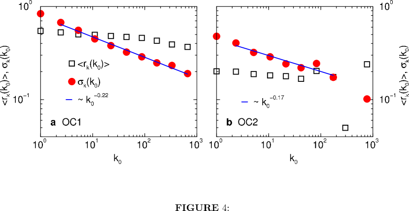
Figure 4: Mean out-degree growth rate and standard deviation versus initial out-degree. a, Results for OC1. The average growth of out-degree conditional to the out-degree at $t_{0}$ is almost constant. The standard deviation decays with an exponent $\beta_{k,{\rm OC1}}=0.22\pm 0.02$. b, Results for OC2. The standard deviation conditional to the out-degree at $t_{0}$ decays with an exponent $\beta_{k,{\rm OC2}}=0.17\pm 0.08$. The quantities are analogous to those of Fig. 2 except that here the growth rate of the out-degree $r_{k}$ is considered instead of the number of messages sent.

where $k_{0}\equiv k(t_{0})$ is the out-degree of a member at time $t_{0}$ and $k_{1}\equiv k(t_{1})$ is the out-degree at time $t_{1}$. Again, there is a growth rate for each member $j$, but for a better readability, we skip the index. In Fig. 4 we study $\langle r_{k}(k_{0})\rangle$, the average growth rate conditional to the initial out-degree $k_{0}$, and $\sigma_{k}(k_{0})$, the standard deviation of the growth rate conditional to the initial out-degree $k_{0}$ for OC1 and OC2. We obtain almost constant average growth $\langle r_{k}(k_{0})\rangle$ as a function of $k_{0}$ as in the study of messages.

The conditional standard deviation of the network-degree, $\sigma_{k}(k_{0})$, is shown in Fig. 4 for both social communities. We obtain a power-law relation analogous to Eq. (2):

$$\sigma_{k}(k_{0})\sim k_{0}^{-\beta_{k}}\,,$$ (7)

with fluctuation exponents very similar to those found for the number of messages, namely $\beta_{k,{\rm OC1}}=0.22\pm 0.02$ for OC1 and $\beta_{k,{\rm OC2}}=0.17\pm 0.08$ for OC2. This values are consistent with those we obtained for the activity of sending messages.

Next, we consider the preferential attachment model which has been introduced to generate scale-free networks BarabasiA1999 with power-law degree distribution $P(k)$ of the type investigated in the present study. Essentially, it consists of subsequently adding nodes to the network by linking them to existing nodes which are chosen randomly with a probability proportional to their degree. We consider the undirected network and study the degree growth properties using Eqs. (6) and (7) and calculate the conditional average growth rate $\langle r_{\rm PA}(k_{0})\rangle$ and the conditional standard deviation $\sigma_{\rm PA}(k_{0})$. The times $t_{0}$ and $t_{1}$ are defined by the number of nodes attached to the network. Figure 2 in the SI Sec. IV shows the results where an average degree $\langle k\rangle=20$; $50,000$ nodes in $t_{0}$, and $100,000$ nodes in $t_{1}$ were chosen. We find constant average growth rate that does not depend on the initial degree $k_{0}$. The conditional standard deviation is a function of $k_{0}$ and exhibits a power-law decay characterized by Eq. (7), respectively Eq. (2), with $\beta_{\rm PA}=1/2$. The value $\beta_{\rm PA}=1/2$ in Eq. (5) corresponds to $H=1/2$ indicating complete randomness. There is no memory in the system. Since each addition of a new node is completely independent from precedent ones, there cannot be temporal correlations in the activity of adding links. Therefore, purely preferential attachment type of growth is not sufficient to describe the social network dynamics found in the present study and further temporal correlations have to be incorporated according to Eq. (3).

For the PA model it has been shown that the degree of each node grows in time as $k(t)\sim\left(\frac{t}{t^{*}}\right)^{b}$, where $t^{*}$ is the time when the corresponding node was introduced to the system and $b=1/2$ is the dynamics exponent in growing network models AlbertB2002 . Accordingly, the growth rate is given by $r_{\rm PA}=b\ln\frac{t_{1}}{t_{0}}$, which is constant independent of $k_{0}$, in accordance with our numerical findings. Furthermore, in SI Sec. IV we obtain analytically the exponent $\beta_{\rm PA}=1/2$ confirming the numerical results, as well. Interestingly, an extension of the standard PA model has been proposed BianconiB2001 that takes into account different fitnesses of the nodes to acquiring links involving a distribution of $b$-exponents and therefore a distribution of growth rates. This model opens the possibility to relate the distribution of fitness values to the fluctuations in the growth rates, a point that requires further investigation.

III Discussion

From a statistical physics point of view, the finding of long-term correlations opens the question of the origin of such a persistence pattern in the communication. At this point we speculate on two possible scenarios, which require further studies. The question is whether the finding of an exponent $H>0.5$ is due to a power-law (Levy type) distribution ShlesingerFK1987 ; BuldyrevGHPSS1993 in the time interval between two messages of the same person or just from pure correlations or long-term memory in the activity of people. In the first scenario, the intervals between the messages follow a power-law BarabasiAL2005 ; GersteinM1964 . Accordingly, the activity pattern comprises many short intervals and few long ones, implying persistent epochs of small and large activity. This fractal-like activity leads to long-term correlations with $H>1/2$ (see the analogous problem of the origin of long-term correlations in DNA sequences as discussed in BuldyrevGHPSS1993 ). This scenario implies a direct link between the correlations and the distribution of inter-event intervals which can be obtained analytically. In the second scenario, the intervals between the messages do not follow a Levy type distribution, but the value of the time intervals are not independent of each other, again representing long-term persistence. For example, the distribution of inter-event times could be stretched exponential (see recent work on the study of extreme events of climatological records exhibiting long-term correlations BundeEKH2005 ). Thus, deciding between these two possible scenarios for the origin of correlations in activity requires an extended analysis of inter-event intervals as well as correlations to determine whether the behavior is Levy-like or pure memory like. A careful statistical analysis is needed which will be the focus of future research.

To some extent, the human nature of persistent interactions enables the prediction of the actants’ activity. Our finding implies that traditional mean-field approximations based on the assumption that the particular type of human activity under study can be treated as a large number of independent random events (Poisson statistics) may result in faulty predictions. On the contrary, from the growth properties found here, one can estimate the probability for members of certain activity level to send more than a given number of messages in the future. This result may help to improve the proper allocation of resources in communication-based systems ranging from economic markets to political systems. As a byproduct, our finding that the activity of sending messages exhibits long-term persistence suggests the existence of an underlying long-term correlated process. This can be understood as an unknown individual state driven by various internal and external stimuli HedstroemP2005 ; KentsisA2006 providing the probability to send messages. In addition, the memory in activity found here could be the origin of the long-term persistence found in other records representing a superposition of the individuals’ behavior, such as the Ethernet traffic LelandTWW1994 , highway traffic, stock markets, and so forth.

IV Materials and Methods

Calculations of $\langle r(m_{0})\rangle$, $\sigma(m_{0})$ and optimal times $t_{0}$ and $t_{1}$

The average growth rate, $\langle r(m_{0})\rangle$, and the standard deviation, $\sigma(m_{0})=\sqrt{\langle r(m_{0})^{2}\rangle-\langle r(m_{0})\rangle^{2}}$, are defined as follows. Calling $P(r|m_{0})$ the conditional probability density of finding a member with growth rate $r(m_{0})$ with the condition of initial number of messages $m_{0}$, then we obtain:

$$\langle r(m_{0})\rangle=\int\!\!rP(r|m_{0})\,{\rm d}r\,,$$ (8)

and

$$\langle r(m_{0})^{2}\rangle=\int\!\!r^{2}P(r|m_{0})\,{\rm d}r\,.$$ (9)

In order to calculate the growth rate Eq. (1), one has to choose the times $t_{0}$ and $t_{1}$ in the period of data acquisition $T$. Naturally, it is best to use all data in order to have optimal statistics. Accordingly, $t_{1}$ is chosen best at the end of the available data ($t_{1}=T$). We argue that if the choice of $t_{0}$ is too small, then $m(t_{0})$ is zero for many members (those that send their messages later), which are then rejected in the calculation because of the division in Eq. (1). Conversely, if $t_{0}$ is chosen too large, then there is not enough time to observe the member’s activity and $r=0$ will occur frequently, indicating no change (members have sent their messages before). Thus, there must be an optimal time in between. In SI Sec. II, Fig. 1, we plot, as a function of $t_{0}$, the number of members with at least one message at $t_{0}$ [$m_{0}>0$] and further exhibit at least some activity until $t_{1}=T$ [$m_{1}-m_{0}>0$]. For both online communities we find an optimal $t_{0}$ in the middle of the period of observation $t_{0}=T/2$, a value that is used for the analysis in the main text.

Shuffling of the message data

The raw data comprises one entry for each message consisting of the time when the message is sent, the sender identifier and the receiver identifier. For example:

time	sender	receiver
1	a	b
2	a	c
4	b	a
6	c	d
7	a	b
…

This means, at $t=1$ member a sends a message to member b, at $t=2$ member a sends a message to member c, and so on.

The randomized surrogate data set is created by randomly swapping the instants (time) at which the messages are sent between two events chosen at random. Thus, each message entry randomly obtains the time of another one. This means the total number of messages is preserved and the associations between them get shuffled. Temporal correlations are destroyed, but the set of instants at which the messages are sent remains unchanged. For instance, swapping events at $t=1$ and $t=6$ results in: $t=1$, c$\,\rightarrow\,$d, and $t=6$, a$\,\rightarrow\,$b.

Acknowledgments

We thank NSF-SES-0624116 for financial support and C. Briscoe, L. K. Gallos and H. D. Rozenfeld for discussions. F. L. acknowledges financial support from The Swedish Bank Tercentenary Foundation.

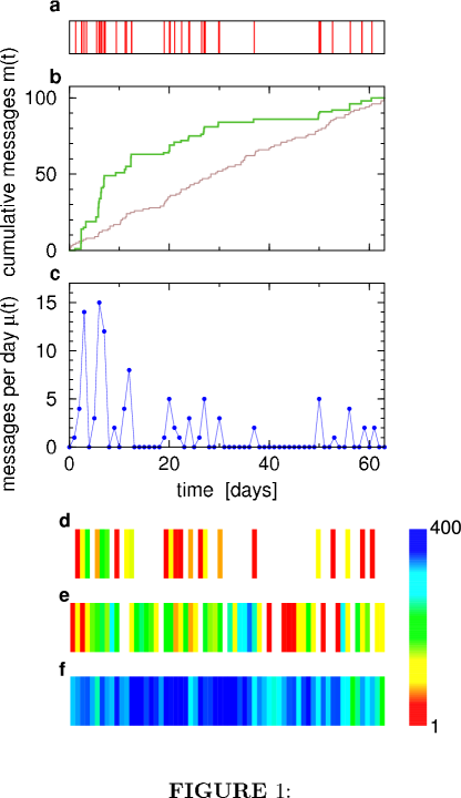
Figure 1: A typical example of an individuals’ message activity. a, Instants at which messages were sent by a member belonging to OC1. b, Cumulative number of messages $m(t)$ (green) and the same but with the messages placed at random (brown). c, Sequence of number of messages sent per day, $\mu(t)$, for the same individual. d,e,f, Color coded sequences $\mu(t)$ for members sending $M=100$; 1,000; or 10,000 messages overall, respectively. The color is proportional to the logarithm of the number of messages per day (red: $1$ message, blue: $400$ messages, white for no message).

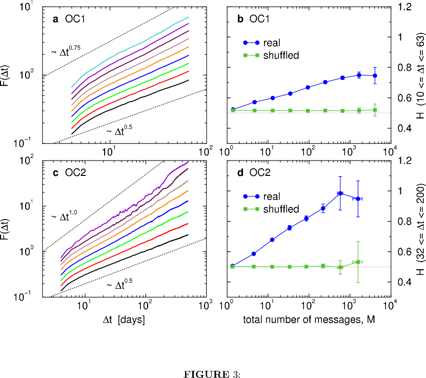
Figure 3: Long-term correlations in the message activity of OC1 (a and b) and OC2 (c and d). a, DFA fluctuation functions averaged conditional to $M$, the total number of messages sent by each member (black: 1-2, red: 3-7, green: 8-20, blue: 21-54, orange: 55-148, brown: 149-403, maroon: 404-1096, violet: 1097-2980, turquoise: 2981-8103). The dotted lines serve as guides, the one in the bottom corresponds to the uncorrelated case, while the one in the top corresponds to the exponent $0.75$. b, Fluctuation exponent $H$ measured from panel a on the scales $10\textrm{ days}\leq\Delta t\leq 63\textrm{ days}$ as a function of the total number of messages sent, $M$, for real (blue) and individually shuffled (green) records. c, DFA fluctuation functions averaged conditional to $M$ [colors as in (A)]. The dotted lines correspond to the uncorrelated case (bottom) and to the exponent $1$ (top). d, Fluctuation exponents obtained from panel c on the scales $32\textrm{ days}\leq\Delta t\leq 200\textrm{ days}$ as a function of the total number of messages sent, $M$. Due to weak statistics causing large error bars we do not consider the last two values for $M>500$ as reliable. For clarity the fluctuation functions in panels a and c are shifted vertically.

SUPPORTING INFORMATION (SI)

I Notation

1. Member $j$ sends his/her $n$th message at time $t_{j}(n)$, where $1\leq n\leq M_{j}$ and $M_{j}$ is the total number of messages sent by $j$ in the time of data acquisition $T$. The sequence of counts defined as the number of messages in the period $\delta t$, is given by

   $$\mu_{j}^{\delta t}(t)=\sum_{n,t_{j}(n)\in[t,t+\delta t]}a_{j}(n)\,,$$ (10)

   where $a_{j}(n)=1$. In addition, the periods are non-overlapping, $t=i\delta t$ with integer $i$, and therefore $1\leq t_{j}(n)\leq T$. In the case of daily resolution $\delta t=1$ day.

2. The cumulative number of messages that a member sends until time $t$ is:

   $$m_{j}^{\delta t}(t)=\sum_{t^{\prime}=1}^{t}\mu_{j}^{\delta t}(t^{\prime})\,.$$ (11)

   In particular, $m_{j}(1)=\mu_{j}(1)$ and $m_{j}(T)=M_{j}$.

3. The displacement of the random walk is the cumulative sum of the normalized $\mu_{j}^{\delta t}(t)$:

   $$Y_{j}^{\delta t}(t)=\sum_{t^{\prime}=1}^{t}(\mu_{j}^{\delta t}(t^{\prime})-\langle\mu_{j}^{\delta t}(t)\rangle)\,,$$ (12)

   where $\langle\mu_{j}^{\delta t}(t)\rangle$ is the average of $\mu_{j}^{\delta t}(t)$ in time $t$. The root-mean-square displacement after $\Delta t$ is defined as

   $$F_{j}^{\delta t}(\Delta t)=\sqrt{\langle[Y_{j}^{\delta t}(t+\Delta t)-Y_{j}^{\delta t}(t)]^{2}\rangle}_{t}\,,$$ (13)

   where the average is performed over the time $t$. Additionally, we perform an average over members $j$ with activity level $M$ and define

   $$(F^{\delta t}(\Delta t))^{2}_{M}=\langle(F_{j}^{\delta t})^{2}|M\rangle_{j}\,.$$ (14)

4. For simplicity, in the main text we skip the index $j$ as well as $\delta t$ and write $\mu(t)$, $m(t)$, $Y(t)$, as well as $F(\Delta t)$.

5. To investigate the growth in the number of messages we use the quantities $r=\ln\frac{m_{1}}{m_{0}}$, $\langle r(m_{0})\rangle$, $\sigma(m_{0})$ and the exponents $\beta_{\rm OC1}$, $\beta_{\rm OC2}$, $\beta_{\rm G}$, $\beta_{\rm rnd}$.

6. To investigate the growth of the degree we use the quantities $r_{k}=\ln\frac{k_{1}}{k_{0}}$, $\langle r_{k}(k_{0})\rangle$, $\sigma_{k}(k_{0})$ and the exponents $\beta_{k,{\rm OC1}}$; $\beta_{k,{\rm OC2}}$.

7. For the growth of the degree in the preferential attachment model we use the quantities $r_{\rm PA}=\ln\frac{k_{1}}{k_{0}}$, $\langle r_{\rm PA}(k_{0})\rangle$, $\sigma_{\rm PA}(k_{0})$ and the exponent $\beta_{\rm PA}$.

II Optimal times $t_{0}$ and $t_{1}$

Figure  5 displays the optimal times $t_{0}$ and $t_{1}$ to calculate the growth rates for OC1 (panel a) and OC2 (panel b).

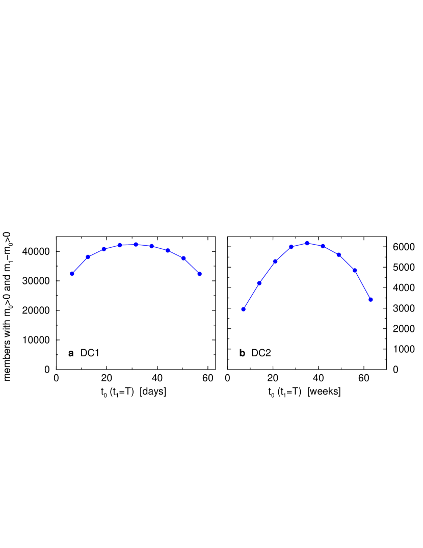
Figure 5: Optimal times $t_{0}$ and $t_{1}$. The panels show for a, OC1, and b, OC2, the number of members with both, $m_{0}>0$ and $m_{1}-m_{0}>0$. While $t_{1}$ obviously is optimal at the end of the period, $t_{0}$ is varied to find the value for which the number of members – with at least one message until $t_{0}$ and at least one new message between $t_{0}$ and $t_{1}$ – is maximal.

III Details on the quantification of long-term correlations using Detrended Fluctuation Analysis

Statistical dependencies between the values of a record $\mu(t)$ with $t=1,\dots,T$ can be characterized by the auto-correlation function

$$C(\Delta t)=\frac{1}{\sigma_{\mu}^{2}(T-\Delta t)}\sum_{t=1}^{T-\Delta t}\left[\mu(t)-\langle\mu(t)\rangle\right]\left[\mu(t+\Delta t)-\langle\mu(t)\rangle\right]\,,$$ (15)

where $T$ is the length of the record $\mu(t)$, $\langle\mu(t)\rangle$ its average, and $\sigma_{\mu}$ its standard deviation. For uncorrelated values of $\mu(t)$, $C(\Delta t)$ is zero for $\Delta t>0$, because on average positive and negative products will cancel each other out. In the case of short-term correlations $C(\Delta t)$ has a characteristic decay time $\Delta t_{\times}$. A prominent example is the exponential decay $C(\Delta t)\sim\exp(-\Delta t/\Delta t_{\times})$. Long-term correlations are described by a slower decay, e.g. diverging $\Delta t_{\times}$, namely a power-law,

$$C(\Delta t)\sim(\Delta t)^{-\gamma}\,,$$ (16)

with the correlation exponent $0<\gamma<1$.

Detrended Fluctuation Analysis (DFA) is a well studied method to quantify long-term correlations in the presence of non-stationarities PengBHSSG94 . The analysis of a considered record $\mu(t)$ of length $T$ consists of 5 steps:

1. Calculate the cumulative sum, the so-called profile:

   $$Y(t)=\sum_{t^{\prime}=1}^{t}\left(\mu(t^{\prime})-\langle\mu(t)\rangle\right)\,.$$ (17)

2. Separate the profile $Y(t)$ into $T_{\Delta t}={\rm int}\frac{T}{\Delta t}$ segments of length $\Delta t$. Often, the length of the record is not a multiple of $\Delta t$. In order not to disregard information, the segmentation procedure is repeated starting from the end of the record and one obtains $2T_{\Delta t}$ segments.

3. Locally detrend each segment $\nu$ by determining best polynomial fits $p^{(n)}_{\nu}(t)$ of order $n$ and subsequently subtract it from the profile:

   $$Y_{\Delta t}(t)=Y(t)-p^{(n)}_{\nu}(t)\,.$$ (18)

4. Calculate for each segment the variance (squared residuals) of the detrended $Y_{\Delta t}(t)$

   $$F_{\Delta t}^{2}(\nu)=\frac{1}{\Delta t}\sum_{j=1}^{\Delta t}\left(Y_{\Delta t}^{2}\left[(\nu-1)\Delta t+j\right]\right)$$ (19)

   by averaging over all values in the corresponding $\nu$th segment.

5. The DFA fluctuation function is given by the square-root of the average over all segments:

   $$F(\Delta t)=\left[\frac{1}{2T_{\Delta t}}\sum_{\nu=1}^{2T_{\Delta t}}F_{\Delta t}^{2}(\nu)\right]^{1/2}\,.$$ (20)

   The averaging of $F_{\Delta t}^{2}(\nu)$ is additionally performed over members of similar activity level $M$.

If the record $\mu(t)$ is long-term correlated according to a power-law decaying auto-correlation function, Eq. (16), then $F(\Delta t)$ increases for large scales $\Delta t$ also as a power-law:

$$F(\Delta t)\sim(\Delta t)^{H}\,,$$ (21)

where the fluctuation exponent $H$ is analogous to the well-known Hurst exponent Feder1988 . The exponents are related via

$$H=1-\gamma/2\enspace,\qquad\gamma=2-2H\,.$$ (22)

When $\gamma=1$ then $H_{\rm rnd}=1/2$, that is the case of uncorrelated dynamics. If the correlations decay faster than $\gamma>1$ then the random exponent $H_{\rm rnd}=1/2$ is still recovered. Long-term correlations imply $0<\gamma<1$ and $1/2<H<1$. In practice, one plots $F(\Delta t)$ versus $\Delta t$ in double-logarithmic representation, determines the exponent $H$ on large scales and quantifies the correlation exponent $\gamma$. The order of the polynomials $p^{(n)}_{\nu}$ determines the detrending technique which is named DFA$n$, DFA$0$ for constant detrend, DFA$1$ for linear, DFA$2$ for parabolic, etc.

The subtraction of the average in Eq. (17) is only necessary for DFA$0$. By definition the corresponding fluctuation function is only given for $\Delta t\geq n+2$. The detrending order determines the capability of detrending. Since the local trends are subtracted from the profile, only trends of order $n-1$ are subtracted from the original record $\mu(t)$. Throughout the paper we show the results using DFA$2$ which we found to be sufficient in terms of detrending.

Since the fluctuation functions $F(\Delta t)$ for single users are very noisy, it is useful to average fluctuation functions among various members. Thus, we first group the members in logarithmic bins according to their activity level, the total number of messages $M$ sent. Namely, we group all members that send 1-2, 3-7, 8-20, …messages in the period of data acquisition by using bins determined by $b={\rm int}\left(\ln M\right)$. Next we average the fluctuation function among all members from each group $b$ and obtain for every activity level of the members one DFA fluctuation function. The error bars in Fig. 3a,c of the main text were obtained by subdividing each group and determining the standard deviations of the fluctuation exponents from different groups of the same activity level.

IV Growth in the degree

Figure 6 shows the results of the average growth rates and fluctuations of the growth rates as a function of the initial degree for the preferential attachment model BarabasiA1999 . We find a constant average growth rate and a standard deviation decreasing as a power law with exponent $\beta_{\rm PA}=1/2$ in Eq. (7) in the main text.

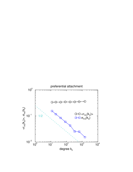
Figure 6: Growth properties of the preferential attachment model BarabasiA1999 discussed in the main text. We plot the average (black circles) and standard deviation (blue squares) of the growth rate $r_{\rm PA}$ conditional to $k_{0}$, the degree of the corresponding nodes at the first stage.

The PA network model has been described analytically. In particular, it has been shown that each nodes’ degree increases as

$$k(t)\sim\left(\frac{t}{t^{*}}\right)^{b}\,,$$ (23)

where $t^{*}$ is the time when the corresponding node was introduced to the system and $b$ is the dynamics exponent in growing network models ($b=1/2$ for the standard PA) AlbertB2002 . Accordingly, here the growth rate, Eq. (6) in the main text, is $r_{\rm PA}=\frac{1}{2}\ln\frac{t_{1}}{t_{0}}$, which we also find in Fig. 6.

To obtain $\sigma_{\rm PA}(k_{0})$ one can use analogous considerations as for $\sigma(m_{0})$ in the main text. Due to Eq. (6) in the main text, here we have

$$r_{\rm PA}\approx\frac{1}{k_{0}}\sum_{t=1}^{\Delta t}\kappa(t)\,,$$ (24)

where $\kappa(t)$ are small increments analogous to $\mu(t)$, whereas Eq. (23) implies

$$\kappa(t)\sim(\Delta t)^{-1/2}\,.$$ (25)

As before, the conditional standard deviation of the growth rate is

$$\langle\left[r_{\rm PA}(k_{0})-\langle r_{\rm PA}(k_{0})\rangle\right]^{2}\rangle\approx\frac{1}{k_{0}^{2}}\sum_{i}^{\Delta t}\sum_{j}^{\Delta t}\sigma^{2}_{\kappa}C(j-i)\,.$$ (26)

In the uncorrelated case $C(j-i)=\delta_{ij}$, the double sum can be reduced to a single one:

$$\sigma^{2}_{\rm PA}(k_{0})=\frac{1}{k_{0}^{2}}\sum_{i}^{\Delta t}\sigma^{2}_{\kappa}(i)\,.$$ (27)

As shown below, $\sigma_{\kappa}(i)\sim i^{-1/4}$, and integration leads to

$$\sigma^{2}_{\rm PA}(k_{0}) \sim \frac{1}{k_{0}^{2}}\int^{\Delta t}\!\!\!i^{-1/2}{\rm d}i$$ (28)

$$\sim \frac{1}{k_{0}^{2}}(\Delta t)^{1/2}\,.$$ (29)

Eliminating $\Delta t$ using $k\sim t^{-1/2}$, Eq. (23), one obtains

$$\sigma_{\rm PA}(k_{0})\sim k_{0}^{-1/2}\,.$$ (30)

That is, we obtain $\beta_{\rm PA}=1/2$ as found numerically.

Remains to show $\sigma_{\kappa}(t)\sim t^{-1/4}$. We assume new links are set according to a Poisson process, whereas every new link of a node represents an event. The intervals between these events (asymptotically) follow an exponential distribution $p(\tau)=\lambda{\rm e}^{-\lambda\tau}$. Accordingly, $\kappa(t)$ is a sequence of zeros and only one when a new link is set to the corresponding node. The standard deviation of this sequence is

$$\sigma_{\kappa}\sim\lambda^{1/2}\,.$$ (31)

Due to Eq. (23) the rate parameter decreases like

$$\lambda(t)\sim t^{-1/2}\,.$$ (32)

Accordingly,

$$\sigma_{\kappa}(t)\sim t^{-1/4}\,.$$ (33)

In order to extend the standard PA model, a fitness model has been introduced BianconiB2001 taking into account different fitnesses of the nodes of acquiring links and therefore involving a distribution of $b$-exponents. The spread of growth rates $r$ could be related to the distribution of fitness. On the other hand, the growth according to Eq. (23) is superimposed with random fluctuations that we characterize with the exponent $\beta$.

References

- (1) Merton RK (1936) The Unanticipated Consequences of Purposive Social Action. Am Sociol Rev 1:894–904.
- (2) Weber M (1968) Economy and Society, Vol.1. (University of California Press, Berkley).
- (3) Giddens A (1993) New Rules of Sociological Method. (Stanford University Press, Stanford).
- (4) Durkheim E (1997) Suicide, reprint from 1897. (The Free Press, New York).
- (5) Pareto V (1896) Cours d’Economie Politique. (Droz, Geneva).
- (6) Zipf G (1932) Selective Studies and the Principle of Relative Frequency in Language. (Harvard University Press, Cambridge, MA).
- (7) Gibrat R (1931) Les inégalités économiques. (Libraire du Recueil Sierey, Paris).
- (8) Sutton J (1997) Gibrat’s Legacy. J Econ Lit 35:40–59.
- (9) Gabaix X (1999) Zipf’s law for cities: An explanation. Q J Econ 114:739–767.
- (10) Holme P, Edling CR, Liljeros F (2004) Structure and time evolution of an Internet dating community. Soc Networks 26:155–174.
- (11) Paxson V, Floyd S (1995) Wide area traffic: the failure of Poisson modeling. IEEE/ACM Trans Networking 3:226–244.
- (12) Dewes C, Wichmann A, Feldman A (2003) Proc. 2003 ACM SIGCOMM Conf. Internet Measurement (IMC-03). (ACM Press, New York).
- (13) Barabási A-L (2005) The origin of bursts and heavy tails in human dynamics. Nature 435:207–211.
- (14) Oliveira JG, Barabási A-L (2005) Darwin and Einstein correspondence patterns. Nature 437:1251.
- (15) Zhou T, Kiet HAT, Kim BJ, Wang B-H, Holme P (2008) Role of activity in human dynamics. Europhys Lett 82:28002.
- (16) Stanley MHR, et al. (1996) Scaling behaviour in the growth of companies. Nature 379:804–806.
- (17) Plerou V, Amaral LAN, Gopikrishnan P, Meyer M, Stanley HE (1999) Similarities between the growth dynamics of university research and of competitive economic activities. Nature 400:433–437.
- (18) Matia K, Amaral LAN, Luwel M, Moed HF, Stanley HE (2005) Scaling Phenomena in the Growth Dynamics of Scientific Output. J Am Soc Inf Sci Tec 56:893–902.
- (19) Rozenfeld HD, et al. (2008) Laws of Population Growth. Proc Nat Acad Sci USA 105:18702–18707.
- (20) Feder J (1988) Fractals, Physics of Solids and Liquids. (Plenum Press, New York).
- (21) Peng C-K, et al. (1994) Mosaic organization of DNA nucleotides. Phys Rev E 49:1685–1689.
- (22) Eisler Z, Bartos I, Kertész J (2008) Fluctuation scaling in complex systems: Taylor’s law and beyond. Adv Phys 57:89–142.
- (23) Mantegna RN, Stanley HE (1999) An Introduction to Econophysics: Correlations and Complexity in Finance. (Cambridge University Press, Cambridge).
- (24) Leland WE, Taqqu MS, Willinger W, Wilson DV (1994) On the Self-Similar Nature of Ethernet Traffic (Extended Version) IEEE/ACM Trans Networking 2:1–15.
- (25) Linkenkaer-Hansen K, Nikouline VV, Palva JM, Ilmoniemi RJ (2001) Long-range temporal correlations and scaling behavior in human brain oscillations. J Neurosci 21:1370–1377.
- (26) Ivanov PC, Hu K, Hilton MF, Shea SA, Stanley HE (2007) Endogenous circadian rhythm in human motor activity uncoupled from circadian influences on cardiac dynamics. Proc Nat Acad Sci USA 104:20702–20707.
- (27) Simon HA (1955) On a Class of Skew Distribution Functions. Biometrika 42:425–440.
- (28) Mandelbrot B (1953) An informational theory of the statistical structure of language, ed. Jackson, W. (Butterworth, London), pp. 486–504.
- (29) Barabási A-L, Albert R (1999) Emergence of scaling in random networks. Science 286:509–512.
- (30) Albert R, Barabási A-L (2002) Statistical mechanics of complex networks. Rev Mod Phys 74:47–97.
- (31) Bianconi G, Barabási, A-L (2001) Competition and multiscaling in evolving networks. Europhys Lett 54:436-442.
- (32) Shlesinger MF, West BJ, Klafter J (1987) Lévy dynamics of enhanced diffusion: Application to turbulence. Phys Rev Lett 58:1100–1103.
- (33) Buldyrev SV, Goldberger AL, Havlin S, Peng C-K, Simons M, Stanley HE (1993) Generalized Lévy-walk model for DNA nucleotide sequences. Phys Rev E 47:4514–4523.
- (34) Gerstein GL, Mandelbrot B (1964) Random walk models for spike activity of single neuron. Biophys J 4:41–68.
- (35) Bunde A, Eichner JF, Kantelhardt JW, Havlin S (2005) Long-Term Memory: A Natural Mechanism for the Clustering of Extreme Events and Anomalous Residual Times in Climate Records. Phys Rev Lett 94:048701.
- (36) Hedström P (2005) Dissecting the Social: On the Principles of Analytical Sociology. (Cambridge University Press, Cambridge).
- (37) Kentsis A (2006) Mechanisms and models of human dynamics. Nature 441:E5–E6.