Spin-charge decoupling and the photoemission line-shape in one dimensional insulators

Abstract

The recent advances in angle resolved photoemission techniques allowed the unambiguous experimental confirmation of spin charge decoupling in quasi one dimensional (1D) Mott insulators. This opportunity stimulates a quantitative analysis of the spectral function $A(k,\omega)$ of prototypical one dimensional correlated models. Here we combine Bethe Ansatz results, Lanczos diagonalizations and field theoretical approaches to obtain $A(k,\omega)$ for the 1D Hubbard model as a function of the interaction strength. By introducing a single spinon approximation, an analytic expression is obtained, which shows the location of the singularities and allows, when supplemented by numerical calculations, to obtain an accurate estimate of the spectral weight distribution in the $(k,\omega)$ plane. Several experimental puzzles on the observed intensities and line-shapes in quasi 1D compounds, like ${\rm SrCuO_{2}}$, find a natural explanation in this theoretical framework.

I Introduction

Since the theoretical prediction of the decoupling of spin and charge excitations in one dimensional (1D) models SC , many experiments have long sought to verify this effect kim . According to the spin-charge separation scenario, the vacancy ($e^{+}$) created by removing an electron in a photoemission experiment decays into two collective excitations (or quasi-particles), known as spinon ($s$) and holon ($h$), carrying spin and charge degrees of freedom respectively. The recent observation of a well defined two-peak structure in the angle-resolved photoemission spectra (ARPES) of the quasi-1D materials SrCuO₂ and Sr₂CuO₃ kim06 ; Kidd is deemed a significant clue of spin-charge decoupling, confirming previous expectations.

However, other quasi one dimensional materials other fail to show distinct holon and spinon peaks, casting some doubt on the interpretation of ARPES experiments based on spin charge decoupling. A number of puzzling features also suggest that more physics, beyond the simple decay $e^{+}\to s+h$, is involved in the photoemission process: the spectral functions of SrCuO₂ and Sr₂CuO₃ reported by Kim et al. kim06 and by Kidd et al. Kidd systematically display broad line-shapes in contrast to the sharp edges expected on the basis of the available calculations on model systems. The spectral intensity also appears considerably weaker in a half of the Brillouin zone, a feature often ascribed to cross section effects suga .

A quantitative theoretical understanding of ARPES in low dimensional systems is important and deserves a careful investigation because ARPES provides a direct experimental probe to the single particle excitation spectrum, allowing for reliable estimates of the key parameters governing the physics of strongly correlated electrons: the electron bandwidth and the Coulomb repulsion. Here we will focus on the 1D Hubbard model, a simple lattice model defined by just two coupling constants: the nearest neighbor hopping integral $t$ and the on-site Coulomb repulsion $U$:

$$H=-t\sum_{i,\sigma}\left[c^{\dagger}_{i+1,\sigma}c_{i,\sigma}+h.c.\right]+U\sum_{i}n_{i\uparrow}n_{i\downarrow}$$ (1)

Although several other terms, such as next-nearest hopping, further orbital degrees of freedom, temperature, disorder or lattice instabilities, would be necessary in a realistic model of these materials, we believe that an accurate investigation of the simplest hamiltonians should be performed before facing more challenging problems.

The theoretical studies aimed at the investigation of the spectral properties of one dimensional models are either fully numerical, like Lanczos diagonalizations kim and density matrix renormalization group (DMRG) techniques Matsueda , or are carried out in the limiting cases of infinite SP_92 or vanishing ET interaction $U/t$. In the former case, they suffer from severe finite size effects, in the latter the interplay between charge fluctuations and strong correlations is not satisfactorily taken into account. Monte Carlo studies of dynamical properties of quantum systems are instead hampered by the necessity to perform an analytic continuation to real times.

In this paper, we provide the first quantitative evaluation of the full spectral function $A(k,\omega)$ of the 1D Hubbard model at half filling for intermediate and strong coupling $U/t$ noteU . A formalism based on the Bethe Ansatz solution LW , and supplemented by Lanczos diagonalizations, is developed and is shown to provide a transparent description of the dynamical properties of mobile charges in Mott insulators. From this analysis we find that the 1D Hubbard model does indeed contain the physics required for a quantitative interpretation of photoemission experiments. In particular: $i)$ the underlying free electron Fermi surface plays a key role in defining the shape and the intensity of the ARPES signal, up to fairly large effective couplings $U/t$; $ii)$ the power-law singularities which characterize the spectral function in one dimension give rise to intrinsically broad peaks, whose width is proportional to the intensity of the line; $iii)$ ARPES data are extremely sensitive to the Hubbard parameters and allow for a direct determination of the effective coupling constants in quasi 1D materials. As a working example, we apply our method to ${\rm SrCuO_{2}}$, where accurate ARPES data are available kim , and we derive reliable estimates for $t$ and $U$.

The plan of the paper is as follows. In Section II we introduce and motivate the single spinon approximation which lies at the basis of our method, deriving the predicted formal structure of the spectral function in one dimensional models. Section III shows how Lanczos diagonalizations provide a precise quantitative estimate of the quasi-particle weight required for the evaluation of the spectral function. Then, in Section IV we discuss the weak coupling limit, where a thorough field theoretical analysis is available. The application to the case of ${\rm SrCuO_{2}}$ is performed in Section V, while in the Conclusions we briefly discuss the generalization of our method to more complex one dimensional hamiltonians.

II The analytical structure of the spectral function

The dynamical properties of one (spin down) hole in the half filled Hubbard model are embodied in the spectral function $A(k,\omega)$ which, at zero temperature, can be written as:

$$A(k,\omega)=\sum_{\{|\Psi_{1}\rangle\}}|\langle\Psi_{1}|c_{k,\downarrow}|\Psi_{0}\rangle|^{2}\delta\left(\omega-E_{1}+E_{0}\right)$$ (2)

where $|\Psi_{0}\rangle$ is the ground state of the model at zero doping, i.e. when the number of electrons $N$ equals the number of sites of the lattice $L$, $E_{0}$ is the corresponding energy and $\{|\Psi_{1}\rangle\}$ represents a complete set of one-hole intermediate states, of energies $E_{1}$. The whole energy spectrum of the Hubbard hamiltonian (1) can be obtained from the Lieb and Wu equations LW . In the thermodynamic limit, its structure has been thoroughly investigated in a series of papers by Woynarovich woy2 ; woy (see also the comprehensive book by Essler et al. Ref. essler ). In summary, the exact excitation spectrum at half filling and at arbitrary coupling $U/t$ depends on two sets of “rapidities” describing the charge and spin degrees of freedom respectively. The excitation energy is always written as the sum of contributions involving just two elementary excitations, representing collective quasi-particles: “holons” (of momentum $k_{h}$ and energy $\epsilon_{h}(k_{h})$) and “spinons”(of momentum $Q\in(\frac{\pi}{2},\frac{3\pi}{2})$ and energy $\epsilon_{s}(Q)$). The simplest physical excitation created by the removal of an electron of momentum $k$ gives rise to one holon and one spinon satisfying the momentum conservation equation $k=k_{h}+Q$. The total energy of this state is $E_{1}=E_{0}+\epsilon_{h}(k_{h})+\epsilon_{s}(Q)$. Besides this suggestive “decay” mechanism of the electron, other excited states also appear in the exact spectrum: they are either multi-spinon and multi-holon states, or states involving the creation of double occupancies woy . However, it is remarkable that the full excitation spectrum can be always expressed in terms of $\epsilon_{h}(k_{h})$ and $\epsilon_{s}(Q)$, showing that spin charge decoupling holds, in the Hubbard model, at all values of $U/t$ and at all energy scales essler . The two quasi-particles, holon and spinon, are both collective excitations involving an extensive number of degrees of freedom and can be approximately related to simple real space pictures of a “hole” and an unpaired spin only in the strong coupling limit, where spin-charge decoupling acquires a more intuitive meaning. As $U\to 0$ the holon and spinon bands reduce to simple analytical forms LW , closely related to the free particle band structure: $\epsilon_{h}(k_{h})=4t\,\cos(k_{h}/2)$ and $\epsilon_{s}(Q)=2t\,|\cos Q|$.

While the whole energy spectrum of the Hubbard hamiltonian is known in detail, the matrix elements appearing in Eq. (2) are of difficult evaluation. Moreover the summation over the intermediate states formally involves a number of terms exponentially large in $N$, making the exact implementation of the definition (2) impractical. Our approach, which allows for the evaluation of the full spectral function in the thermodynamic limit, is based on the single spinon approximation: i.e. we neglect the contribution to the spectral function coming from all multi-spinon excited states and all excitations with complex rapidities, but we evaluate exactly the matrix elements involving one holon and one spinon. The accuracy of this method is tested a posteriori by use of a completeness sum rule and can be estimated of the order of few percents. Such a remarkable performance of the single spinon approximations is not unusual in one dimensional physics: a known example is provided by the Haldane-Shastry spin model (HSM) haldane , where each intermediate state contributing to the dynamical spin correlation is completely expressible in terms of eigenstates of the HSM with only two spinons. In this case, only a small $O(L)$ number of eigenstates contribute to the exact dynamical spin correlation function as proved in Ref. haldanez . Similarly, in our approach, the most relevant intermediate states are expressible is terms of eigenstates of the Hubbard model with only one spinon and one holon excitations.

A first clue on the structure of the spectral function in one dimensional models can be obtained by analyzing the $U\to\infty$ limit, where double occupancies are inhibited and several exact results are available SP_92 . At half filling ($N=L$) the Hubbard hamiltonian is mapped onto a Heisenberg hamiltonian: each site is singly occupied and the ground state is a non-degenerate singlet of zero momentum note . When a hole of momentum $k_{h}$ is created, all the eigenfunctions of the Hubbard hamiltonian (with periodic boundary conditions) can be written as Ogata :

$$|\Psi_{1}>=\frac{1}{\sqrt{L}}\sum_{x,\{y_{i}\}}e^{ik_{h}x}\phi_{H}(y_{1},\ldots,y_{M})\,|x,\{y_{i}\}\rangle$$ (3)

where $|x,\{y_{i}\}\rangle$ represents the configuration of $L-1$ electrons defined by the positions of the $M=L/2$ spin up ($\{y_{i}\}$) and of the hole ($x$). The amplitude $\phi_{H}$ is a generic eigenfunction of the Heisenberg hamiltonian on the “squeezed chain”, i.e. on the $L-1$ site ring defined by all the sites occupied by an electron. The intermediate states $|\Psi_{1}>$ entering the spectral function (2) have momentum $-k$ relative to the ground state at half filling. Due to the factorized form of the eigenfunctions (3) the total momentum of the state satisfies $k=k_{h}+Q$ where $Q$ is the momentum of the Heisenberg eigenfunction $\phi_{H}$, expressed in integer multiples of $2\pi/(L-1)$ in finite chains. In the thermodynamic limit the energy of the intermediate state is $E_{1}=E_{0}+\epsilon_{h}(k_{h})+\epsilon_{s}(Q)$, where, to lowest order in $J=4\,t^{2}/U$, the first (holon) contribution is just the kinetic energy of a free particle ($\epsilon_{h}(k_{h})=2t\cos{k_{h}}$) and the second one (spinon) is the energy of the eigenstate $\phi_{H}$ referred to the ground state energy of the Heisenberg ring of $L$ sites spinon . This analysis shows, in an intuitive way, the origin of momentum and energy conservation in the decay process of the vacancy and suggests that, in the $U\to\infty$ limit, the most relevant contributions to the sum of intermediate states in Eq. (2) come from the lowest energy eigenstates $\phi_{H}$ of the Heisenberg hamiltonian for the $L-1$ allowed momenta $Q=\frac{2\pi}{L-1}n$ ($n=0\dots L-2$). Accordingly, the sum over an exponentially large set of eigenstates $\{|\Psi_{1}>\}$ in Eq. (2) can be (approximately) replaced by a sum over $L-1$ single spinon states. This special set of intermediate states $|\Psi_{1}\rangle$, which we argue provides the dominant contribution to the spectral weight for each spinon momentum $Q$, will be referred to as $|-k,Q\rangle$ in order to emphasize the two quantum numbers which uniquely identify them. The single spinon approximation can be easily tested in the $U\to\infty$ limit SP_92 where it proves extremely accurate. In the next Section we will show that it remains fully satisfactory also at finite coupling. In fact, it is known essler that the eigenstate structure of the Hubbard model displays a remarkable continuity in $U/t$, the only singular point being the (trivial) free particle limit $U=0$. However, when charge fluctuations are allowed for, by lowering the strength of the on-site repulsion $U$, the identification of the single spinon states $|-k,Q\rangle$ is not easy, because the spinon momentum $Q$ is not a good quantum number any more, although it can be still formally defined on the basis of the Bethe Ansatz solution of the Hubbard model woy . The key observation, which will be exploited in the next Section, is that the correct single spinon states can be identified at finite $U$ via Lanczos or DMRG calculations by following adiabatically the evolution of the Heisenberg states as $U$ is gradually decreased.

Keeping only the single spinon states in the summation of Eq. (2), the spectral function in the thermodynamic limit becomes

$$A(k,\omega) = \int\frac{dQ}{2\pi}\,{\mathcal{Z}}_{k}(Q)\,\delta\left({\textstyle\omega-\epsilon_{h}(k-Q)-\epsilon_{s}(Q)}\right)$$ (4)

$$= \frac{1}{2\pi}\,\sum_{Q^{*}}\frac{{\mathcal{Z}}_{k}(Q^{*})}{|v_{h}(Q^{*}-k)+v_{s}(Q^{*})|}$$

Where we have defined the quasi-particle weight as the matrix element

$$\mathcal{Z}_{k}(Q)\equiv\lim_{L\to\infty}(L-1)\,|\langle-k,Q|c_{k,\downarrow}|\Psi_{0}\rangle|^{2}$$ (5)

The sum in Eq. (4) runs over all the solutions $Q^{*}(k,\omega)$ of the algebraic equation

$$\omega=\epsilon_{h}(k-Q)+\epsilon_{s}(Q)$$ (6)

where $\epsilon_{h}(k_{h})$ [$\epsilon_{s}(Q)$] is the known holon [spinon] excitation energy woy and $v_{h}(k_{h})=\frac{d\epsilon_{h}}{dk_{h}}$ [$v_{s}(Q)=\frac{d\epsilon_{s}}{dQ}$] the associated velocity. Equation (4) is the main result of this work: an explicit and computable expression for the spectral function of one dimensional models. In the special case of the Hubbard model, the Bethe Ansatz solution directly provides spinon and holon dispersions in the thermodynamic limit further simplifying the evaluation of the spectral function. Due to the presence of a spinon Fermi surface, the dispersion relation $\epsilon_{s}(Q)$ is defined only in the interval $\frac{\pi}{2}<Q<\frac{3\pi}{2}$, noteQ it vanishes at the boundaries and has a single maximum at $Q=\pi$, while $\epsilon_{h}(k_{h})$ is an even and periodic function in the whole range $-\pi<k_{h}<\pi$ with maximum at $k=0$ woy2 ; woy . The only missing ingredient in Eq. (4) is the quasi-particle weight $\mathcal{Z}_{k}(Q)$ which defines the line-shape and intensity of the spectral function. Previous studies SP_98 have shown that in spin isotropic models, like the Hubbard model, the quasi-particle weight is a regular function with square root singularities at the spinon Fermi surface $Q=\pi\pm\pi/2$. This implies that $A(k,\omega)$ has power law singularities too, whenever either $Q^{*}$ defined by Eq. (6) lies at the spinon Fermi surface, or when the total excitation velocity $v_{h}(Q^{*}-k)+v_{s}(Q^{*})$ vanishes. In both instances, square root divergences are expected note2 : in the former case the location of the singularity identifies the holon dispersion via (6) $\omega=\epsilon_{h}(k+\pi\pm\frac{\pi}{2})$; in the latter case the singularity is trivially due to band structure effects and does not necessarily corresponds to a pure spinon contribution as often assumed. However, at small to moderate interactions $U/t$, the holon velocity $|v_{h}(k_{h})|$ displays an abrupt drop around $k_{h}\sim\pi$ woy placing the band lower edge close to $Q\sim\pi+k$, i.e. at $\omega\sim\epsilon_{h}(\pi)+\epsilon_{s}(\pi+k)$, thereby following the spinon band for $0<k<\frac{\pi}{2}$. This particular feature of the Hubbard model dispersion is apparent in the shape of the holon spectrum woy2 which sharply bends at $k_{h}\sim\pm\pi$ so to display a vanishing charge velocity at band edges. This also agrees with the “relativistic” form of the holon spectrum predicted by bosonization at weak coupling ET , as reported in Eq. (8). The expected location of the square root singularities of the spectral function in the $(k,\omega)$ plane is shown for few values of the coupling in Fig. 1. The holon branch (shown as full circles in the figure) marks precisely the holon excitation spectrum $\epsilon_{h}(k_{h})$ while the location of the singularities due to the band structure (shown as crosses in the figure) differs from the spinon $\epsilon_{s}(Q)$ dispersion by less than $0.1t$. Note also that the curvature of the “spinon branch” displays a significant dependence on $U/t$, allowing for a rather precise experimental determination of the effective coupling ratio. Therefore we conclude that precise photoemission data, able to identify the singularities of the spectral function, do provide direct information on both holon and, within a good approximation, also spinon excitations.

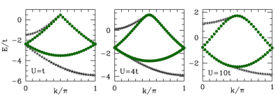
Figure 1: Location of the singularities of the spectral function in the thermodynamic limit for three values of $U$ in the plane ($k$,$E=-\omega$). The (green) circles correspond to the singularities of the $\mathcal{Z}_{k}(Q)$ (holon branch), while the black stars to the extrema of the excitation spectrum.

The full holon bandwidth is always $4t$ at all couplings, due to the particle-hole symmetry of the Hubbard model but the upper and lower branches of the holon band are not symmetrical at finite $U$. This observation is relevant for the correct interpretation of photoemission experiments, because an estimate of the effective hopping integral $t$ is usually performed by measuring the half bandwidth of the upper holon branch note3 leading to a sizable overestimate of $t$. In Fig. 2 we show the bandwidth $W_{h}$ of the upper holon branch (i.e. $\epsilon_{h}(\pi/2)-\epsilon_{h}(\pi)$) and the ratio between the spinon and the holon bandwidths $W_{s}/W_{h}$ as a function of the coupling $U/t$. Both quantities, which allow for a direct estimate of $t$ and $U/t$ from ARPES, show a remarkable (even non monotonic) dependence on the coupling constants.

Figure 2: Panel (a): holon bandwidth $W_{h}=\epsilon_{h}(\pi/2)-\epsilon_{h}(\pi)$ as a function of $U/t$. Panel (b): ratio between the spinon bandwidth $W_{s}=\epsilon_{s}(\pi)$ and $W_{h}$ as a function of $U/t$.

By comparing these results with the dispersion curves for SrCuO₂ reported in Ref. kim06 we can estimate the Hubbard effective coupling constants appropriate of this material: $t\sim 0.53$ eV and $U/t\sim 7$.

III The quasi-particle weight from Lanczos diagonalization

Unfortunately, the formal Bethe Ansatz solution does not lead to a practical way for the evaluation of the quasi-particle weight (5) at arbitrary couplings and therefore we resort to Lanczos diagonalizations in lattices up to $L=14$ sites. As previously noticed, we first have to devise a method to select the correct single spinon states at finite coupling $U/t$, for these states are not identified by a good quantum number at finite $U$. Our method is based on an adiabatic procedure starting from the strong coupling limit. We first perform a Lanczos diagonalization on the $(L-1)$-site Heisenberg model in the symmetry subspace of total momentum $Q$, leading to the numerical determination of $\phi_{H}$ and of the exact eigenstates of the one-hole Hubbard model for $U\to\infty$ via Eq. (3). In this limit, the single spinon states are indeed the lowest energy eigenstates at fixed spinon momentum $Q$ and can be easily obtained by Lanczos (or DMRG) technique, whilst at finite $U$ the relevant intermediate states are not necessarily in the low excitation energy portion of the Hubbard spectrum. Then we take advantage of the continuity of the one spinon states between the weak and strong coupling limit by adiabatically lowering the interaction strength $U$ and performing successive Lanczos diagonalizations for smaller and smaller couplings $U_{n}$. At the $n^{th}$ step we keep the exact eigenstate having the largest overlap with the eigenstate at the $(n-1)^{th}$ level. In this way we are able to identify the single spinon states down to small values of $U\sim t$, each state being uniquely identified by $Q$, i.e. by the momentum of the “parent” Heisenberg eigenstate.

A check on the validity of the single-spinon approximation comes from the completeness condition on the intermediate states:

$$n_{\downarrow}(k) = \langle\Psi_{0}|c_{k,\downarrow}^{\dagger}c_{k,\downarrow}|\Psi_{0}\rangle=\sum_{\{|\Psi_{1}\rangle\}}|\langle\Psi_{1}|c_{k,\downarrow}|\Psi_{0}\rangle|^{2}$$ (7)

$$\geq \sum_{Q}|\langle-k,Q|c_{k,\downarrow}|\Psi_{0}\rangle|^{2}$$

$$= \frac{1}{L-1}\sum_{Q}\mathcal{Z}_{k}(Q)$$

where $n_{\downarrow}(k)$ is the momentum distribution of the down spins at half filling and the equality holds if and only if the single spinon states included in the sum via the definition of the quasi-particle weight $\mathcal{Z}_{k}(Q)$ (5) exhaust the spectral weight at each $k$. The amount of violation of this sum rule quantifies the weight of all the neglected states in the Hilbert space due to the single-spinon approximation.

Figure 3: Momentum distribution $n_{\downarrow}(k)$ (black open circles) and $\frac{1}{L-1}\sum_{Q}\mathcal{Z}_{k}(Q)$ (red triangles) versus the hole momentum $k$ from Lanczos diagonalization, for $U=7t$ in a $L=14$ ring.

In Fig.3 we plot $n_{\downarrow}(k)$ and $\frac{1}{L-1}\sum_{Q}\mathcal{Z}_{k}(Q)$ restricted to the one spinon states: the violation of the completeness condition is smaller than $0.01$ at all $k$’s notek . Note how, even at fairly large values of $U/t$, the momentum distribution is considerably depressed for $k$ larger than the free electron Fermi momentum $k_{F}=\frac{\pi}{2}$, strongly reducing the spectral weight in the second half of the Brillouin zone. This feature is consistent with the photoemission experiments performed with high energy photons kim06 ; suga . Conversely, in the strong coupling limit $U\to\infty$, the momentum distribution becomes flat, $n_{\downarrow}(k)=1/2$, washing out this effect.

The dependence of the quasi-particle weight on the strength of the Coulomb repulsion has been investigated and is summarized in Fig.4 for strong and intermediate $U/t$ and for different lattice sizes.

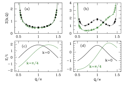
Figure 4: Panel (a): $\mathcal{Z}_{k}(Q)$ versus spinon momentum $Q$ for $U=100t$ and different lattice sizes ($\times$: L=6, $\blacktriangle$: L=8, $\blacksquare$: L=10, $\ast$: L=12, $\bullet$: L=14). Open (green) symbols for total momentum $k=\pi/4$ and full (black) symbols for $k=0$. Lines are polynomial fit to Lanczos data. Skewed boundary conditions are used in order to fix the same total momentum of the state $-k$ (relative to half filling) for all $L$’s. Panel (b): same as (a) for $U=7t$. Panel (c): binding energy at fixed $k$ referred to half filling versus spinon momentum $Q$ in the thermodynamic limit $E=E_{0}-E_{1}$ for $U=100t$. Panel (d): same as (c) for $U=7t$.

The quasi-particle weight has been evaluated by Lanczos diagonalization on lattices ranging from $L=6$ to $L=14$ sites. By using standard periodic boundary conditions, the total momentum of the state would be quantized in units of $2\pi/L$, making size scaling impractical. In order to avoid this problem we have adopted skewed boundary conditions: given an arbitrary hole momentum $k$ we choose the flux at the boundary in such a way to match $k$ with the quantization rule. Figure 4 reveals an astoundingly negligible size dependence and the expected vanishing of the quasi-particle spectral weight outside the spinon Fermi surface, with singularities at the Fermi momenta. While $\mathcal{Z}_{k}(Q)$ is almost independent on $k$ at large $U$, as expected SP_92 , it shows more structure for realistic values of $U/t$. The further peak (or shoulder) present for $k\leq\frac{\pi}{2}$ is indeed reminiscent of the free Fermi nature of the electrons at $U=0$. In the free particle limit, only one state provides a finite contribution to the spectral function: the holon sits at the bottom of the band ($k_{h}=\pi$) and the quasi-particle weight $\mathcal{Z}_{k}(Q)$ reduces to a delta function at $Q=\pi+k$. When such a form of $\mathcal{Z}_{k}(Q)$ is substituted in Eq. (4), the known free particle result is recovered. Remarkably, a remnant of the free particle peak in $\mathcal{Z}_{k}(Q)$ is still visible at $U=7t$, as shown in Fig. 4b.

IV Weak coupling limit

The Green’s function of one dimensional models has been thoroughly investigated by bosonization methods: while in the Luttinger liquid regime its asymptotic form is characterized by power law tails SC , precisely at half filling the Green’s function is known to display a more complex behavior due to the presence of a gap in the holon spectrum. At weak coupling, the holon dispersion near the bottom of the band shows a “relativistic ” structure:

$$\epsilon_{h}(k_{h})=\sqrt{v_{h}^{2}\delta k_{h}^{2}+m^{2}}$$ (8)

where $m$ is the charge gap and $\delta k_{h}=k_{h}\pm\pi$ is the holon momentum measured from the bottom of the band. Note that the holon spectrum (8) is shifted by $\mu=U/2$ with respect to our previous definition. In Fig. 5a we plot the exact Bethe Ansatz spectrum at $U=3t$ and the form (8) predicted by bosonization with suitably chosen parameters $m$,$v_{h}$.

In order to compare the results of our single spinon approximation with the bosonization form, it is convenient to introduce the single hole Green’s function in imaginary time:

$$G_{\downarrow}(k,\tau)=<\Psi_{0}|c^{\dagger}_{k,\downarrow}\,e^{-(H-\mu)\tau}\,c_{k,\downarrow}|\Psi_{0}>$$ (9)

According to bosonization ET , the Green’s function $G_{\downarrow}(k,\tau)$ of a hole of momentum close to $k_{F}=\pi/2$ acquires a factorized form in real space:

$$G^{R}_{\downarrow}(x,\tau) \equiv \int\frac{dk}{2\pi}G^{R}_{\downarrow}(k,\tau)e^{ikx}$$ (10)

$$= e^{i\frac{\pi}{2}x}\,G_{h}(x,\tau)\,G_{s}(x,\tau)$$

where the superscript $R$ identifies the contribution to the Green’s function due to right moving holes. Here, $G_{h}$ and $G_{s}$ just depend on holon and spinon degrees of freedom respectively. The spinon term is simply given by

$$G_{s}(x,\tau)=\frac{1}{\sqrt{v_{s}\tau+ix}}$$ (11)

while the holon contribution is predicted, by the form factor approach, to behave as

$$G_{h}(x,\tau)=\Gamma\,\sqrt{\frac{m}{v_{h}}}\,\int_{-\infty}^{\infty}\,d\theta\,e^{\left[\theta/2-m\tau\cosh\theta-im\frac{x}{v_{h}}\sinh\theta\right]}$$ (12)

with $\Gamma\sim 0.0585...$ ET . The question now arises whether our single spinon approximation is consistent with such a factorized form. By inserting a complete set of intermediate states into the definition (9) and adopting the single spinon approximation, the full Green’s function in imaginary time can be written as

$$G_{\downarrow}(k,\tau)=\frac{1}{L}\sum_{Q}{\mathcal{Z}_{k}(Q)}e^{-\left[\epsilon_{h}(k_{h})+\epsilon_{s}(Q)\right]\tau}$$ (13)

where the momentum conservation relation $k=k_{h}+Q$ is understood and the holon spectrum $\epsilon_{h}(k_{h})$ is now referred to the chemical potential $\mu$. Notice that, due to momentum conservation, the combined requirements of having $k\sim k_{F}=\frac{\pi}{2}$ and $k_{h}\sim-\pi$ (i.e. the hole sits near the bottom of the band) force $Q\sim\frac{3\pi}{2}$. By substituting the asymptotic forms (8) and $\epsilon_{s}\left(\frac{3\pi}{2}-q\right)=v_{s}q$ for $q\gtrsim 0$ we get:

$$G^{R}_{\downarrow}(x,\tau)=\,e^{i\frac{\pi}{2}x}\,\frac{m}{v_{h}}\,\int_{0}^{\pi}\frac{dq}{2\pi}e^{-\left[iqx+v_{s}q\tau\right]}\qquad$$ (14)

$$\qquad\times\,\int_{-\infty}^{\infty}\frac{d\theta}{2\pi}{\mathcal{Z}_{k}(Q)}\,\cosh\theta\,e^{\left[-im\frac{x}{v_{h}}\sinh\theta-m\tau\cosh\theta\right]}$$

where we set $\delta k_{h}\equiv-\frac{m}{v_{h}}\sinh\theta$. This form does indeed factorize in a holon and spinon part, as predicted by bosonization, provided the quasi-particle weight does:

$$\mathcal{Z}_{k}(Q)\sim Z_{h}(k_{h})\,Z_{s}(Q)$$ (15)

Notice that our approach, being based on a numerical evaluation of the quasi-particle weight, does not allow for an independent demonstration of such a factorized form. We just observe that the bosonization approach and the single-spinon approximation lead to the same result if we assume that Eq. (15) holds. Following Ref. essler we argue that the factorization of the quasi-particle weight at low energies (15) reflects the trivial structure of the holon-spinon scattering matrix in this limit.

As previously noticed, the spinon contribution to the quasi-particle weight gives rise to the square root divergence at the spinon Fermi surface, with leading behavior $Z_{s}\left(\frac{3\pi}{2}-q\right)\sim q^{-1/2}$ for $q\gtrsim 0$ which correctly reproduces Eq. (11) when the ultraviolet cut-off in Eq. (14) is disregarded. Matching Eqs. (12) and (14) then selects a unique form of the holon quasi-particle weight:

$$Z_{h}(k_{h})=\sqrt{2v_{h}}\,\frac{\sqrt{\epsilon_{h}(k_{h})-v_{h}\delta k_{h}}}{\epsilon_{h}(k_{h})}$$ (16)

with $\epsilon_{h}(k_{h})$ given by Eq. (8). The scale factor in Eq. (16) has been fixed by evaluating the Green’s function in the $\tau\to 0$ limit, where it coincides with the momentum distribution. In Fig. 5b we compare Eq. (16) with the numerical results for $Z_{h}(k_{h})$ obtained by Lanczos diagonalization at $U=3t$. No fitting parameters have been used: In order to obtain $Z_{h}(k_{h})$ we first evaluated $\mathcal{Z}_{k}(Q)$, as discussed in Section III, then we divided the result by $Z_{s}(Q)\sim q^{-1/2}$ evaluated at the spinon momentum $Q$ closest to the spinon Fermi point $Q_{F}=\frac{3\pi}{2}$. The two parameters $v_{h}$ and $m$ are independently obtained from the holon spectrum (also shown in Fig. 5a). As usual the Lanczos data display a very small size dependence and allow for a precise identification of the holon quasi-particle weight $Z_{h}(k_{h})$.

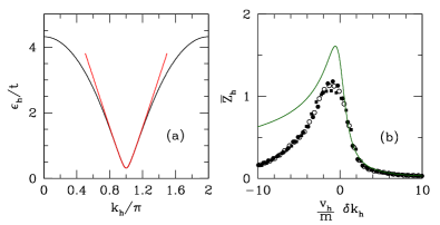
Figure 5: Panel (a): Holon spectrum $\epsilon_{h}(k_{h})$ of the Hubbard model at $U=3t$ from Bethe Ansatz (shifted by $\mu=U/2$) compared to the Lorentz form (8). The fitting parameters are $m=0.316t$ and $v_{h}=2.43t$. Panel (b): Dimensionless holon quasi-particle weight $\bar{Z}_{h}=\sqrt{\frac{m}{v_{h}}}Z_{h}$ in the single spinon approximation for $U=3t$ and lattice sizes $L=10$ (full squares), $L=12$ (empty circles), $L=14$ (full circles), compared to the bosonization result (16) (line).

The agreement between the two expressions is remarkable for $\delta k_{h}>0$ while some discrepancy is found for negative $\delta k_{h}$. Note however that the asymptotic form of the holon quasi-particle weight (16) holds only at low energies and weak coupling, while the comparison shown in Fig. 5 is performed for $U=3t$. The results at lower values of $U/t$ are plagued by severe finite size effects: in the $U\to 0$ limit, the holon mass $m$ vanishes exponentially and the dimensionless momentum scale $m/v_{h}$ vanishes as well. Therefore, at very weak coupling, the relevant holon momenta are constrained in an extremely small interval around $k_{h}=\pm\pi$, a range not easily accessible due to the momentum quantization rule in finite Hubbard rings.

V Results for ${\bf SrCuO_{2}}$

We are now ready to compare our results for the spectral function of the 1D Hubbard model with precise photoemission data recently obtained for ${\rm SrCuO_{2}}$ kim06 . A preliminary study, based on the strong coupling limit of the Hubbard model, pointed out some discrepancies, related to the peak heights and widths kim06 .

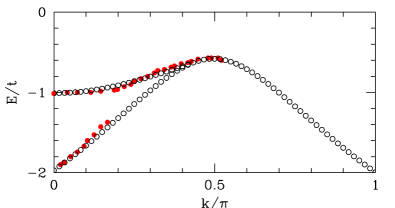
Figure 6: Locus of singularities of the spectral function for the Hubbard model at $U=3.7$ eV and $t=0.53$ eV (open circles) compared to the experimental results by Kim et al. kim06 (full circles) for $k_{\perp}=0.1$.

Fig. 6 shows the singularity loci of the 1D Hubbard model with the parameters $t=0.53$ eV and $U=3.7$ eV, together with the ARPES results from Kim et al. kim06 . The nice agreement suggests that this material indeed represents a good experimental realization of the simple one dimensional Hubbard model. The effects due to inter-chain coupling, phonons, finite temperature and other perturbations appears rather small and mostly limited to the spinon branch. We remark that the same material has been already theoretically investigated on the basis of the Hubbard and t-J model by several groups kim06 ; popovich ; koitzsch leading to different sets of parameters both for the hopping integral $0.3{\rm eV}\lesssim t\lesssim 0.7{\rm eV}$ and for the Coulomb repulsion $2{\rm eV}\lesssim U\lesssim 6.5{\rm eV}$. Our analysis shows that both spin and charge fluctuations play a key role in determining the line shape of the spectral function of the Hubbard model, even at moderately high values of the coupling $U/t$.

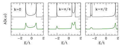
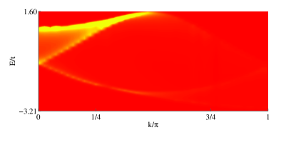
Figure 7: Upper panels: $A(k,\omega)$ calculated via Eq. (4) for three representative values of the momentum $k$ and $U=7t$. The binding energy is $E=-\omega$. The lower curves are the convolution of the spectral function with a Gaussian with FWHM equal to $0.12t$ corresponding to an experimental resolution of $60$ meV kim06 . Lower panel: density plot of the spectral function on the $(k,E)$ plane with the experimental broadening.

In Fig.7 the spectral function has been plotted versus the binding energy $E=-\omega$ for three representative values of the total hole momentum $k$. The experimental line broadening reported in Ref.kim06 has been also included in the Hubbard model results, leading to a merging of close peaks. The density plot clearly reproduces the overall shape defined by the singularities of the spectral function shown in Fig.6. As expected, most of the spectral weight is indeed concentrated in the first half of the Brillouin zone between the holon and the spinon band. Although the relative intensity of the ARPES signal at the two singularities depends on the details of the band structure, the power-law nature of the divergences implies that the intrinsic width of each peak is always comparable with the separation between the holon and the spinon branch $\Delta\omega\sim\epsilon_{h}(k+\frac{\pi}{2})-[\epsilon_{h}(\pi)+\epsilon_{s}(\pi+k)]$. The average intensity can be estimated on the basis of the sum rule (7) and scales as $(\Delta\omega)^{-1/2}$, getting smaller when the two branches separate, as shown both in experiments kim06 and in numerical calculations Matsueda .

VI Conclusions

The single spinon approximation, combined to Bethe Ansatz results and Lanczos diagonalizations allows to obtain very accurate results for the dynamic properties of a single hole in the one dimensional Hubbard model. The Lehmann representation of the spectral function (2) shows that two separate ingredients combine to define the overall shape of $A(k,\omega)$: the excitation spectrum and the quasi-particle weight. The idea at the basis of our method is to limit the size effects that plague numerical results by dealing with these two quantities separately: in the 1D Hubbard model the excitation spectrum is given exactly by the Bethe Ansatz equations in the thermodynamic limit LW , while the quasi-particle weight is obtained, in the single spinon approximation, by Lanczos diagonalization. Size effects are shown to be negligible and the accuracy of the approximation can be checked a posteriori by a frequency sum rule (7). Our expression for the spectral function of the 1D Hubbard model (4) is consistent with the structure predicted by bosonization ET at weak coupling, provided the quasi-particle weight ${\mathcal{Z}}_{k}(Q)$ factorizes as shown in Eq. (15). A numerical test carried out at $U=3t$ does not show a convincing quantitative agreement with the result obtained by the form factor approach ET , possibly due to the difficulty to achieve the $U\to 0$ limit.

The extension to finite doping is straightforward but in principle this approach can be also generalized to other fermionic lattice models, in one or more dimensions, provided the relevant states entering the quasi-particle weight in the strong coupling limit can be easily classified. This would be the case of the extended Hubbard model (i.e. a Hubbard model with nearest neighbor Coulomb repulsion) or in the presence of lattice dimerization. Clearly, for non integrable models, no analytical information on the excitation spectrum is available and a size scaling on the energy spectrum is also required. A study of such generalizations may be useful to understand the role of some perturbation on the spectral function of correlated electron models.

The specific example of SrCUO₂ shows that our method allows for a direct comparison between theory and ARPES experiments and for an accurate determination of the Hubbard parameters which best describe the hole dynamics in the material. The spectral function derived here provides a natural explanation of the observed reduction of the spectral weight in a half of the Brillouin zone and of the broad line-shape detected in experiments. Future applications of this method to the case of cold atoms in optical traps may help in pointing out the peculiar features of one dimensional physics in other experimental realizations of correlated one dimensional Fermi gases.

We thank C. Kim and F.H.L Essler for stimulating correspondence.

References

- (1) See for instance J. Solyom, Adv. Phys. 28, 201 (1979).
- (2) C.Kim, A.Y.Matsuura, Z.-X.Shen, N.Motoyama, H.Eisaki, S.Uchida, T.Tohyama and S. Maekawa, Phys. Rev. Lett. 77, 4054 (1996).
- (3) B.J.Kim, H.Koh, E.Rotenberg, S.-J.Oh, H.Eisaki, N.Motoyama, S.Uchida, T. Tohyama, S. Maekawa, Z.-X.Shen and C.Kim, Nature Physics, 2, 397 (2006).
- (4) T.E.Kidd, T.Valla, P.D.Johnson, K.W.Kim, G.D.Gu and C.C.Homes, Phys. Rev. B77, 054503 (2008).
- (5) M.Hoinkis, M.Sing, S.Glawion, L.Pisani, R.Valenti, S. van Smaalen, M.Klemm, S.Horn and R.Claessen, Phys. Rev. B75, 245124 (2007).
- (6) S.Suga, A.Shigemoto, A.Sekiyama, S.Imada, A.Yamasaki, A.Irizawa and S.Kasai, Phys. Rev. B70, 155106 (2004).
- (7) H.Matsueda, N.Bulut, T.Tohyama and S. Maekawa, Phys. Rev. B72, 075136 (2005).
- (8) S.Sorella and A.Parola, J. Phys.:Cond. Matt. 4,3589 (1992).
- (9) F.H.L.Essler and A.M.Tsvelik, Phys. Rev. B65, 115117 (2002).
- (10) The limitation to intermediate and strong coupling is a technical one: at weak coupling size effects become more relevant and the adiabatic procedure employed in this work might fail.
- (11) E.H.Lieb and F.Y.Wu, Phys. Rev. Lett. 20, 1445 (1968).
- (12) F.Woynarovich, J. Phys. C: Solid State Phys, 15, 85, (1982).
- (13) F.Woynarovich, J. Phys. C: Solid State Phys, 16, 5293 (1983).
- (14) F.H.L.Essler, H.Frahm, F.Göhmann, A.Klümper and V.E.Korepin, The One-Dimensional Hubbard Model, Cambridge University Press, (2005).
- (15) F.D.M. Haldane Phys. Rev. Lett. 60, 635 (1988).
- (16) F.D.M.Haldane and M.R.Zirnbauer, Phys. Rev. Lett. 71, 4055 (1993).
- (17) In one dimension and exactly at all spin configurations are degenerate: however in the limit the spin degeneracy is lifted and the ground state of the Heisenberg model is singled out.
- (18) M.Ogata and H.Shiba, Phys. Rev. B41, 2326 (1990).
- (19) With the notation adopted in this work, at , for .
- (20) Our definition of the spinon momentum , which for must reduce to the total momentum of the Heisenberg wave function in Eq. (3), differs from the one usually adopted in Bethe Ansatz studies () woy : .
- (21) S.Sorella and A.Parola, Phys. Rev. Lett. 76, 4604 (1996); Phys. Rev. B57, 6444 (1998).
- (22) At the special values of defined by the coincidence of the two singularities the critical exponent changes from to .
- (23) In experiments the lower branch is not detected because it usually overlaps with other valence bands of the compound.
- (24) The accuracy of the single spinon approximation is similar also at weaker coupling: for the completeness condition (7) is violated at most by at all ’s.
- (25) Z.V.Popović, V.A.Ivanov, M.J.Kostantinović, A.Cantarero, J.Martínez-Pastor, D.Olguín, M.I.Alonso, M.Garriga, O.P.Khuong, A.Vietkin and V.V.Moshchalkov, Phys. Rev. B63, 165105 (2001).
- (26) A.Koitzsch, S.V. Borisenko, J.Geck, V.B.Zabolotnyy, M.Knupfer, J.Fink, P.Ribeiro, B.Büchner and R.Follath, Phys. Rev. B73, 201101(R) (2006).