PostScript file created: ;  time 1053 minutes

STATISTICAL DISTRIBUTIONS OF EARTHQUAKE NUMBERS:

CONSEQUENCE OF BRANCHING PROCESS

Yan Y. Kagan,

Department of Earth and Space Sciences, University of California,

Los Angeles, California 90095-1567, USA;

Emails: ykagan@ucla.edu, kagan@moho.ess.ucla.edu

Abstract.

We discuss various statistical distributions of earthquake numbers. Previously we derived several discrete distributions to describe earthquake numbers for the branching model of earthquake occurrence: these distributions are the Poisson, geometric, logarithmic, and the negative binomial (NBD). The theoretical model is the ‘birth and immigration’ population process. The first three distributions above can be considered special cases of the NBD. In particular, a point branching process along the magnitude (or log seismic moment) axis with independent events (immigrants) explains the magnitude/moment-frequency relation and the NBD of earthquake counts in large time/space windows, as well as the dependence of the NBD parameters on the magnitude threshold (magnitude of an earthquake catalog completeness). We discuss applying these distributions, especially the NBD, to approximate event numbers in earthquake catalogs. There are many different representations of the NBD. Most can be traced either to the Pascal distribution or to the mixture of the Poisson distribution with the gamma law. We discuss advantages and drawbacks of both representations for statistical analysis of earthquake catalogs. We also consider applying the NBD to earthquake forecasts and describe the limits of the application for the given equations. In contrast to the one-parameter Poisson distribution so widely used to describe earthquake occurrence, the NBD has two parameters. The second parameter can be used to characterize clustering or over-dispersion of a process. We determine the parameter values and their uncertainties for several local and global catalogs, and their subdivisions in various time intervals, magnitude thresholds, spatial windows, and tectonic categories. The theoretical model of how the clustering parameter depends on the corner (maximum) magnitude can be used to predict future earthquake number distribution in regions where very large earthquakes have not yet occurred.

Short running title: Distributions of earthquake numbers

Key words:

Probability distributions $<$GEOPHYSICAL METHODS, Statistical seismology $<$SEISMOLOGY, Theoretical seismology $<$SEISMOLOGY, North America $<$GEOGRAPHIC LOCATION, Probabilistic forecasting $<$GEOPHYSICAL METHODS, Earthquake interaction, forecasting, and prediction $<$SEISMOLOGY

1 Introduction

Earthquake forecasts are important in estimating hazard and risk and in making informed decisions to manage emergency response. How can we establish standards for reporting and testing earthquake forecasts? One significant effort began in California, where the Regional Earthquake Likelihood Models (RELM) project published a dozen models for earthquake rate density and a likelihood based method for prospective testing (Field, 2007; Schorlemmer and Gerstenberger, 2007; Schorlemmer et al., 2007; Schorlemmer et al., 2009). The Collaboratory for Study of Earthquake Predictability (CSEP) is currently extending the tests to several natural laboratories around the globe.

One standard test is to compare the number of predicted earthquakes with the actual number of events during the test period. To do so we need to know the statistical distribution of earthquake numbers.

The standard assumption long used in earthquake hazard analysis (Cornell, 1968) is that earthquake occurrence is reasonably well described by the Poisson distribution. However, it has also been known for a long time that earthquakes are clustered in time and space: their distribution is over-dispersed compared to the Poisson law. One conventional way to treat this problem is to decluster an earthquake catalog (Schorlemmer et al., 2007). But there are several declustering procedures, mostly based on ad-hoc rules. Hence declustered catalogs are not unique and usually not fully reproducible. Therefore, it is important to derive and investigate earthquake number distribution in real earthquake catalogs.

Kagan (1996), Jackson and Kagan (1999), and Kagan and Jackson (2000) have all used the negative binomial distribution (NBD) to approximate earthquake numbers in catalogs. The NBD has a higher variance than the Poisson law and can be shown (Kagan, 1973a,b) to result from the branching nature of earthquake occurrence.

In principle, several other over-dispersed discrete distributions, such as generalized Poisson distributions (Consul, 1989) or generalized negative-binomial distributions (Tripathi, 2006; Hilbe, 2007) can be used to approximate earthquake numbers. However, the NBD has the advantage of relative simplicity and is supported by theoretical arguments (Kagan, 1973a,b). As we discuss below, in addition to negative-binomial and Poisson distributions, several other statistical discrete distributions can describe earthquake numbers. A general discussion of such distributions can be found in Johnson et al. (2005) and Kotz et al. (2006).

Over the years many papers have analyzed various aspects of earthquake numbers distributions; for example, see Vere-Jones (1970), Shlien and Toksöz (1970), Dionysiou and Papadopoulos (1992). These publications investigated the distributions empirically by counting earthquake numbers in catalogs and trying to approximate them by various statistical laws. Here we explain these distributions as a consequence of the stochastic branching model.

Therefore, in addition to the NBD and the Poisson distributions, in this study we will investigate the geometric and logarithmic distributions in several earthquake catalogs and show their applicability in certain conditions. After presenting the theoretical derivation of these distributions, we explore the statistical parameter estimation for these laws. Then we apply these methods to several earthquake catalogs. Two global (CMT and PDE) and one local Californian catalog are studied and the results are displayed in tables and diagrams. These results can be used in earthquake forecast testing (Schorlemmer et al., 2007; Schorlemmer et al., 2009; Kagan et al., 2009).

2 Theoretical considerations

2.1 Generating function for the NBD

Several stochastic models of earthquake occurrence were proposed and almost all were based on the theory of branching processes (Kagan, 2006). Branching is expected to model the well-known property of primary and secondary clustering for aftershock sequences: a strong aftershock (or foreshock) tends to have its own sequence of dependent events. These multidimensional models are

$\bullet$ (a) The supercritical point process branching along the magnitude axis, introduced by Kagan (1973a,b) and shown in Fig. 1a. Earthquake occurrence constitutes a down-going cascade in this model.

$\bullet$ (b) Critical (or rather slightly subcritical) point process branching along the time axis (Hawkes 1971; Kagan and Knopoff, 1987; Ogata, 1988) – often called the Hawkes self-exciting process or the ETAS model (see Fig. 1b). Hawkes and Tukey debate (see discussion section in Kagan, 1973b) the difference between branching in earthquake size and that in time. Bremaud and Massoulie (2001) recently proposed a variant of Hawkes’ process with no independent events (immigrants). However, in earthquake catalogs limited in time-span, we need to introduce independent events. Otherwise, models would be highly non-unique.

Both models shown in Fig. 1 use the Poisson cluster process to approximate earthquake occurrence. Earthquake clusters are assumed to follow the Poisson occurrence. Earthquakes within a cluster are modeled by a multidimensional branching process, which reproduces a temporal-spatial pattern of dependent events (mostly aftershocks) around the initial one in a sequence (Kagan, 1973a,b; Kagan and Knopoff, 1987; Ogata, 1988, 1998).

In one form or another, these models employ the classical statistical properties of earthquake occurrence: the Gutenberg-Richter (G-R) relation and Omori’s law. Model (a) reproduces the G-R relation as the result of a supercritical branching along the magnitude axis, while the temporal distribution (the Omori-type law) must be imposed. In model (b) both the temporal and magnitude distributions are imposed.

The simplest way to describe discrete distributions is by using the probability generating function (Bartlett, 1978; Evans et al., 2000). Given the generating function $\phi\,(z)$, the probability function $f\,(k)$ can be obtained as

$$f\,(k)\ =\ {1\over{k!}}\left[{{d^{k}\phi\,(z)}\over{dz^{k}}}\right]_{z=0}\,.$$ (1)

Following the graph of inter-earthquake connections as shown in Fig. 1a, we investigate the earthquake numbers distributions for space-time intervals larger that the average dimensions of earthquake clusters. Thus, we neglect space-time differences between cluster members. We assume that the independent (mainshocks) and dependent (foreshocks-aftershocks) events are occurring along the $\Xi\,=\,\log M$ axis ($M$ is the scalar seismic moment) with a constant rates

$$\nu\,(d\,\Xi)\ = \ \nu\,\cdot\,d\,\Xi\ =\ {\rm const}\,\cdot\,d\,\Xi\,,$$

$$\beta\,(d\,\Xi)\ = \ \beta\,\cdot\,d\,\Xi\ =\ {\rm const}\,\cdot\,d\,\Xi\,,$$ (2)

$${\rm for}\ \Xi\,<\,\Xi_{\rm m}\,,$$

where $\Xi_{\rm m}$ is the logarithm of the maximum seismic moment, $M_{m}$; $\nu$ and $\beta$ are rates of independent and dependent events, respectively.

Events occurrence can be modeled as an ‘immigration and birth’ process, where independent, spontaneous earthquakes (mainshocks) are treated as ‘immigrants’. Any immigrant may spawn offspring, who may spawn their own offspring, etc., with the whole family making up a cluster. Seismologists generally call the largest family member the ‘mainshock’, and the preceding smaller events the ‘foreshocks’, and subsequent members the ‘aftershocks’. In this case the conditional generating function for the number of events with $\Xi\geq\Xi_{c}$ in a cluster, including the mainshock, is (Bartlett, 1978, Eq. 3.4(7), p. 76)

$$\phi\,(z\,|\,\Xi_{c})\ =\ {{z\,(M_{c}/M)^{\beta}}\over{1\,-\,z\,[\,1\,-\,(M_{c}/M)^{\beta}\,]}}\,,$$ (3)

where $\beta$ is the index of the seismic moment distribution, $\beta={2\over 3}b$;  $b$ is the parameter of the G-R law (Kagan and Jackson, 2000; Bird and Kagan, 2004), and $M_{c}$ is the moment detection threshold of a seismographic network ($M\geq M_{c}$). In this formula we modify Bartlett’s equation for the ‘birth and immigration’ (but no ‘deaths’) population process.

In future calculations here we take

$$\beta\ =\ 0.62\,:$$ (4)

the value suggested by results in the Bird and Kagan (2004) and Kagan et al. (2009).

Equation (3) characterizes the geometric distribution, with the probability function

$$f\,(k)\ =\ (1-p)^{k-1}p\quad{\rm for}\quad k=1,2,3,\dots\,$$ (5)

A more common form of the geometric distribution (Evans et al., 2000) is

$$f\,(k)\ =\ (1-p)^{k}p\quad{\rm for}\quad k=0,1,2,\dots\,$$ (6)

It would be appropriate for the number of dependent shocks in a cluster. Its conditional generating function is

$$\phi\,(z\,|\,\Xi_{c})\ =\ {{(M_{c}/M)^{\beta}}\over{1\,-\,z\,[\,1\,-\,(M_{c}/M)^{\beta}\,]}}\,.$$ (7)

The geometric distribution is a discrete analog of the exponential distribution for continuous variables. For a small $p$-value

$$f\,(k)\ \approx\ p\,\exp-k\,p\,.$$ (8)

For the distribution of the total number of events in an earthquake catalog we obtain (Bartlett, 1978, Ch. 3.41, p. 83)

$$\phi\,(z)\ = \ \exp\int_{\Xi_{c}}^{\Xi_{m}}[\,\phi\,(z\,|\,\Xi)\,-\,1\,]\,\nu\,d\,\Xi$$ (9)

$$= \ \exp\left\{\left[{{\log\left(1\,-\,z\,[\,1\,-\,(M_{c}/M_{m})^{\beta}\,]\right)}\over-{\beta\,(\,\Xi_{m}-\Xi_{c}\,)}}\,-1\,\right]\,\nu\,(\,\Xi_{m}-\Xi_{c}\,)\right\}$$

$$= \ \left[{{(M_{c}/M_{m})^{\beta}}\over{1\,-\,z\,[\,1\,-\,(M_{c}/M_{m})^{\beta}\,]}}\right]^{\nu/\beta}\,.$$

The above generating function is for the NBD.

In this derivation we assume that the ‘immigration and birth’ process starts at the maximum moment: we assume the moment distribution to be a truncated Pareto distribution with a ‘hard’ limit on the maximum moment (Kagan and Jackson, 2000; Zaliapin at al., 2005; Kagan, 2006). However, a more appropriate seismic moment distribution (a tapered Pareto distribution) uses a ‘soft’ limit or a corner moment (ibid., Bird and Kagan, 2004). To consider this, Kagan and Jackson (2000, Eq. 29) propose some modification of the NBD formulas.

The last line in (9) means that the distribution of events (counting mainshocks as well) in earthquake clusters would be logarithmic (or logarithmic series) with the probability function

$$f\,(k)\ =\ {{\left[1\,-\,(M_{c}/M_{m})^{\beta}\right]^{k}}\over{k\,\log(M_{c}/M_{m})^{\beta}}}\ =\ {{\left[1\,-\,(M_{c}/M_{m})^{\beta}\right]^{k}}\over{k\,\beta\,(\Xi_{m}-\Xi_{c})}}\quad{\rm for}\quad k=1,2,3,\dots\,.$$ (10)

The standard form of the logarithmic distribution (Evans et al., 2000) is

$$f\,(k)\ =\ {{-1}\over{\log(1-p)}}\cdot{{p^{k}}\over k}\quad{\rm for}\quad k=1,2,3,\dots\,.$$ (11)

For a small moment threshold, the logarithmic distribution can be approximated by a tapered Pareto distribution (Zaliapin et al., 2005)

$$f\,(k)\ \approx\ \left\{\,k\log\left[\,(M_{m}/M_{c})^{\beta}\,\right]\exp\left[\,k\,(M_{c}/M_{m})^{\beta}\,\right]\right\}^{-1}\quad{\rm for}\quad k=1,2,3,\dots\,,$$ (12)

i.e., the clusters with small and intermediate mainshocks follow the Pareto style heavy-tail distribution. The exponential tail should be observed only for clusters with large mainshocks having a magnitude close to maximum.

The average size for a group of dependent events is

$$S\,(k)\ =\ {{\left[\,(M_{m}/M_{c})^{\beta}-1\right]}\over{\beta\,(\Xi_{m}-\Xi_{c})}}\,.$$ (13)

It is clear from Eqs. 10 and 13 that the number of dependent events decreases as $M_{c}\to M_{m}$: the largest earthquakes are distributed according to the Poisson law.

The Poisson distribution has the probability function of observing $k$ events as

$$f\,(k)\ =\ {{\lambda^{k}\exp(-\lambda)}\over{k!}}\,.$$ (14)

For this distribution its mean and variance are equal to its rate $\lambda$.

What are the distributions of earthquake numbers for the branching-in-time model (see Fig. 1b)? Can we calculate these distributions similarly to model (a)? Indeed, when the first event in a sequence of earthquakes is the largest one, as is often the case, there is little ambiguity in calling it a mainshock, and the other dependent events may be called aftershocks, though some of them are actually aftershocks of aftershocks. In such a case there is little difference between (a) and (b) models. If, however, the first event in a sequence is smaller than the subsequent events, it is typically called a foreshock. Retrospectively, it is relatively easy to subdivide an earthquake catalogue into fore-, main-, and aftershocks. However, in real-time forecasting it is uncertain whether the most recent event registered by a seismographic network is a foreshock or a mainshock. Although the subsequent triggered events are likely to be smaller and would thus be called aftershocks, there is a significant chance that some succeeding earthquakes may be bigger than the predecessors that triggered them (Kagan, 1991).

The difficulty in model (b) is that some connections between events are not observable. Suppose that there is a potential foreshock-mainshock pair: a larger earthquake is preceded by a smaller one. However, the first event is below the magnitude threshold and the larger earthquake is above the threshold. Then this second event would be treated as independent (immigrant); that is, our calculations would miss this connection (Kagan, 1991; Sornette and Werner, 2005; Kagan, 2006). It is possible that the number of such missed connections is small, and the distributions are similar to those derived above. Nevertheless, such distribution estimates for this model would be approximate. For the branching-in-magnitude model (Fig. 1a), the derived expressions are exact.

The equations obtained in this subsection are based on the theory of population processes. In simple models of such processes (Bartlett, 1978), we assume that individuals start to reproduce immediately after their birth. This is not the case for an earthquake occurrence: after a large event, the aftershocks even large ones cannot be observed for a period of time (Kagan, 2004). Moreover, earthquakes are not instantaneous, point events; and their rupture takes time. Hence, the derived formulas would over-estimate the number of dependent events. However, as we will see below, during analysis of the earthquake catalogs the theoretical models provide some valuable insight into the quantitative behavior of earthquake occurrence.

2.2 NBD distribution expressions

There are many different (often confusing) representations of the NBD (see several examples in Anscombe, 1950; Shenton and Myers, 1963). The most frequently used (we call it standard) form of the probability density function for the NBD generalizes the Pascal distribution (Feller, 1968, Eq. VI.8.1; Hilbe, 2007, Eq. 5.19):

$$f\,(k)\ = \ {{\tau\,(\tau+1)\dots(\tau+k-2)\,(\tau+k-1)}\over{k!}}\,\times\,\theta^{\tau}(1-\theta)^{k}\ =\ {\tau+k-1\choose\tau-1}\,\times\,\theta^{\tau}(1-\theta)^{k}\$$

$$= \ {\tau+k-1\choose k}\,\times\,\theta^{\tau}(1-\theta)^{k}\ \ =\ \ {{\Gamma(\tau+k)}\over{\Gamma(\tau)\,k!}}\,\times\,\theta^{\tau}(1-\theta)^{k}\,,$$ (15)

where $k=0,1,2,\dots$, $\Gamma$ is the gamma function, $0\leq\theta\leq 1$, and $\tau>0$. If the parameter $\tau$ is integer, then this formula (Pascal distribution) is the probability distribution of a certain number of failures and successes in a series of independent and identically distributed Bernoulli trials. For $k+\tau$ Bernoulli trials with success probability $\theta$, the negative binomial gives the probability for $k$ failures and $\tau$ successes, with success on the last trial. If $\tau=1$, this equation corresponds to (5): the geometric distribution. Therefore, the latter distribution can be considered a special case of the NBD.

The average of $k$ for the NBD is

$$E(k)\ =\ m_{1}\ =\ \tau\,{{1-\theta}\over\theta},$$ (16)

and its variance

$$D(k)\ =\ m_{2}\ =\ \tau\,{{1-\theta}\over\theta^{2}}.$$ (17)

The negative binomial distribution generally has a larger standard deviation than the Poisson law. Thus, it is often called an ‘over-dispersed Poisson distribution’ (Hilbe, 2007). For $\theta\to 1$ and $\tau(1-\theta)\to\lambda$ expression (15) tends to (14) (Feller, 1968, p. 281); the negative binomial distribution becomes the Poisson distribution; the latter distribution is a special case of the former.

Anraku and Yanagimoto (1990, Eq. 1.1) and Hilbe (2007, Eqs. 5.9 or 5.29) propose the following distribution density form, which they obtain as a mixture of the Poisson distributions with the gamma distributed rate parameter $\lambda$ (see, for example, Hilbe, 2007, Eqs. 5.1–5.9 or 7.21–7.33)

$$f\,(k)\ =\ {{\Gamma(1/\alpha+k)}\over{\Gamma(1/\alpha)\,k!}}\cdot{{\lambda^{k}}\over{(\lambda+1/\alpha)^{k}\,(1+\alpha\lambda)^{1/\alpha}}}\ =\ {{\lambda^{k}}\over{k!}}\cdot{{\Gamma(1/\alpha+k)}\over{\Gamma(1/\alpha)\,(\lambda+1/\alpha)^{k}}}\cdot{{1}\over{(1+\alpha\lambda)^{1/\alpha}}}\,,$$ (18)

which converges to the geometric distribution if $\,\alpha=1\,$, but to the Poisson distribution (14) when $\,\alpha\to 0\,$,

$$f\,(k)\ =\ {{\lambda^{k}}\over{k!}}\cdot 1\cdot{{1}\over{\exp(\lambda)}}\,.$$ (19)

Comparison with (15) shows that $\,\alpha=1/\tau\,$ and $\,\lambda=\tau\,(1-\theta)/\theta\,$. Distribution (18) is called an alternative form of the NBD in Wikipedia and we accept this term for our purposes.

In addition to the above representations of the NBD, we use Evans’ (1953) expressions. Evans provides the parameter uncertainty equations for the estimates by the moment method. The formula for the probability density is

$$f\,(k)\ =\ {{\Gamma(\lambda/a+k)}\over{\Gamma(\lambda/a)\,k!}}\times{{[a/(1+a)]^{k}}\over{(1+a)^{\lambda/a}}}\,,$$ (20)

If we make $a=\alpha\,\lambda$, this equation converts to (18).

The probability generating function (Bartlett, 1978) for the NBD standard form is

$$\phi\,(z)\ =\ \left[{\theta\over{1-z(1-\theta)}}\right]^{\tau}\,,$$ (21)

For the alternative form (18) of the NBD the generating function is

$$\phi\,(z)\ =\ {1\over{[1+\alpha\lambda-z\alpha\lambda]^{1/\alpha}}}\,,$$ (22)

Comparing (21) with (9), it is clear that if the moment threshold is close to $M_{m}$, the NBD approaches the Poisson distribution for earthquake counts. This is confirmed by extensive seismological practice (see also Figs. 13 and 14 below).

After comparing (21) with (9), we propose the following relations between the parameters

$$\theta\ =\ \left({M_{c}\over M_{m}}\right)^{\beta}\,,$$ (23)

and

$$\tau\ =\ \nu/\beta\,.$$ (24)

However, as mentioned at the end of Subsection 2.1, such relations are valid only when larger shocks start producing dependent events immediately after their rupture. In earthquake catalogs there is a significant delay of aftershock generation (Kagan, 2004). Thus, these expressions are over-estimated. Moreover, in all available earthquake catalogs there are very few or no mainshocks with a size approaching the maximum magnitude. Therefore, we would not expect the observational $\theta$-estimates to be close to that of (23). However, as we will see the dependence of $\theta$ on the magnitude threshold, the maximum magnitude, and $\beta$ is visible in earthquake records.

2.3 Statistical parameter estimation

For the Poisson distribution (14) the estimate of its parameter is the average earthquake rate per time interval ${\Delta T}$

$$\hat{\lambda}\ =\ {{n\,{\Delta T}}\over T}\,,$$ (25)

where $T$ is the time-span and $n$ is total number of events in a catalog. The estimate of $p$ for the geometric distribution’s (5) is

$$\hat{p}\ =\ {1\over{1+m_{1}}}\,,$$ (26)

where $\,m_{1}=\hat{\lambda}\,$ is the average (the first moment).

For the logarithmic distribution (11) there is no simple expression to evaluate its parameter $p$. Patil (1962, Table 1) and Patil and Wani (1965, Table 2) propose tables for calculating the maximum likelihood estimate (MLE) of the parameter after determining the average number of events.

For the standard form (15) of the NBD, we use (16) and (17) to obtain the estimates of the NBD parameters by the moment method

$$\hat{\theta}\ =\ {{m_{1}}\over{m_{2}}}\,,$$ (27)

and

$$\hat{\tau}\ =\ {{m_{1}^{2}}\over{m_{2}-m_{1}}}\,,$$ (28)

where $m_{1}$ and $m_{2}$ are the average and variance of the empirical number distribution. Below we sometimes would use the term moment estimate for the estimate by the moment method. For the Poisson process, $m_{2}=m_{1}$. Hence the estimate (28) would be unstable if the NBD process approaches the Poisson one, and the estimate uncertainty would be high.

For the alternative form of the NBD (18), we obtain the following moment estimates

$$\hat{\lambda}\ =\ m_{1}\,,$$ (29)

and

$$\hat{\alpha}\ =\ {{m_{2}-m_{1}}\over m_{1}^{2}}\,.$$ (30)

Evans’ (1953) parameter $a$ is estimated similarly to (30)

$$\hat{a}\ =\ {{m_{2}-m_{1}}\over m_{1}}\ =\ {m_{2}\over m_{1}}-1\,.$$ (31)

Evans (1953, p. 203, see ‘Estimation by Method 1’) derives approximate estimates of the parameters’ uncertainties

$$\sigma_{\lambda}\ =\ \sqrt{\lambda(a+1)/N}\,.$$ (32)

and

$$\sigma_{a}\ \approx\ \sqrt{2(a+1)/N+a(a+1)(3a+2)/(\lambda N)}\,.$$ (33)

as well as the covariance between these two estimates

$${\rm Cov}(\hat{\lambda},\,\hat{a})\ \approx\ a(a+1)/N\,.$$ (34)

In these equations $N$ is the number of time intervals with earthquake counts.

The maximum likelihood estimate (MLE) of any parameters for the discussed distributions can be obtained by maximizing the log-likelihood function

$${\ell}\ =\ \log\,\prod_{j=0}^{\infty}\,[\,f\,(k_{j})\,]^{P(k_{j})\,}\ =\ \sum_{j=0}^{\infty}\,P(k_{j})\,\log\,f\,(k_{j})\,,$$ (35)

where $P(k_{j})$ is the observational frequency of earthquake numbers in interval $j$. Function $f(k)$ is defined by the expression (14), (15), (18), or (20) for the Poisson, the standard NBD, the alternative NBD, and Evans’ formula, respectively. To evaluate parameter uncertainties we need to obtain the Hessian matrix (the second partial derivatives of the likelihood function) of the parameter estimates (Wilks, 1962; Hilbe, 2007).

3 Earthquake catalogs

We studied earthquake distributions and clustering for the global CMT catalog of moment tensor inversions compiled by the CMT group (Ekström et al., 2005). The present catalog contains more than 28,000 earthquake entries for the period 1977/1/1 to 2007/12/31. Earthquake size is characterized by a scalar seismic moment $M$. The moment magnitude can be calculated from the seismic moment (measured in Nm) value as

$$m_{W}\ =\ (2/3)\cdot\log_{10}M-6\,.$$ (36)

The magnitude threshold for the catalog is $m5.8$ (Kagan, 2003).

The PDE worldwide catalog is published by the USGS (U.S. Geological Survey, 2008); in its final form, the catalog available at the time this article was written ended on January 1, 2008. The catalog measures earthquake size, using several magnitude scales, and provides the body-wave ($m_{b}$) and surface-wave ($M_{S}$) magnitudes for most moderate and large events since 1965 and 1968, respectively. The moment magnitude ($m_{W}$) estimate has been added recently.

Determining one measure of earthquake size for the PDE catalog entails a certain difficulty. For example, Kagan (1991) calculates a weighted average of several magnitudes to use in the likelihood search. Kagan (2003) also analyzes systematic and random errors for various magnitudes in the PDE catalog. At various times different magnitudes have been listed in the PDE catalog, and establishing their relationships is challenging. Therefore, we chose a palliative solution: for each earthquake we use the maximum magnitude among those magnitudes shown. This solution is easier to carry out and the results are easily reproducible. For moderate earthquakes usually $m_{b}$ or $M_{S}$ magnitude is selected. For larger recent earthquakes the maximum magnitude is most likely $m_{W}$. Depending on the time period and the region, the magnitude threshold of the PDE catalog is of the order 4.5 to 4.7 (Kagan, 2003).

The CalTech (CIT) dataset (Hileman et al., 1973; Hutton and Jones, 1993; Hutton et al., 2006) was the first instrumental local catalog to include small earthquakes ($m\geq 3$), beginning with 1932/01/01. The available catalog ends at 2001/12/31. The magnitude threshold of the 1932-2001 catalog is close to $m3$ [however, see Kagan (2004) for the threshold variations after strong earthquakes]. In recent years, even smaller earthquakes have been included in the catalog, so for the 1989-2001 time period, a threshold of $m2$ is assumed. We selected earthquakes in a spherical rectangular window (latitudes $>32.5^{\circ}$N and $\leq 36.5^{\circ}$N, longitudes $>114.0^{\circ}$W and $\leq 122.0^{\circ}$W) to analyze.

4 Earthquake numbers distribution

4.1 Statistical analysis of earthquake catalogs

Several problems arise when the theoretical considerations of Section 2 are applied to earthquake catalogs. Due to the limited sensitivity of a seismographic network and its sparse spatial coverage, catalogs are incomplete in magnitude, time, and space (Kagan, 2003). In particular, the magnitude threshold of completeness varies in time, usually decreasing during the catalog time-span. Moreover, after strong earthquakes due to mainshock coda waves and interference by other stronger events, small aftershocks are usually absent for a period of a few hours to a few days (Kagan, 2004). In the best local catalogs this ‘dead’ period can be significantly reduced (Enescu et al., 2009), suggesting that the lack of aftershocks in the interval larger than a few minutes is an artifact of catalog incompleteness in the early stages of an aftershock sequence.

An additional problem in comparing theoretical calculations to observations is identifying earthquake clusters. Due to delays in dependent events temporal distribution described by Omori’s law, clusters usually overlap in time and space. Only in zones of low tectonic deformation can aftershock clusters of large earthquakes be distinguished. Sometimes this aftershock sequence decay takes centuries (Ebel et al., 2000). In more active regions, many earthquake clusters overlap.

It is possible, in principle, to use stochastic declustering in defining statistical interrelations between various events. For the branching-in-magnitude (Fig. 1a) such a procedure was first applied by Kagan and Knopoff (1976, see Table XVIII); for the branching-in-time model, Kagan and Jackson (1991) and Zhuang et al. (2004) proposed the identification procedure. However, such stochastic decomposition is typically non-unique. It depends on the details of a stochastic model parametrization and has not been attempted in this work. For branching-in-time models, connections of small vs large events (such as foreshock-mainshock ties) create an additional difficulty in stochastic reconstruction. See more discussion on this topic at the end of Subsection 2.1. Handling these connections unambiguously is difficult.

Moreover, the equations derived in Subsection 2.1 neglect temporal and spatial parameters of earthquake occurrence. Hence, they are valid for large space-time windows exceeding the size of the largest earthquake cluster. The time-span of available earthquake catalogs is very limited. For the largest earthquakes, the duration of the aftershock sequences is comparable or exceeds a typical catalog length. Additionally, when studying earthquake number distribution, we need to subdivide the catalog into several sub-units, thus reducing again the temporal or spatial window. Furthermore, the theoretical model neglects long-term modulations of seismicity (Kagan and Jackson, 1991; Lombardi and Marzocchi, 2007). Therefore, we should not expect close agreement between the theoretical formula and empirical results. Only general regularities in distribution behavior can be seen.

4.2 Observed earthquake numbers distributions

Fig. 2 shows the distribution of shallow (depth 0-70 km) aftershock numbers in the PDE catalog, following a $m7.1-7.2$ event in the CMT catalog. We count the aftershock number during the first day within a circle of radius $R$ (Kagan, 2002)

$$R(m)\ =\ 20\cdot 10^{m-6}\,\quad{\rm km}\,.$$ (37)

Even taking into account location errors in both catalogs, the radius of 200 km for the $m7$ event guarantees that, almost all the first day aftershocks will be counted. The geometric distribution curve seems to approximate the histogram satisfactorily. Comparing the observed cumulative distribution with its approximation in Fig. 3 also confirms that the geometric law appropriately describes the aftershock number distribution.

For the geometric distribution, Fig. 4 shows the dependence in the $p$-parameter on the mainshock magnitude. The $\hat{p}$-values decay approximately by a factor of $10^{\,-\,1.5\,\beta}$ with a magnitude increase by one unit. This behavior is predicted by Eqs. 4 and 7.

Fig. 5 displays an example of earthquake numbers in equal time intervals (annual in this case) for the CIT catalog (see also Fig. 5 by Kagan and Jackson, 2000). Even a casual inspection suggests that the numbers are over-dispersed compared to the Poisson process: the standard deviation is larger than the average. The number peaks are easily associated with large earthquakes in southern California: the $m7.5$ 1952 Kern County event, the $m7.3$ 1992 Landers, and the $m7.1$ 1999 Hector Mine earthquakes. Other peaks can usually be traced back to strong mainshocks with extensive aftershock sequences.

In large time intervals, one would expect a mix of several clusters, and according to Eq. 9 the numbers would be distributed as the NBD. At the lower tail of the number distribution the small time intervals may still have several clusters due to weaker mainshocks. However, one small time interval would likely contain only one large cluster. Therefore, their distribution would be approximated by the logarithmic law (10-11). Fig. 6 confirms these considerations. The upper tail of the distribution resembles a power-law with the exponent close to 1.0.

The observed distribution in Fig. 6 is compared to several theoretical curves (cf. Kagan, 1996). The Poisson cumulative distribution is calculated using the following formula

$$F(k)\ =\ P(N<k)\ =\ {1\over{k!}}\,\int\limits_{\lambda}^{\infty}\,y^{k}\,e^{-y}\,dy\ =\ 1\,-\,\Gamma(k+1,\,\lambda),$$ (38)

where $\Gamma(k+1,\,\lambda)$ is an incomplete gamma function. For the NBD

$$F(k)\ =\ P(N<k)\ =\ {1\over{B(\tau,\,k+1)}}\,\int\limits_{0}^{\theta}\,y^{\tau-1}\,(1-y)^{k}\,dy,$$ (39)

where $B(\tau,\,k+1)$ is a beta function. The right-hand part of the equation corresponds to an incomplete beta function, $B(\tau,\,k+1,\,x)$ (Gradshteyn and Ryzhik, 1980).

For the logarithmic distribution (10) two parameter evaluations are made: one based on the naive average number counts and the other on number counts for a ‘zero-truncated’ empirical distribution (Patil, 1962, p. 70; Patil and Wani, 1965, p. 386). The truncation is made because the logarithmic distribution is not defined for a zero number of events. Thus, we calculate the average event count for only 60% of intervals having a non-zero number of earthquakes.

These theoretical approximations produce an inadequate fit to the observation. The Poisson law fails because there are strong clusters in the catalog. The NBD fails for two reasons: the clusters are truncated in time and the cluster mix is insufficient, especially at the higher end of the distribution. Moreover, as we mentioned above, the long-term seismicity variations may explain the poor fit. The logarithmic distribution fails at the lower end, since several clusters, not a single one, as expected by the distribution, are frequently present in an interval. The quasi-exponential tail (see Eq. 12) is not observed in the plot, since in the CIT catalog there are no events with a magnitude approaching the maximum (corner) magnitude. For California the corner magnitude should be on the order of $m8$ (Bird and Kagan, 2004).

We produced similar plots for other global catalogs (the PDE and CMT); and the diagrams also display a power-law tail for small time intervals. However, this part of a distribution is usually smaller. This finding is likely connected to the smaller magnitude range of these catalogs; fewer large clusters of dependent events are present in these datasets.

Fig. 7 shows a cumulative distribution for annual earthquake numbers. Again the fit by the Poisson law (38) is poor, whereas the NBD (39) is clearly the better approximation.

4.3 Likelihood analysis

Fig. 8 displays a two-dimensional plot of the log-likelihood function (35) for the standard version of the NBD. Such plots work well for parameter estimates: if the relation is non-linear or the parameter value needs to be restricted (if, for example, it goes into the negative domain or to infinity, etc.) such plots provide more accurate information than does the second-derivative matrix.

The diagram shows that the parameter estimates are highly correlated. Moreover, isolines are not elliptical, as required by the usual asymptotic assumption; thus, uncertainty estimates based on the Hessian matrix (see Eq. 35) may be misleading. The 95% confidence limits obtained by the matlab (Statistics Toolbox) procedure testify to this. Wilks (1962, Chap. 13.8) shows that the log-likelihood difference is asymptotically distributed as ${1\over 2}\chi^{2}(2)$ (chi-square distribution with two degrees of freedom, corresponding to two parameters of the NBD model). Thus, the isoline [$-3.0$] at the log-likelihood map should approximately equal 95% confidence limits. The moment estimates (Eqs. 27 and 28) are within the 95% limits.

For the PDE catalog, where $\rho=0.993$, the effect of the high correlation coefficient ($\rho$) on parameter estimates of the standard NBD is demonstrated more strongly in Fig. 9. In addition to the parameters for the empirical frequency numbers, estimated by the MLE and the moment method, parameter estimates for 100 simulations produced, applying the matlab package, are also shown here. These simulations used the MLEs as their input. The parameters scatter widely over the plots, showing that regular uncertainty estimates cannot fully describe their statistical errors.

Similar simulations with other catalogs and other magnitude thresholds show that for the standard NBD representation, simulation estimates are widely distributed over $\tau,\,\theta$ plane. Depending on the original estimation method, the moment or the MLE, the estimates are concentrated around parameter values used as the simulation input.

Fig. 10 displays the likelihood map for the alternative form (18) of the NBD. It shows a different behavior from that of Fig. 8. Isolines are not inclined in this case, indicating that the correlation between the parameter estimates should be slight. The simulation results shown in Fig. 11 confirm this.

Fig. 12 shows the likelihood map for Evans’ distribution. Again the isolines are less inclined with regard to axes, showing a relatively low correlation between the estimates. Using formulas (32–34), supplied by Evans (1953, p. 203) we calculate 95% uncertainties shown in the plot. The correlation coefficient ($\rho$) between the estimates is $\sim 0.15$.

Fig. 13 shows the dependence of the log-likelihood difference $\ell-\ell_{0}$ on the magnitude threshold ($\ell_{0}$ is the log-likelihood for the Poisson distribution, see Eq. 35). The difference increases as the threshold decreases, testifying again that large earthquakes are more Poisson. The Poisson distribution is a special case of the NBD. Therefore, we can estimate at what log-likelihood difference level we should reject the former hypothesis as a model of earthquake occurrence. Wilks (1962; see also Hilbe, 2007) shows that the log-likelihood difference is distributed for a large number of events as ${1\over 2}\chi^{2}(1)$ (chi-square distribution with one degree of freedom. This corresponds to one parameter difference between the Poisson and NBD models). The 95% confidence level corresponds to the $\ell-\ell_{0}$ value of 1.92. Extrapolating the curve suggests that earthquakes smaller than $m6.5$ in southern California cannot be approximated by a Poisson model. If larger earthquakes were present in a catalog, these events ($m\geq 6.5$) might be as clustered, so this threshold would need to be set even higher.

4.4 Tables of parameters

Tables 1–3 show brief results of statistical analysis for three earthquake catalogs. These tables display three dependencies of NBD parameter estimates: (a) on the magnitude threshold ($m_{c}$); (b) on time intervals ($\Delta T$) a catalog time-span is subdivided; and (c) on a subdivision of a catalog space window. Three NBD representations are investigated: the standard, the alternative, and Evans’ formula. Since the parametrization of the last two representations is similar, we discuss below only the standard and the alternative set of parameters. We used the moment method, which is more convenient in applications, to determine the parameter values.

The parameter variations in all subdivisions exhibit similar features: $\bullet$ (a) In the PDE catalog the parameter $\alpha$ decreases as the threshold, $m_{c}$, increases ($\alpha\to 0$ corresponds to the Poisson distribution). The $\theta$-value displays the opposite behavior: when $\theta\to 1.0$, the NBD approaches the Poisson law. The $\theta$ parameter shows a similar behavior in the CMT and CIT catalogs (the negative parameter values for $m_{c}=7.0$ in the CMT catalog reveal that the NBD lacks appropriate fit for our observations). The $\alpha$ parameter displays no characteristic feature for the CMT and CIT catalogs. The $m_{c}=2.0$ results for the CIT catalog are obtained for the period 1989-2001, so they cannot be readily compared to results for other magnitude thresholds.

Fig. 14 displays for all catalogs the dependence of $\theta$ on the magnitude. The decay of the parameter values can be approximated by a power-law function; such behavior can be explained by comparing Eqs. (9) and (21). This diagram is similar to Fig. 6 in Kagan and Jackson (2000), where the parameter $\theta$ is called $\Upsilon$, and the magnitude/moment transition is as shown in (36). $\bullet$ (b) The $\theta$-values are relatively stable for both global and the CIT catalogs, showing that the event number distribution does not change drastically as the time interval varies. It is not clear why the $\alpha$ significantly changes as the time intervals decrease.

When the $\Delta T$ changes, the behaviour of the $\alpha$ and the $\theta$, is generally contradictory: both parameters increase with the decrease of the time interval. This trend is contrary to the dependence of these variables on the magnitude threshold [see item (a) above]. The $\theta$ increase may suggest that the distribution approaches the Poisson law as $\Delta T\ \to\ 0$, whereas the $\alpha$ trend implies an increase in clustering. Such an anomalous behaviour is likely to be caused by a change of the earthquake number distribution for small time intervals. Fig. 6 demonstrates that the upper tail of the distribution is controlled by the logarithmic series law (10). Although the logarithmic distribution is a special case of the NBD, it requires one parameter versus NBD’s two degrees of freedom. Therefore, it is possible that when the logarithmic distribution is approximated by the NBD, the parameters $\alpha$ and $\theta$ of two different NBD representations behave differently. The dependence of the distribution parameters on the time sampling interval needs to be studied from both theoretical and observational points of view.

Fig. 15 displays the $\theta$ parameter behavior for changing time intervals. There is no regular pattern in the curves properties for the three catalogs. However, the $\theta$-values for the 1-year and 5-year intervals can be used in testing earthquake forecasts for these catalogs. $\bullet$ (c) Two types of spatial subdivision are shown in the tables. For global catalogs we subdivide seismicity into five zones according to the tectonic deformation which prevails in each zone (Kagan et al., 2009). The CIT catalog was subdivided into four geographic zones. We also made a similar subdivision for the global catalogs (not shown). In all these subdivisions both $\alpha$ and $\theta$ are relatively stable, whereas a sum of parameter $\tau$-values for the subdivided areas approximately equals the parameter’s value for the whole area. For example, the $\tau$-values for the CIT catalog are: $1.0888\,\approx\,0.5566+0.235+0.265+0.5672\ (1.6238)$. By definition, the $\lambda$ parameter equals the sum for the sub-areas.

5 Discussion

We studied theoretical distributions of earthquake counts. The obtained discrete distributions (Poisson, geometric, logarithmic, and NBD) are applied to approximate the event numbers in earthquake catalogs. The Poisson distribution is appropriate for earthquake numbers when the catalog magnitude range (the difference between the maximum and the threshold magnitudes) is small. The geometric law applies for the earthquake number distribution in clusters (sequences) with a fixed magnitude range, whereas the logarithmic law is valid for all earthquake clusters. Finally, the NBD approximates earthquake numbers for extensive time-space windows if the magnitude range is relatively large.

Our results can be used in testing earthquake forecasts to infer the expected number of events and their confidence limits. The NBD parameter values shown in Tables 1–3 could be so used. The 95% uncertainties can be calculated by using Eqs. (38) and (39).

We have shown that the different implementations of the NBD have dissimilar characteristics in the likelihood space of the parameter estimates (Figs. 8-12). The alternative (18) or the Evans (20) distributions clearly have parameter estimates that look as non-correlated, and on that basis they are preferable in the practical use, though additional investigations of their performance in real earthquake catalogs should be performed.

The moment method based estimates discussed in the paper fall into a high confidence level, thus these estimates are relatively effective. They are much simpler to implement and faster in terms of computational speed. However, their uncertainties need to be determined. Apparently such an evaluation can be done without much difficulty.

As we mentioned in the Introduction, many studies have been published on certain aspects of earthquake number distributions. But this work is first in combining the theoretical derivation with statistical analysis of major features of earthquake occurrence. As a pioneer paper, it cannot resolve several issues related to earthquake number distributions. We list some of them below, hoping that other researchers, both geophysicists and statisticians, will find their solutions.

$\bullet$ 1) Many dependent events are not included in earthquake catalogs: a close foreshock may be misidentified as an initial stage of larger shock, rather than an individual event. The coda waves of a large event and strong aftershocks hinder identification of weaker earthquakes. It is likely that these phenomena can be modeled by a more sophisticated scheme of population processes (such as age-dependent branching processes, etc.) and a more detailed quantitative derivation can be obtained.

$\bullet$ 2) It would be interesting to obtain some uncertainty estimates for the moment-based parameter evaluations. Moment method estimates are easier to obtain; if the variances and covariances for parameter estimates can be calculated (as by Evans, 1953), this would significantly increase their value. Though many uncertainty estimates were considered previously (Anscombe, 1950; Shenton and Myers, 1963; Johnson et al., 2005), they are difficult to implement in practical situations.

$\bullet$ 3) We need to investigate the goodness-of-fit of the distribution of earthquake numbers in various time intervals to theoretical distributions, like the Poisson, logarithmic, and NBD.

$\bullet$ 4) Discrete distributions more general than those investigated in this work need study. It may be possible to establish for such distributions how their parameters depend on earthquake catalog properties. Then the generalized distributions can offer new insight into earthquake number distribution.

$\bullet$ 5) The lack of appropriate software hindered our analysis. Only moment method estimates could be used for the catalogs in all their subdivisions. Hilbe (2007) describes many commercial and free software packages (like SAS, S-plus, and R) that can be used for statistical studies. Their application would facilitate a more detailed investigation of earthquake occurrence. However, as few geophysicists are familiar with these statistical codes, this may present a serious problem in applying this software.

Acknowledgments

Discussions with Dave Jackson and Ilya Zaliapin have been helpful during the writing of this paper. I am very grateful to Kathleen Jackson who edited the manuscript. Comments by Warner Marzocchi, by an anonymous reviewer, and by the Associate Editor Massimo Cocco have been helpful in revising the manuscript. The author appreciates support from the National Science Foundation through grant EAR-0711515, as well as from the Southern California Earthquake Center (SCEC). SCEC is funded by NSF Cooperative Agreement EAR-0106924 and the U.S. Geologic Survey (USGS) Cooperative Agreement 02HQAG0008. Publication 1304, SCEC.

References

Anraku, K., and T. Yanagimoto, 1990. Estimation for the negative binomial distribution based on the conditional likelihood, Communications in Statistics - Simulation and Computation, 19(3), 771-786.

Anscombe, F. J., 1950. Sampling Theory of the Negative Binomial and Logarithmic Series Distributions, Biometrika, 37(3/4), 358-382.

Bartlett, M. S., 1978. An Introduction to Stochastic Processes with Special Reference to Methods and Applications, Cambridge, Cambridge University Press, 3rd ed., 388 pp.

Bird, P., and Y. Y. Kagan, 2004. Plate-tectonic analysis of shallow seismicity: apparent boundary width, beta, corner magnitude, coupled lithosphere thickness, and coupling in seven tectonic settings, Bull. Seismol. Soc. Amer., 94(6), 2380-2399 (plus electronic supplement).

Bremaud, P., and L. Massoulie, 2001. Hawkes branching point processes without ancestors, J. Applied Probability, 38(1), 122-135.

Consul, P. C., 1989. Generalized Poisson Distributions: Properties and Applications, New York, Dekker, 302 pp.

Cornell, C. A., 1968. Engineering seismic risk analysis, Bull. Seismol. Soc. Amer., 58, 1583-1606.

Dionysiou, D. D., and G. A. Papadopoulos, 1992. Poissonian and negative binomial modelling of earthquake time series in the Aegean area, Phys. Earth Planet. Inter., 71(3-4), 154-165.

Ebel, J. E., Bonjer, K.-P., and Oncescu, M. C., 2000. Paleoseismicity: Seismicity evidence for past large earthquakes, Seismol. Res. Lett., 71(2), 283-294.

Ekström, G., A. M. Dziewonski, N. N. Maternovskaya and M. Nettles, 2005. Global seismicity of 2003: Centroid-moment-tensor solutions for 1087 earthquakes, Phys. Earth planet. Inter., 148(2-4), 327-351.

Enescu, B., J. Mori, M. Miyazawa, and Y. Kano, 2009. Omori-Utsu Law $c$-Values Associated with Recent Moderate Earthquakes in Japan, Bull. Seismol. Soc. Amer., 99(2A), 884-891.

Evans, D. A., 1953. Experimental evidence concerning contagious distributions in ecology, Biometrika, 40(1-2), 186-211,

Evans, M., N. Hastings, and B. Peacock, 2000. Statistical Distributions, 3rd ed., New York, J. Wiley, 221 pp.

Feller, W., 1968. An Introduction to Probability Theory and its Applications, 1, 3-rd ed., J. Wiley, New York, 509 pp.

Field, E. H., 2007. Overview of the Working Group for the Development of Regional Earthquake Likelihood Models (RELM), Seism. Res. Lett., 78(1), 7-16.

Gradshteyn, I. S. & Ryzhik I. M., 1980. Table of Integrals, Series, and Products, Acad. Press, NY, pp. 1160.

Hawkes, A. G., 1971. Point spectra of some mutually exciting point processes, J. Roy. Statist. Soc., B33, 438-443.

Hilbe, J. M., 2007. Negative Binomial Regression, New York, Cambridge University Press, 251 pp.

Hileman, J. A., C. R. Allen, and J. M. Nordquist, 1973. Seismicity of the Southern California Region, 1 January 1932 to 31 December 1972, Cal. Inst. Technology, Pasadena.

Hutton, L. K., and L. M. Jones, 1993. Local magnitudes and apparent variations in seismicity rates in Southern California, Bull. Seismol. Soc. Am., 83, 313-329.

Hutton, K., E. Hauksson, J. Clinton, J. Franck, A. Guarino, N. Scheckel, D. Given, and A. Young, 2006. Southern California Seismic Network update, Seism. Res. Lett. 77(3), 389-395, doi 10.1785/gssrl.77.3.389

Jackson, D. D., and Y. Y. Kagan, 1999. Testable earthquake forecasts for 1999, Seism. Res. Lett., 70(4), 393-403.

Johnson, N. L., A. W. Kemp, and S. Kotz, 2005. Univariate Discrete Distributions, 3rd ed., Wiley, 646 pp.

Kagan, Y. Y., 1973a. A probabilistic description of the seismic regime, Izv. Acad. Sci. USSR, Phys. Solid Earth, 213-219, (English translation). Scanned versions of the Russian and English text are available at http://eq.ess.ucla.edu/$\sim$kagan/pse_1973_index.html

Kagan, Y. Y., 1973b. Statistical methods in the study of the seismic process (with discussion: Comments by M. S. Bartlett, A. G. Hawkes, and J. W. Tukey), Bull. Int. Statist. Inst., 45(3), 437-453. Scanned version of text is available at http://moho.ess.ucla.edu/$\sim$kagan/Kagan_1973b.pdf

Kagan, Y. Y., 1991. Likelihood analysis of earthquake catalogues, Geophys. J. Int., 106(1), 135-148.

Kagan, Y. Y., 1996. Comment on “The Gutenberg-Richter or characteristic earthquake distribution, which is it?” by Steven G. Wesnousky, Bull. Seismol. Soc. Amer., 86(1a), 274-285.

Kagan, Y. Y., 2002. Aftershock zone scaling, Bull. Seismol. Soc. Amer., 92(2), 641-655.

Kagan, Y. Y., 2003. Accuracy of modern global earthquake catalogs, Phys. Earth Planet. Inter., 135(2-3), 173-209.

Kagan, Y. Y., 2004. Short-term properties of earthquake catalogs and models of earthquake source, Bull. Seismol. Soc. Amer., 94(4), 1207-1228.

Kagan, Y. Y., 2006. Why does theoretical physics fail to explain and predict earthquake occurrence?, in: Modelling Critical and Catastrophic Phenomena in Geoscience: A Statistical Physics Approach, Lecture Notes in Physics, 705, pp. 303-359, P. Bhattacharyya and B. K. Chakrabarti (Eds.), Springer Verlag, Berlin–Heidelberg.

Kagan, Y. Y., P. Bird, and D. D. Jackson, 2009. Earthquake Patterns in Diverse Tectonic Zones of the Globe, accepted by Pure Appl. Geoph. (Seismogenesis and Earthquake Forecasting: The Frank Evison Volume), http://scec.ess.ucla.edu/$\sim$ykagan/globe_index.html .

Kagan, Y. Y., and D. D. Jackson, 1991. Long-term earthquake clustering, Geophys. J. Int., 104(1), 117-133.

Kagan, Y. Y., and D. D. Jackson, 2000. Probabilistic forecasting of earthquakes, Geophys. J. Int., 143(2), 438-453.

Kagan, Y. Y., and L. Knopoff, 1987. Statistical short-term earthquake prediction, Science, 236(4808), 1563-1567.

Kotz, S., N. Balakrishnan, C. Read, and B. Vidakovic, 2006. Encyclopedia of Statistical Sciences, 2nd ed., Hoboken, N.J., Wiley-Interscience, 16 vols.

Lombardi, A. M. and W. Marzocchi, 2007. Evidence of clustering and nonstationarity in the time distribution of large worldwide earthquakes, J. Geophys. Res., 112, B02303, doi:10.1029/2006JB004568.

Ogata, Y., 1988. Statistical models for earthquake occurrence and residual analysis for point processes, J. Amer. Statist. Assoc., 83, 9-27.

Ogata, Y., 1998. Space-time point-process models for earthquake occurrences, Ann. Inst. Statist. Math., 50(2), 379-402.

Patil, G. P., 1962. Some methods of estimation for logarithmic series distribution, Biometrics, 18(1), 68-75.

Patil, G. P., and J. K. Wani, 1965. Maximum likelihood estimation for the complete and truncated logarithmic series distributions, Sankhya, 27A(2/4), 281-292.

Preliminary determinations of epicenters (PDE), 2008. U.S. Geological Survey, U.S. Dep. of Inter., Natl. Earthquake Inf. Cent., http://neic.usgs.gov/neis/epic/epic.html and http://neic.usgs.gov/neis/epic/code_catalog.html .

Schorlemmer, D., and M. C. Gerstenberger, 2007. RELM testing Center, Seism. Res. Lett., 78(1), 30-35.

Schorlemmer, D., M. C. Gerstenberger, S. Wiemer, D. D. Jackson, and D. A. Rhoades, 2007. Earthquake likelihood model testing, Seism. Res. Lett., 78(1), 17-29.

Schorlemmer, D., J. D. Zechar, M. Werner, D. D. Jackson, E. H. Field, T. H. Jordan, and the RELM Working Group, 2009. First results of the Regional Earthquake Likelihood Models Experiment, Pure and Applied Geophysics, accepted.

Shenton, L. R., and R. Myers, 1963, Comments on estimation for the negative binomial distribution, in Classical and Contagious Discrete Distributions, G. P. Patil, Ed., Stat. Publ. Soc., Calcutta, pp. 241-262.

Shlien, S., and Toksöz, M.N., 1970. A clustering model for earthquake occurrences. Bull. Seismol. Soc. Amer., 60(6), 1765-1788.

Sornette, D., and M.J. Werner, 2005. Apparent clustering and apparent background earthquakes biased by undetected seismicity, J. Geophys. Res., 110(9), B09303, doi:10.1029/2005JB003621 .

Tripathi, R. C., 2006. Negative binomial distribution, in: Encyclopedia of Statistical Sciences, Kotz, S., N. Balakrishnan, C. Read, and B. Vidakovic, Eds., 2nd ed., Hoboken, N.J., Wiley-Interscience, vol. 8, pp. 5413-20.

Vere-Jones, D., 1970. Stochastic models for earthquake occurrence (with discussion), J. Roy. Stat. Soc., B32(1), 1-62.

Wilks, S. S., Mathematical Statistics, John Wiley, New York, 1962, 644 pp.

Zaliapin, I. V., Y. Y. Kagan, and F. Schoenberg, 2005. Approximating the distribution of Pareto sums, Pure Appl. Geoph., 162(6-7), 1187-1228.

Zhuang, J. C., Y. Ogata, and D. Vere-Jones, 2004. Analyzing earthquake clustering features by using stochastic reconstruction, J. Geophys. Res., 109(B5), Art. No. B05301.

Table 1: Values of NBD parameters for various subdivisions of the 1969-2007 PDE catalog

Subd	$m_{c}$	$n$	$N$	$\lambda$	$\alpha$	$a$	$\theta$	$\tau$	$\Delta T$
1	2	3	4	5	6	7	8	9	10
G	7.0	459	39	11.8	0.0089	0.1044	0.9055	112.7	365.2
G	6.5	1359	39	34.9	0.0207	0.7212	0.5810	48.32	365.2
G	6.0	3900	39	100.0	0.0284	2.835	0.2607	35.27	365.2
G	5.5	13553	39	347.5	0.0395	13.72	0.0679	25.33	365.2
G	5.0	47107	39	1207.9	0.0335	40.504	0.0241	29.82	365.2
G	5.0	47107	5	9421.4	0.0118	111.06	0.0089	84.83	2848.8
G	5.0	47107	10	4710.7	0.0269	126.52	0.0078	37.24	1424.4
G	5.0	47107	20	2355.4	0.0309	72.72	0.0136	32.39	712.2
G	5.0	47107	39	1207.9	0.0335	40.50	0.0241	29.82	365.2
G	5.0	47107	50	942.1	0.0422	39.78	0.0245	23.68	284.9
G	5.0	47107	100	471.1	0.0541	25.50	0.0377	18.47	142.4
G	5.0	47107	200	235.5	0.0670	15.78	0.0596	14.92	71.2
G	5.0	47107	500	94.2	0.1137	10.72	0.0854	8.792	28.5
G	5.0	47107	1000	47.1	0.1620	7.632	0.1158	6.172	14.2
0	5.0	2225	39	57.1	0.1686	9.621	0.0942	5.930	365.2
1	5.0	7740	39	198.5	0.0645	12.80	0.0725	15.50	365.2
2	5.0	3457	39	88.6	0.0722	6.400	0.1351	13.85	365.2
3	5.0	3010	39	77.2	0.1475	11.38	0.0808	6.780	365.2
4	5.0	30675	39	786.5	0.0329	25.85	0.0372	30.43	365.2

In column 1: G means that the global catalog is used, 0 – plate interior, 1 – Active continent, 2 – Slow ridge, 3 – Fast ridge, 4 – Trench (subduction zones), see Kagan et al., 2009; $n$ is the number of earthquakes, $N$ is the number of time intervals, $\Delta T$ – interval duration in days.

Table 2: Values of NBD parameters for various subdivisions of the 1977-2007 CMT catalog

Subd	$m_{c}$	$n$	$N$	$\lambda$	$\alpha$	$a$	$\theta$	$\tau$	$\Delta T$
1	2	3	4	5	6	7	8	9	10
G	7.0	307	31	9.903	$-0.0211$	$-0.2094$	1.2649	$-47.29$	365.2
G	6.5	1015	31	32.742	0.0159	0.5211	0.6574	62.83	365.2
G	6.0	3343	31	107.839	0.0181	1.956	0.3384	55.15	365.2
G	5.8	5276	31	170.194	0.0138	2.356	0.2980	72.25	365.2
G	5.8	5276	5	1055.200	0.0026	2.706	0.2698	389.9	2264.4
G	5.8	5276	10	527.600	0.0076	3.996	0.2001	132.0	1132.2
G	5.8	5276	20	263.800	0.0107	2.821	0.2617	93.52	566.1
G	5.8	5276	31	170.194	0.0138	2.356	0.2980	72.25	365.2
G	5.8	5276	50	105.520	0.0220	2.320	0.3012	45.48	226.4
G	5.8	5276	100	52.760	0.0268	1.411	0.4147	37.38	113.2
G	5.8	5276	200	26.380	0.0417	1.100	0.4763	23.99	56.6
G	5.8	5276	500	10.552	0.0795	0.8392	0.5437	12.57	22.6
G	5.8	5276	1000	5.276	0.1079	0.5693	0.6372	9.267	11.3
0	5.8	172	31	5.548	0.0604	0.3353	0.7489	16.55	365.2
1	5.8	723	31	23.323	0.0357	0.8323	0.5458	28.02	365.2
2	5.8	336	31	10.839	0.0528	0.5720	0.6361	18.95	365.2
3	5.8	537	31	17.323	0.0234	0.4055	0.7115	42.72	365.2
4	5.8	3508	31	113.161	0.0268	3.033	0.2480	37.32	365.2

In column 1: G means that the global catalog is used, 0 – plate interior, 1 – Active continent, 2 – Slow ridge, 3 – Fast ridge, 4 – Trench (subduction zones), see Kagan et al., 2009; $n$ is the number of earthquakes, $N$ is the number of time intervals, $\Delta T$ – interval duration in days.

Table 3: Values of NBD parameters for various subdivisions of the 1932-2001 CIT catalog

Subd	$m_{c}$	$n$	$N$	$\lambda$	$\alpha$	$a$	$\theta$	$\tau$	$\Delta T$
1	2	3	4	5	6	7	8	9	10
G	6.0	25	70	0.357	2.1360	0.7629	0.56726	0.4682	365.2
G	5.0	226	70	3.229	1.4422	4.6564	0.17679	0.6934	365.2
G	4.0	2274	70	32.49	1.2976	42.154	0.02317	0.7706	365.2
G	3.0	17393	70	248.5	0.9184	228.20	0.00436	1.0888	365.2
G	2.0	5391	13	414.7	1.2958	537.36	0.00186	0.7717	365.2
G	3.0	17393	5	3478.6	0.1062	369.46	0.00270	9.4155	5113.6
G	3.0	17393	10	1739.3	0.1569	272.87	0.00365	6.3740	2556.8
G	3.0	17393	20	869.7	0.3389	294.73	0.00338	2.9507	1278.4
G	3.0	17393	50	347.9	0.6514	226.58	0.00439	1.5353	511.4
G	3.0	17393	70	248.5	0.9184	228.20	0.00436	1.0888	365.2
G	3.0	17393	100	173.9	1.1803	205.28	0.00485	0.8473	255.7
G	3.0	17393	200	86.97	1.7691	153.85	0.00646	0.5652	127.8
G	3.0	17393	500	34.79	3.9832	138.56	0.00717	0.2511	51.1
G	3.0	17393	1000	17.39	6.5226	113.45	0.00874	0.1533	25.6
SE	3.0	8281	70	118.3	1.7967	212.55	0.00468	0.5566	365.2
NE	3.0	2839	70	40.56	4.2550	172.57	0.00576	0.2350	365.2
SW	3.0	2622	70	37.46	3.7734	141.34	0.00703	0.2650	365.2
NW	3.0	3651	70	52.16	1.7630	91.953	0.01076	0.5672	365.2

In column 1: G means that the whole CIT catalog is used, SE – south-east part of southern California, NE – north-east, SW – south-west, NW – north-west; $n$ is the number of earthquakes, $N$ is the number of time intervals, $\Delta T$ – interval duration in days.

Figure 1:

Earthquake branching models: filled circles indicate observed earthquakes; open circles are unobserved, modeled events. Vertical thin lines separate unknown past events, the current catalog, and future events. The dashed line represents a magnitude threshold; the earthquake record above the threshold is considered to be complete. Many small events are not registered below this threshold, though some events are observed even below the threshold. Large circles denote the initial (or main) event of a cluster. Arrows indicate the direction of the branching process: down magnitude axis in (a) and up time axis in (b). (a) Branching-in-moment (magnitude) model. (b) Branching-in-time model.

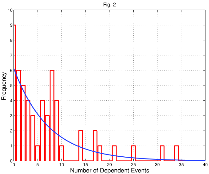
Figure 2:

Red bars – distribution of aftershock numbers $m\geq 4.7$ in the PDE catalog 1977-2007, following $7.2>m_{W}\geq 7.1$ earthquakes in the CMT catalog. The blue line is an approximation of the distribution using the geometric law (Eqs. 5 and 6) with the parameter $\hat{p}=0.1279$, calculated using (26).

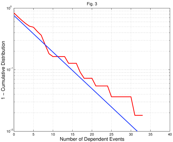
Figure 3:

Red line – survival function (1 - Cumulative distribution) of aftershock numbers $m\geq 4.7$ in the PDE catalog 1977-2007, following $7.2>m_{W}\geq 7.1$ earthquakes in the CMT catalog. The blue line is an approximation of the distribution using the geometric law (Eqs. 5 and 6).

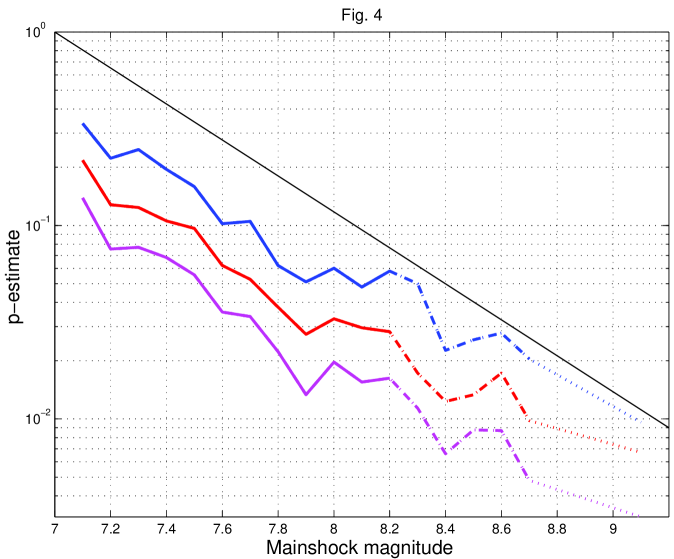
Figure 4:

Dependence of the $\hat{p}$-estimate on mainshock magnitude. The blue line is for $m5.0$ aftershocks during 1-day interval after a mainshock, the red line is for $m4.7$ aftershocks during 1-day interval after a mainshock, and the magenta line is for $m4.7$ aftershocks during a 7-day interval after a mainshock. Solid lines connect data points with more than 3 mainshocks, dashed lines are for a single mainshock, and dotted lines connect the estimate for 2004 $m9.1$ Sumatra earthquake. The thin black line corresponds to $p\propto 10^{-1.5\,m\,\beta}$ (see Eq. 4).

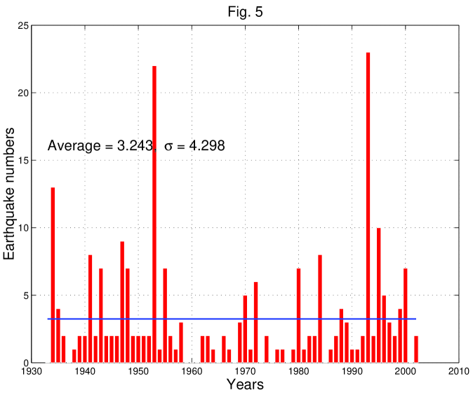
Figure 5:

Annual numbers of earthquakes $m\geq 5.0$ in southern California, 1932-2001.

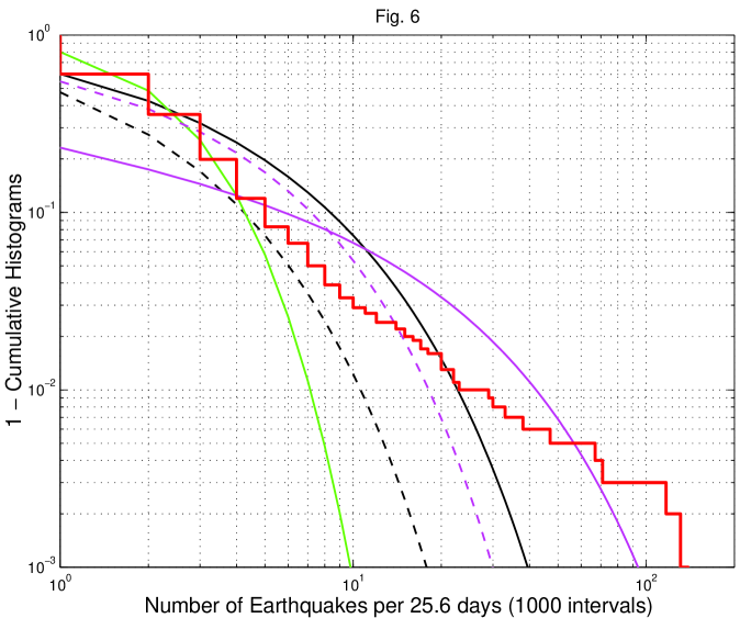
Figure 6:

Survival function (1 - Cumulative distribution) of earthquake numbers for the CIT catalog 1932-2001, $m~{}\geq~{}4.0$. The step-function shows the observed distribution in 25.6 days time intervals (1000 intervals for the whole time period). The green curve is the approximation by the Poisson distribution (14, 38); the magenta solid line is the NBD approximation (Eqs. 15, 18, and 39), with parameters estimated by the MLE method; the magenta dashed curve is the NBD approximation with parameters are estimated by the moment method (see Subsection 2.3); the black dashed line is the approximation by the logarithmic distribution (10); the black solid line is the approximation by the logarithmic law for the zero-truncated distribution.

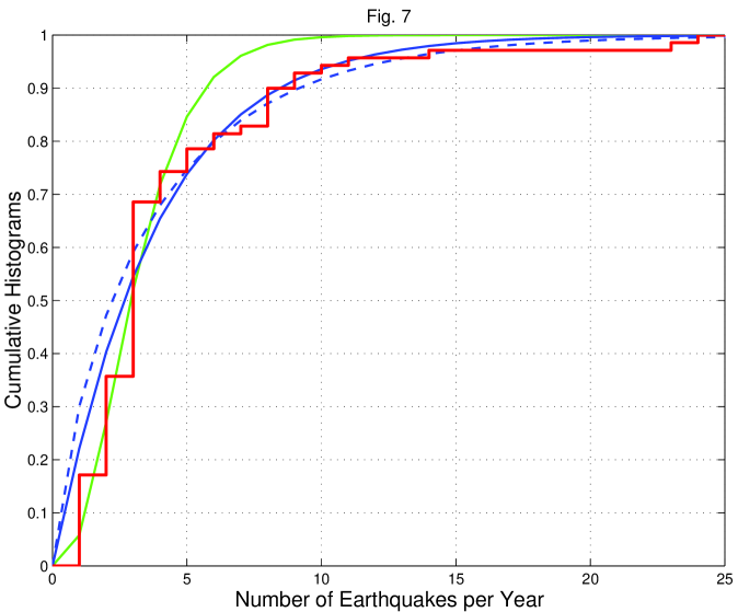
Figure 7:

Cumulative distribution of annual earthquake numbers for the CIT catalog 1932-2001, $m~{}\geq~{}5.0$. The step-function shows the observed distribution, and the solid green curve is the theoretical Poisson distribution (38). Two negative binomial curves (39) are also displayed: for the dashed curve the parameters $\theta$ and $\tau$ are evaluated by the moment method, for the solid curve MLEs are used. The negative binomial curves fit the tails much better than the Poisson does.

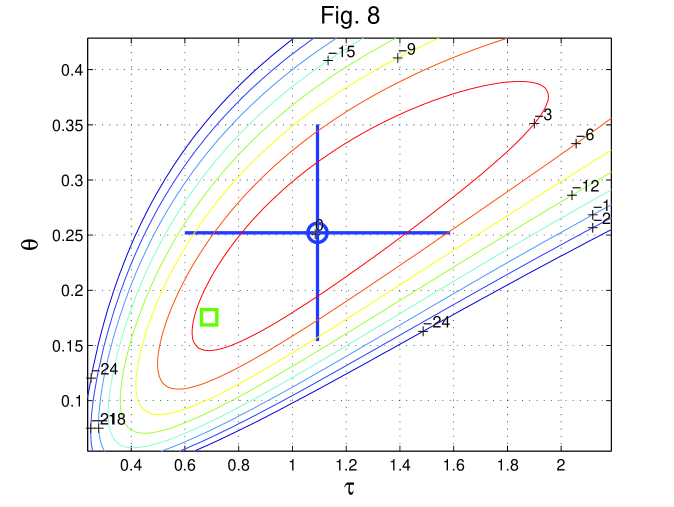
Figure 8:

The log-likelihood function map for the CIT earthquake catalog 1932-2001, $m\geq 5.0$, annual event numbers are analyzed. The standard representation of the NBD (15) is used. The green square is the estimate of $\theta$ and $\tau$ by the moment method, whereas blue circle shows the MLE parameter values. An approximate $95\%$-confidence area, based on asymptotic relations, corresponds to the contour labeled $-3.0$. Two orthogonal line intervals centered at the circle are 95% confidence limits for both parameters, obtained by matlab (Statistics Toolbox). The correlation coefficient $\rho$ between these estimates (also evaluated by matlab) is 0.867.

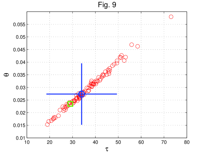
Figure 9:

The standard NBD parameter calculations for PDE earthquake catalog 1969-2007, $m\geq 5.0$, annual event numbers are analyzed. The large green square is the estimate of $\theta$ and $\tau$ by the moment method, whereas large blue circle shows the MLE parameter values: $\tau=33.98\pm 15.42$ and $\theta=0.0274\pm 0.0122$. Two orthogonal line intervals centered at the circle are 95% confidence limits for both parameters. Small circles are simulated parameter estimates, using MLEs. In simulations the parameter estimates for $\theta$ and $\tau$ are also MLEs (see above).

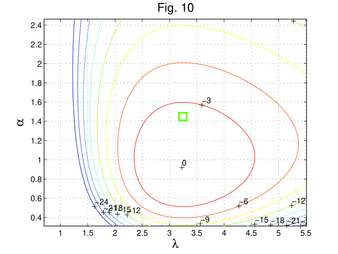
Figure 10:

The log-likelihood function map for CIT earthquake catalog 1932-2001, $m\geq 5.0$, annual event numbers are analyzed. The alternative representation of the NBD (18) is used. The green square is the estimate of $\theta$ and $\lambda$ by the moment method. An approximate $95\%$-confidence interval, based on asymptotic relations, corresponds to the contour labeled $-3.0$.

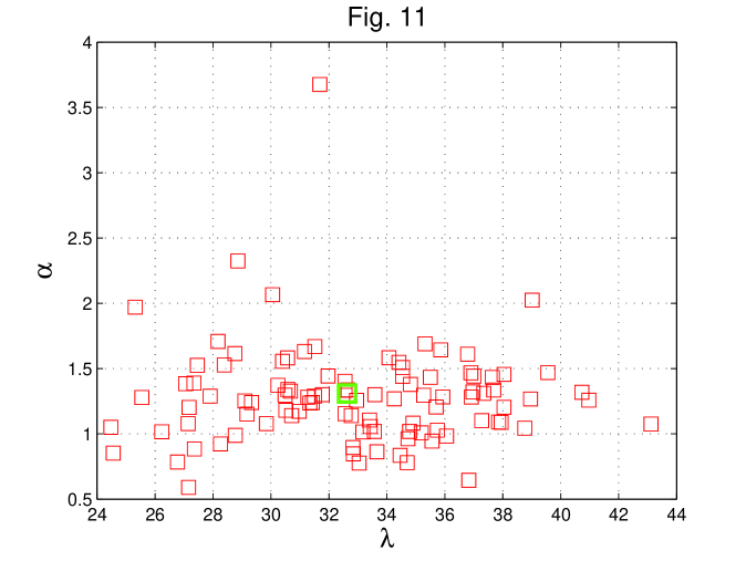
Figure 11:

Simulation results for Caltech earthquake catalog 1932-2001, $m\geq 4.0$, annual event numbers are analyzed. The alternative representation of the NBD (18) is used. The large green square is the estimate of $\alpha$ and $\lambda$ by the moment method for the catalog data. Small squares are simulated parameter estimates, using $\alpha$ and $\lambda$ as input. In these displays the parameters $\alpha$ and $\lambda$ are moment estimates.

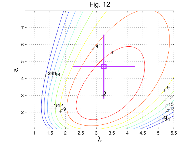
Figure 12:

The likelihood function map for CIT earthquake catalog 1932-2001, $m\geq 5.0$, annual event numbers are analyzed. Evans’ (1953) representation of the NBD (20) is used. The red square is the moment estimate of $a$ and $\lambda$. An approximate $95\%$-confidence interval, based on asymptotic relations, corresponds to the contour labeled $-3.0$. Two orthogonal line intervals centered at the square are 95% confidence limits for both parameters, based on Evans’ (1953) variance formula for moment estimates.

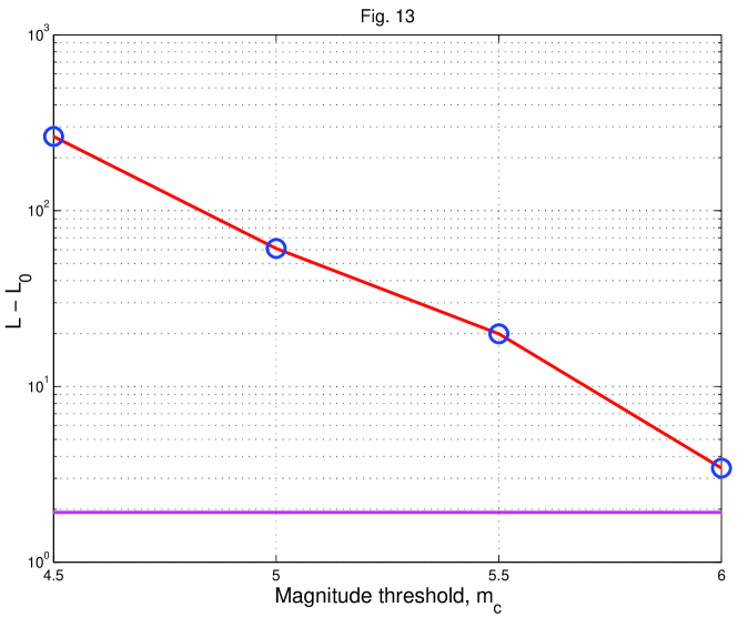
Figure 13:

Dependence of the log-likelihood difference for the NBD and Poisson models of earthquake occurrence on the threshold magnitude. The CIT catalog 1932-2001 is used, annual event numbers are analyzed. The magenta line corresponds to $\ell-\ell_{0}=1.92$; for a higher log-likelihood difference level the Poisson hypothesis should be rejected at the 95% confidence limit.

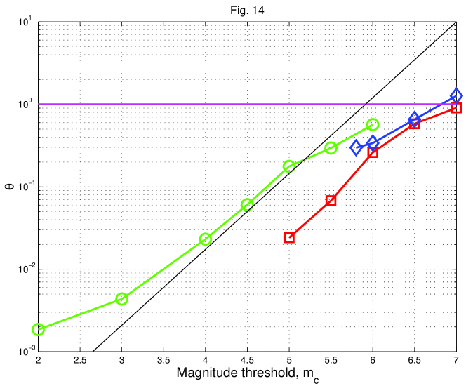
Figure 14:

Dependence of the $\theta$-value for the NBD model (15) of earthquake occurrence on the threshold magnitude. Three catalogs are used: the green curve is for the CIT catalog 1932-2001, the red curve is for the PDE catalog 1969-2007, and the blue curve is for the CMT catalog 1977-2007. The magenta line is $\theta=1.0$, corresponding to the Poisson occurrence. Thin black line corresponds to $\theta\propto 10^{1.5\,m\,\beta}$ (see Eq. 4).

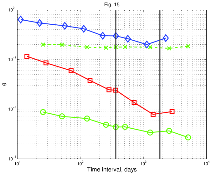
Figure 15:

Dependence of the $\theta$-value for the NBD model (15) of earthquake occurrence on time interval duration ($\Delta T$). Three catalogs are used: the green curve is for the CIT catalog 1932-2001 (circles are for $m3$ earthquakes and crosses for $m5$); the red curve is for the PDE catalog 1969-2007, and the blue curve is for the CMT catalog 1977-2007. Two black vertical lines show 1-year and 5-year intervals.