Quantum spin Hall effect and spin-charge separation in a kagomé lattice

Abstract

A two-dimensional kagomé lattice is theoretically investigated within a simple tight-binding model, which includes the nearest neighbor hopping term and the intrinsic spin-orbit interaction between the next nearest neighbors. By using the topological winding properties of the spin-edge states on the complex-energy Riemann surface, the spin Hall conductance is obtained to be quantized as $-e/2\pi$ ($e/2\pi$) in insulating phases. This result keeps consistent with the numerical linear-response calculation and the Z₂ topological invariance analysis. When the sample boundaries are connected in twist, by which two defects with $\pi$ flux are introduced, we obtain the spin-charge separated solitons at $1/3$ (or $2/3$) filling.

Over the last two decades the topological band insulators (TBIs) have been a subject of great interest in condensed matter field Thouless ; Wenbook . Different from the normal band insulators, the TBIs have a prominent feature, which is the necessary presence of gapless edge states on the sample boundaries Halperin ; Hatsugai . An early TBI model was proposed by Haldane Haldane . Therein it was shown that the gapless edge states result in a remarkable character of TBIs by showing quantum Hall effect in the absence of an external magnetic field. Besides the Haldane model, several other lattice models have also been proposed to be quantum Hall TBIs, which include the two-dimensional (2D) Ohgushi ; Tail ; Wang2 and three-dimensional (3D) Tak spin-chiral kagomé lattices, and the 3D distorted fcc lattice Shindou ; Wang3 . All the quantum Hall TBIs rely on the breaking of time-reversal symmetry (TRS).

Recently, Kane and Mele generalized the spinless Haldane model to a spin one by adding an intrinsic spin-orbit interaction (SOI) Kane1 ; Kane2 . The TRS is conserved in the Kane-Mele model and the gapless spin edge states in this model result in quantum spin Hall effect. These TBIs like the Kane-Mele model keep TRS and are different from the quantum Hall TBIs. Thus call them the quantum spin Hall TBIs. At present the quantum spin Hall TBIs are receiving considerable attention. One impressive example is that only one year later after its theoretical prediction to be a quantum spin Hall TBI in 2006 Bernevig , it was proved in experiment that HgTe is an actual one Koenig .

One special character of the quantum spin Hall TBIs was recently attributed to their spin-charge separated excitations Ran ; Qi in the presence of a $\pi$ flux. This attribution is motivated by the recent advance in studying 2D fractionalized quasiparticles Lee ; Hou , and is a straightforward result when, like what Kane and Mele Kane1 have dealt with Haldane’s TBI, considering spins of the 2D edge soliton. The separate spinon, holon and chargeon obey Bose statistics, and the experimental measurement of these soliton excitations would provide an undoubted verification of the Z₂ topological properties of the quantum spin Hall TBIs. At present, besides the necessity for further studies to gain more insights into the nature of spin-charge separation and its connection to the other topological phenomena, obviously, it is also important to identify and study various model systems that exhibit the phenomenon of spin-charge separation. Motivated by this observation, as well as by the recent attention on the layered metal oxides as possible candidates for the quantum spin Hall TBI Shitade , in this paper, we study the quantum spin Hall effect and construct spin-charge separated edge solitons in a 2D kagomé lattice. Different from the previously studied kagomé TBI Ohgushi ; Tail ; Wang2 ; Tak ; Fuj ; Zhang whearein the presence of ferromagnetic spin chirality breaks TRS, here TRS persists and the quantum spin Hall effect occurs due to the intrinsic SOI. Experimentally, the physical candidates for realizing our studied system might be $5d$ transition metal oxides with layered pyrochlore structure Man ; Singh ; Mat . The argument is that in $5d$ transition metal oxides, both the SOI and the electron correlation become important with the same order of magnitude. As a consequence, at high temparture the correlation-induced magnetic order can be overcome by SOI and the nontrivial topological insulator phase is expected to occur Shitade ; Rag ; Chen ; Kim ; Pesin . The other alternative way to experimentally realize our studied system is by modulating the 2D electron with a periodic potential with kagomé symmetry, as recently demonstrated for artificial graphene Gib . By using the bulk linear-response theory, as well as the topological winding numbers of the spin-edge states on the complex-energy Riemann surface, we obtain the spin Hall conductance (SHC) $\sigma_{xy}^{s}$. The quantized value of $\sigma_{xy}^{s}$ is $-e/2\pi$ ($e/2\pi$) at 1/3 (2/3) filling. Then, we construct spin-charge separated edge solitons by introducing $\pi$ fluxes with a method similar to that in Ref. Lee . The quantum statistics of these solitons is also discussed.

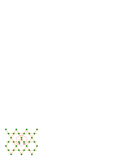
Figure 1: (Color online). Schematic picture of the 2D kagomé lattice. The dashed lines represent the Wigner-Seitz unit cell, which contains three independent sites (A, B, C).

Consider the tight-binding model for independent electrons on a 2D kagomé lattice (Fig. 1). The spin-independent part of the Hamiltonian is given by

$$\mathcal{H}_{0}=t\sum_{\langle ij\rangle\sigma}c_{i\sigma}^{{\dagger}}c_{j\sigma},$$ (1)

where $t_{ij}$=$t$ is the hopping amplitude between the nearest-neighbor link $\langle ij\rangle$ and $c_{i\sigma}^{{\dagger}}$ ($c_{i\sigma}$) is the creation (annihilation) operator of an electron with spin $\sigma$ (up or down) on lattice site $i$. For simplicity, we choose $t$=$-1$ as the energy unit and the distance $a$ between the nearest sites as the length unit throughout this paper.

The Hamiltonian (1) can be diagonalized in the momentum space as

$$\mathcal{H}_{0}=\sum_{\mathbf{k}}\psi_{\mathbf{k}\sigma}^{+}H_{0}(\mathbf{k})\psi_{\mathbf{k}\sigma},$$ (2)

where the electron field operator $\psi_{\mathbf{k}\sigma}$=$(c_{A\mathbf{k}\sigma},c_{B\mathbf{k}\sigma},c_{C\mathbf{k}\sigma})^{\text{T}}$ includes the three lattice sites ($A,B,C$) in the Wigner-Seitz unit cell shown in Fig. 1. $H_{0}(\mathbf{k})$ is a $3\mathtt{\times}3$ spinless matrix given by

$$H_{0}(\mathbf{k})=-t\left(\begin{array}[c]{ccc}0&2\cos\left(\mathbf{k}\mathtt{\cdot}\mathbf{a}_{1}\right)&2\cos\left(\mathbf{k}\mathtt{\cdot}\mathbf{a}_{3}\right)\\ 2\cos\left(\mathbf{k}\mathtt{\cdot}\mathbf{a}_{1}\right)&0&2\cos\left(\mathbf{k}\mathtt{\cdot}\mathbf{a}_{2}\right)\\ 2\cos\left(\mathbf{k}\mathtt{\cdot}\mathbf{a}_{3}\right)&2\cos\left(\mathbf{k}\mathtt{\cdot}\mathbf{a}_{2}\right)&0\end{array}\right),$$ (3)

where $\mathbf{a}_{1}$=$(-1/2,-\sqrt{3}/2)$, $\mathbf{a}_{2}$=$(1,0)$, and $\mathbf{a}_{3}$=$(-1/2,\sqrt{3}/2)$ represent the displacements in a unit cell from A to B site, from B to C site, and from C to A site, respectively. In this notation, the first Brillouin zone (BZ) is a hexagon with the corners of $\mathbf{K}$=$\pm\left(2\pi/3\right)\mathbf{a}_{1}$, $\pm\left(2\pi/3\right)\mathbf{a}_{2}$, $\pm\left(2\pi/3\right)\mathbf{a}_{3}$.

The energy spectrum for spinless Hamiltonian $H_{0}(\mathbf{k})$ is characterized by one dispersionless flat band ($\epsilon_{1\mathbf{k}}^{(0)}$=$2$), which reflects the fact that the 2D kagomé lattice is a line graph of the honeycomb structure Mie , and two dispersive bands, $\epsilon_{2(3)\mathbf{k}}^{(0)}=-1\mathtt{\mp}\sqrt{4b_{\mathbf{k}}-3}$ with $b_{\mathbf{k}}$=$\sum_{i=1}^{3}\cos^{2}\left(\mathbf{k\cdot a}_{i}\right)$. These two dispersive bands touch at the corners (K-points) of the BZ and exhibit Dirac-type energy spectra, $\epsilon_{2(3)\mathbf{k}}^{(0)}\mathtt{=}(-1\mathtt{\mp}\sqrt{3}|\mathbf{k}\mathtt{-}\mathbf{K}|)$, which implies a “particle-hole” symmetry with respect to the Fermi energy $\epsilon_{F}\mathtt{=}-1$. The corresponding eigenstates of $H_{0}(\mathbf{k})$ are given by

$$\left|u_{n\mathbf{k}}^{(0)}\right\rangle=G_{n\mathbf{k}}\left(q_{1\mathbf{k}},q_{2\mathbf{k}},q_{3\mathbf{k}}\right)^{\text{T}},$$ (4)

where the expressions of the components $q_{i\mathbf{k}}$ and the normalized factor $G_{n}(\mathbf{k})$ for each band are given in Table I.

Table 1: The expressions for the coefficients in Eq. (4) with $x_{i}$=$\mathbf{k\mathtt{\cdot}a}_{i}$.

$q_{1k}$	$\ \ \ \ \ \ \ \ \ \ \ \ \ \ \ \ \ \ \frac{1}{2}[\epsilon_{nk}^{(0)2}-4\cos^{2}x_{2}]$
$q_{2k}$	$\ \ \ \ \ \ \ \ \ \ \ \ \ \ \ \ \ \ \epsilon_{nk}^{(0)}\cos x_{1}+2\cos x_{2}\cos x_{3}$
$q_{3k}$	$\ \ \ \ \ \ \ \ \ \ \ \ \ \ \ \ \ \ \epsilon_{nk}^{(0)}\cos x_{3}+2\cos x_{2}\cos x_{1}$
$G_{nk}^{-2}$	$\ \ \ \ \ 2b_{k}\epsilon_{nk}^{(0)2}+[4b_{k}-3\epsilon_{nk}^{(0)2}]\cos^{2}x_{2}+6(b_{k}-1)\epsilon_{nk}^{(0)}\ \$

Then, we introduce the intrinsic SOI term, which, according to the symmetry of the kagomé lattice, takes the form Kane1 ; Guo

$$\mathcal{H}_{\text{SO}}=i\frac{2\lambda_{\text{SO}}}{\sqrt{3}}\sum_{\langle\langle ij\rangle\rangle\sigma_{1}\sigma_{2}}\left(\mathbf{d}_{ij}^{1}\times\mathbf{d}_{ij}^{2}\right)\cdot\mathbf{s}_{\sigma_{1}\sigma_{2}}c_{i\sigma_{1}}^{{\dagger}}c_{j\sigma_{2}}.$$ (5)

Here $\lambda_{\text{SO}}$ represents the SOI strength, $\mathbf{s}$ is the vector of Pauli spin matrices, $i$ and $j$ are next-nearest neighbors, and $\mathbf{d}_{ij}^{1}$ and $\mathbf{d}_{ij}^{2}$ are the vectors along the two bonds that connect $i$ to $j$. Taking the Fourier transform, we have

$$\mathcal{H}_{\text{SO}}\mathtt{=}\sum_{\mathbf{k}\sigma}\psi_{\mathbf{k}\sigma}^{+}H_{\text{SO}}(\mathbf{k})\psi_{\mathbf{k}\sigma}$$

with

$$H_{\text{SO}}(\mathbf{k})=\pm 2\lambda_{\text{SO}}\left(\begin{array}[c]{ccc}0&i\cos(\mathbf{k}\mathtt{\cdot}\mathbf{b}_{1})&-i\cos(\mathbf{k}\mathtt{\cdot}\mathbf{b}_{3})\\ -i\cos(\mathbf{k}\mathtt{\cdot}\mathbf{b}_{1})&0&i\cos(\mathbf{k}\mathtt{\cdot}\mathbf{b}_{2})\\ i\cos(\mathbf{k}\mathtt{\cdot}\mathbf{b}_{3})&-i\cos(\mathbf{k}\mathtt{\cdot}\mathbf{b}_{2})&0\end{array}\right),$$ (6)

where $\mathbf{b}_{1}$=$\mathbf{a}_{3}-\mathbf{a}_{2}$, $\mathbf{b}_{2}$=$\mathbf{a}_{1}-\mathbf{a}_{3}$, $\mathbf{b}_{3}$=$\mathbf{a}_{2}-\mathbf{a}_{1}$, and the $+$($-$) sign refers to spin up (down) electrons.

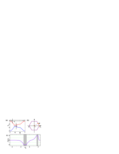
Figure 2: (Color online). (a) Energy spectrum (solid curves) of the 2D kagomé lattice along the high-symmetry lines in the BZ with intrinsic spin-orbit couplings $\lambda_{\text{SO}}$=$0.1t$. There are two band gaps appearing with gap width $\Delta$ and $\delta$. For comparison, we also draw the energy spectrum without intrinsic spin-orbit couplings (dotted lines). (b) The corresponding BZ of the 2D kagomé lattice. (c) The SHC $\sigma_{xy}^{s}$ as a function of the Fermi energy $\epsilon_{F}$. The shaded areas correspond to the bulk gaps.

Inclusion of the intrinsic SOI in the Hamiltonian makes the appearance of the eigenstates $\left|u_{n\mathbf{k}}\right\rangle$ and eigenenergies $\epsilon_{n\mathbf{k}}$ very tedious with exception at some high-symmetry $\mathbf{k}$ points. Instead of writing their explicit forms, here we show in Fig. 2(a) (solid curves) the numerically calculated energy spectrum for the total Hamiltonian $\mathcal{H}\mathtt{=}\mathcal{H}_{0}\mathtt{+}\mathcal{H}_{\text{SO}}$ along the high-symmetry lines ($\mathbf{\Gamma}\mathtt{\rightarrow}\mathbf{K}$, $\mathbf{K}\mathtt{\rightarrow}\mathbf{M}$, and $\mathbf{M}\mathtt{\rightarrow}\mathbf{\Gamma}$) in the BZ. The SOI coefficient is chosen to be $\lambda_{\text{SO}}$=$0.1t$. For comparison we also plot in Fig. 2(a) (dashed curves) the energy spectrum in the absence of SOI ($\lambda_{\text{SO}}$=$0$). One can see that while the spin degeneracy is not lifted by the presence of the intrinsic SOI, nevertheless, the Dirac contacts of the lower and middle bands at the $\mathbf{K}$ point are removed and a gap of amplitude $\Delta$=$4\sqrt{3}|\lambda_{\text{SO}}|$ opens between these two bands. The amplitude of this gap turns out to be $\Delta$=$4\sqrt{3}|\lambda_{\text{SO}}|$. Similarly, the original contact at the $\mathbf{\Gamma}$ point between the middle and upper (flat) bands is also lifted by the presence of SOI and a gap with amplitude $\delta$ is opened. However, this gap is an indirect one, i.e., the middle-band maximum and upper-band minimum are not at the same $k$-point.

To see the behavior of the system in the insulating state, we have calculated the SHC using the following Kubo formula Sinova

$$\sigma_{xy}^{s} =-e\hslash\sum_{n\neq n^{\prime},\mathbf{k}}\left[f\left(\epsilon_{n\mathbf{k}}\right)-f\left(\epsilon_{n^{\prime}\mathbf{k}}\right)\right]$$ (7)

$$\times\frac{\operatorname{Im}\langle u_{n\mathbf{k}}|\frac{1}{2}\left\{\hat{v}_{x},\hat{s}_{z}\right\}|u_{n^{\prime}\mathbf{k}}\rangle\langle u_{n^{\prime}\mathbf{k}}|\hat{v}_{y}|u_{n\mathbf{k}}\rangle}{\left(\epsilon_{n\mathbf{k}}-\epsilon_{n^{\prime}\mathbf{k}}\right)^{2}+\eta^{2}},$$

where $\mathbf{\hat{v}}\left(\mathbf{k}\right)$=$\partial H(\mathbf{k})/\hslash\partial\mathbf{k}$ and $H(\mathbf{k})$=$H_{0}(\mathbf{k})+H_{\text{SO}}(\mathbf{k})$. The calculated result at zero temperature is shown in Fig. 2(c) by varying the Fermi energy $\epsilon_{F}$ with the SOI coefficient $\lambda_{\text{SO}}$=$0.1t$. From Fig. 2(c), one can see that initially the SHC $\sigma_{xy}^{s}$ decreases as the filling factor of the (spin-degenerate) lower band increases, arriving at the minimum value $-(e/2\pi)$ at $\epsilon_{F}$=$-1.35$ (=$-1\mathtt{-}\Delta/2$), a value corresponding to the top of the lower band. Then, as the Fermi energy $\epsilon_{F}$ continues to vary in the first gap region (shaded area wherein $-1.35\mathtt{\leqslant}\epsilon_{F}\mathtt{\leqslant}-0.65$), the SHC keeps this minimum value unchanged. As shown in the following discussion, this quantized SHC can be understood by the Z₂-valued topological invariant associated with this quantum spin Hall phase Kane2 . When the Fermi energy increases to touch the bottom of the middle band at $\epsilon_{F}$=$-0.65$(=$-1+\Delta/2$), then the SHC suddenly switches up and rapidly increases when the Fermi energy goes through the middle two bands. When $\epsilon_{F}$ increases to be at the top of the middle two bands ($\epsilon_{F}$=$1.65$), $\sigma_{xy}^{s}$ arrives at the maximum value $e/2\pi$. Then as the Fermi energy $\epsilon_{F}$ continues to vary in the second gap region (shaded area $1.65\mathtt{\leqslant}\epsilon_{F}\mathtt{\leqslant}2$), the SHC $\sigma_{xy}^{s}$ keeps this maximum value unchanged. When the Fermi energy increases to touch the bottom of the upper band at $\epsilon_{F}$=$2$, the SHC then suddenly switches down and rapidly decreases when the Fermi energy goes through the upper band. Finally the SHC $\sigma_{xy}^{s}$ decreases to disappear when the three spin-degenerate bulk bands are all fully occupied.

Topologically, the quantum spin Hall insulating state at $1/3$ or $2/3$ filling can be seen by calculating a selective Z₂-valued invariant $\nu$ Kane2 , which is related to the parity eigenvalues $\xi_{2m}(\Gamma_{i})$ of the $2m$-th occupied energy band at the four time-reversal-invariant momenta $\Gamma_{i}$ Fu . Very recently, Guo and Franz Guo have numerically calculated the eigenstate of $\mathcal{H}_{\Gamma_{i}}$ and they found that three $\xi$’s are positive and one is negative. Although which of the four $\xi$’s is negative depends on the choice of the inversion center, the product $\Pi_{i}\xi(\Gamma_{i})$=$(-1)^{\nu}$ is independent of this choice and determines the nontrivial Z₂ invariant $\nu$=$1$. That confirms the kagomé lattice system to be a quantum spin Hall TBI at $1/3$ (or $2/3$) filling.

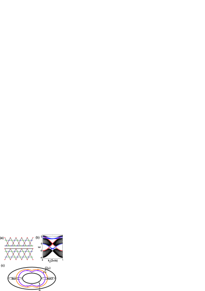
Figure 3: (Color online). (a) Sketch of the 2D kagomé lattice strip with two edges along the $y$ direction. The red, blue, and green dots are used to distinguish the independent sites A, B, and C, respectively. (b) Energy spectrum of the kagomé lattice strip ($N_{y}$=$40$) with the Hamiltonian $\mathcal{H}$=$\mathcal{H}_{0}+\mathcal{H}_{\text{SO}}$. The spin-orbit coupling strength is set as $\lambda_{\text{SO}}$=$0.1t$. The red and blue lines represent the edge states localized at the down and up edges of the system, respectively. And the circle and triangle label the up and down spins, respectively. (c) The Riemann surface of the Bloch function corresponding to $1/3$ filling. The purple and orange curves correspond to spin-up and spin-down channels, respectively.

On the other hand, the topological aspect of the quantized spin Hall phase can be distinguished by the difference between the winding numbers of the spin-up and spin-down edge states across the holes of the complex-energy Riemann surface, $I_{s}$=$I_{\uparrow}-I_{\downarrow}$ Wang5 . The SHC is then given by $\sigma_{xy}^{s}$=$I_{s}\left(e/4\pi\right)$. Using this topological index $I_{s}$ we have investigated the quantum spin Hall effect in the Kane-Mele graphene model Wang5 . For the present kagomé lattice model we can also study the quantum spin Hall effect in terms of this topological winding index. For this purpose, let us first numerically diagonalize the total Hamiltonian $\mathcal{H}$ using the strip geometry. For convenience and without loss of generality, we suppose the system has two edges in the $y$ direction while keeping infinite in the $x$ direction [see Fig. 3(a)]. The number of sites $A$ (or $B,C$) in the $y$ direction is chosen to be $N_{y}$=$40$. The calculated energy spectrum is drawn in Fig. 3(b). From this figure one can clearly see that there are spin edge states occurring in each energy gap. These gapless edge states in the truncated kagomé lattice are topologically stable against random-potential perturbation, provided that the perturbation is small compared to the bulk gaps. We have numerically confirmed this fact. The Riemann surface of Bloch function is plotted in Fig. 3(c) for $1/3$ filling. According to Ref. Wang5 , the winding number of spin-up (spin-down) edge state in the lower gap is $I_{\uparrow}$=$-1$ ($I_{\downarrow}$=$1$), which gives $I_{s}$=$-2$ at $1/3$ filling. That means the SHC in this phase is quantized as $\sigma_{xy}^{s}$=$-(e/2\pi)$. The Riemann surface of Bloch function at $2/3$ filling are the same as that at $1/3$ filling, except that the directions of the curves corresponding to different spin channels are inverse. So the winding number of spin-up (spin-down) edge state in the upper gap is $I_{\uparrow}$=$1$ ($I_{\downarrow}$=$-1$), which gives $I_{s}$=$2$. The corresponding SHC at $2/3$ filling is then quantized as $\sigma_{xy}^{s}$=$e/2\pi$. These conclusions are consistent with those calculated by using the Kubo formula (7) [see Fig. 2(c)]. Note that although the non-trivial Z₂ invariant $\nu$=$1$ in the bulk analysis can confirm the quantum spin Hall TBI phase, it does not provide the information on the sign of the SHC. In contrast, our winding-number analysis can resolve this sign at different fillings (i.e., $\sigma_{xy}^{s}$=$\mp(e/2\pi)$ at $1/3$ and $2/3$ filling, respectively).

The topological properties of the system in the insulating state are stable even when the Rashba SOI is considered. To clearly see this fact, we numerically calculated the SHC $\sigma_{xy}^{s}$ with the Kubo formula (7) when the total Hamiltonian includes the Rashba SOI Liu

$$\mathcal{H}_{R}=i\frac{\lambda_{R}}{\hslash}\sum_{\langle ij\rangle\sigma_{1}\sigma_{2}}c_{i\sigma_{1}}^{{\dagger}}(\mathbf{s}\times\mathbf{\hat{d}}_{ij})_{z}c_{j\sigma_{2}},$$ (8)

where $\lambda_{R}$ is the Rashba coefficient and $\mathbf{\hat{d}}_{ij}$ is a vector along the bond the electron traverses going from site $j$ to $i$. The calculated SHC is drawn in Fig. 4 for different values of $\lambda_{R}$. Clearly, one can see that the amplitude of SHC in the insulating phase keeps $e/2\pi$ unchanged when the Rashba SOI strength $0\mathtt{\leqslant}\lambda_{R}/t\mathtt{<}0$.$1$. When the Rashba SOI is sufficiently large (for example $\lambda_{R}$=$0$.$2t$), the amplitude of SHC will depart little from the quantized value. However, the topology of this insulating state keeps unchanged, unless the bulk gaps disappear.

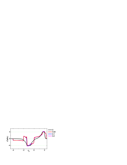
Figure 4: (Color online). The SHC as a function of the Fermi energy $\epsilon_{F}$ with different values of the Rashba coefficient. The black, red, blue, and pink lines correspond to $\lambda_{R}$=$0$, $0.02t$, $0.1t$, and $0.2t$, respectively. The intrinsic SOI strength is set as $\lambda_{\text{SO}}$=$0.1t$.

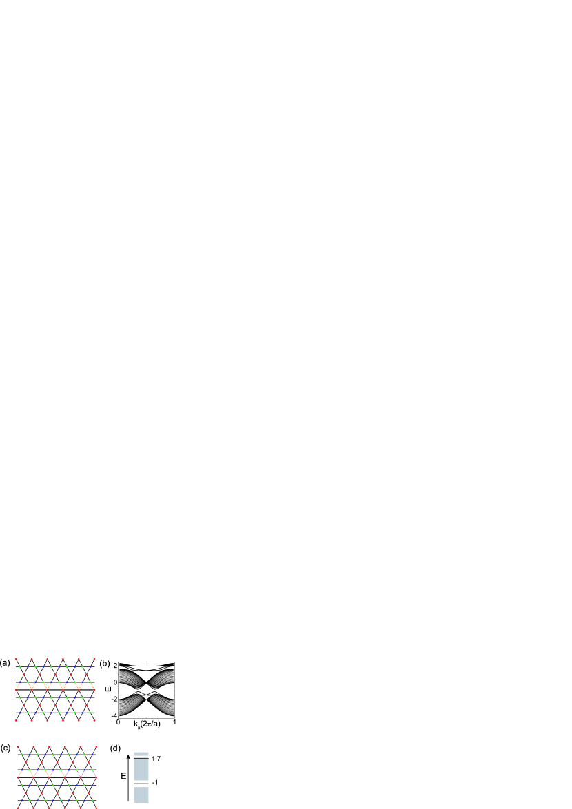
Figure 5: (Color online). (a) Two edges of the 2D kagomé lattice are reconnected with weaker bonds (orange dotted lines) and its corresponding energy spectrum (b). (c) The restored bonds have a sign reversal along the right half bonds (violet dotted lines) and its corresponding energy spectrum (d). In these figures, the system size is set as $N_{y}$=$40$ and the spin-orbit coupling $\lambda_{\text{SO}}$=$0.1t$. The bonds connected two edges are set as $0.25$ times of other ones.

In the following let us consider the spin-charge separation in the 2D kagomé lattice. If we reconnect the two edges of the kagomé lattice shown in Fig. 3(a) with weaker bonds, two small gaps then reappear in the edge spectrum [see Figs. 5(a) and (b)]. Topological excitations (edge solitons) are created by reversing the sign of the reconnected bonds along the right half row [see Fig. 5(c)]. In this manner two defects with $\pi$ flux are introduced in the present kagomé lattice. As a result, four degenerate in-gap spin states localized around these two defects are formed in each bulk gap [see Figs. 5(d)]. The corresponding energies of these in-gap states are $\epsilon$=$-t$ and $1.7t$, respectively. Note that in the square lattice version of the Kane-Mele model Ran , the in-gap modes are precisely at zero energy, while in the present kagomé lattice model the in-gap modes are no longer at zero energy. Here, we would like to point out that the zero level discussed in a large amount of previous studies is a result of particle-hole symmetry. Its role in leading to fermion number fractionalization was initially found by Jackiw and Rebbi Jack , and then stressed in various insulating systems Su1980 ; Lee ; Hou ; Ran ; Qi ; Weeks . In this case, a simple physical picture of fractional charge of $e/2$ around the defect is ready to obtain by the combined fact that (i) under particle-hole symmetry the relative charge density $\rho$ on the soliton and the chemical potential $\mu$ satisfy $\rho(\mu)$=$\mathtt{-}\rho(-\mu)$, and (ii) when $\mu$ is in the bulk gap, the only difference between $\rho(\mu)$ and $\rho(-\mu)$ is the filling of the zero modes localized at the two defects. In the present 2D kagomé lattice, on the other hand, the system has no particle-hole symmetry and thus no zero mode. In this case, although we cannot resort to the above simple physical picture, the presence of soliton-antisoliton doublet (quadruplet when spin included) in each bulk gap in Fig. 5(d) still guarantees the occurrence of fractionalized excitations.

At 1/3 or 2/3 filling, occupation (unoccupation) of these in-gap modes leads to an excess (deficit) of $1/2$ fermion number per spin and per defect Zhang . Four different types of solitons with the following quantum numbers are obtained when these in-gap modes are occupied by different ways: the chargeon $f_{+(1/2)\uparrow,+(1/2)\downarrow}$ (charge $-e$, $S_{z}$=$0$); the holon $f_{-(1/2)\uparrow,-(1/2)\downarrow}$ (charge $e$, $S_{z}$=$0$); the two spinons $f_{+(1/2)\uparrow,-(1/2)\downarrow}$ (charge $0$, $S_{z}$=$\frac{\hslash}{2}$) and $f_{-(1/2)\uparrow,+(1/2)\downarrow}$ (charge $0$, $S_{z}$=$-\frac{\hslash}{2}$). Here the subscript $+$ ($-$) represents that the in-gap mode is filled (empty) and $\uparrow$ ($\downarrow$) labels the spin mode. For example, $f_{+(1/2)\uparrow,-(1/2)\downarrow}$ means that the up-spin mode is filled and the down-spin mode is empty. For further illustration, the charge-density distribution for the chargeon $f_{+(1/2)\uparrow,+(1/2)\downarrow}$ is calculated and shown in Fig. 6(a), while the spin-density distribution for the spinon $f_{+(1/2)\uparrow,-(1/2)\downarrow}$ is plotted in 6(b). Here, we use a $24\mathtt{\times}24$ lattice for calculation.

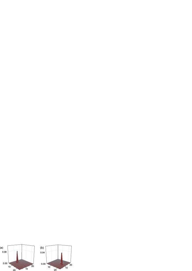
Figure 6: (Color online). (a) The charge density of a chargeon state and (b) the spin density of a spinon on a $24\times 24$ lattice with periodic boundary condition. The chargon at coordinate ($6$, $6$) is $f_{+(1/2)\uparrow,+(1/2)\downarrow}$, it has charge $-e$ and spin $S_{z}$=$0$. The spinon at coordinate ($18$, $18$) is $f_{+(1/2)\uparrow,-(1/2)\downarrow}$, it has charge $0$ and spin $S_{z}$=$\hslash/2$.

The quantum statistics of these spin-charge separated solitons can be readily seen by using anyon fusion argument Weeks ; Ran , which is based on the observation that the bound states of fractional excitation acquire non-trivial Berry phases on adiabatic exchange. Since the spin-up and spin-down bands in the present case decouple, so without loss of generality, let us consider a bound state of two identical spin-up solitons $f_{(1/2)\uparrow}$ (or $f_{-(1/2)\uparrow}$), which carries charge $-e$ ($e$) and flux $2\pi\mathtt{\sim}0$ thus is a fermion. According to the anyon fusion rule, which states that the exchange phase $\Theta$ of a particle formed by combining $n$ identical anyons with exchange phase $\theta$ is $\Theta$=$n^{2}\theta$, one easily obtains that the exchange phase between two identical solitons $f_{(1/2)\uparrow}$ ($f_{-(1/2)\uparrow}$) should be $1/4$ that of fermions, i.e., $\theta(f_{(1/2)\uparrow},f_{(1/2)\uparrow})$ (or $\theta(f_{-(1/2)\uparrow},f_{-(1/2)\uparrow}$)=$\pm\pi/4$. Next let us consider a bound state of an $f_{(1/2)\uparrow}$ and $f_{-(1/2)\uparrow}$ soliton, which carries charge $0$ and should be a boson. Then the exchange phase between solitons $f_{(1/2)\uparrow}$ and $f_{-(1/2)\uparrow}$ is given by $\theta(f_{(1/2)\uparrow},f_{-(1/2)\uparrow})$=$\mp\pi/4$. Since the spin-down band is the Hermitian conjugate of the spin-up band, one obtains $\theta(f_{\alpha_{1}\downarrow},f_{\alpha_{2}\downarrow})$=$-\theta(f_{\alpha_{1}\uparrow},f_{\alpha_{2}\uparrow})$. Substituting these results into the formula calculating the exchange phase between spin-charge separated solitons $\theta(f_{\alpha_{1}\uparrow\beta_{1}\downarrow},f_{\alpha_{2}\uparrow\beta_{2}\downarrow})$=$\theta(f_{\alpha_{1}\uparrow},f_{\alpha_{2}\uparrow})$+$\theta(f_{\beta_{1}\downarrow},f_{\beta_{2}\downarrow})$, one immediately concludes that the spinons, holon, and chargeon are all bosons. However, each spinon has nontrivial mutual exchange phase $\pi$ with the chargeon and holon.

Before ending this paper, we would like to point out that there are other ways for creating the spin-charge separated solitons in the kagomé lattice. For example, by trimerizing the kagomé lattice Guo , like the 1D way proposed by Su and Schrieffer Su , the excitations of possessing fractional charge $\pm e/3$ or $\pm 2e/3$ in two spacial dimensions can be realized. To make this point more clear, now we construct a trimerized pattern of the kagomé lattice by introducing an appropriate bond distortion as shown in Fig. 7(a). The tight-binding Hamiltonian describing this trimerized kagomé lattice is generally written as $\mathcal{H}_{0}=\sum_{\langle ij\rangle}t_{ij}c_{i}^{{\dagger}}c_{j}$, where the hopping amplitude $t_{ij}$ are different for different nearest-neighbor link $\langle ij\rangle$ when the distortion is introduced. For simplicity and without loss of generality, we set in Fig. 7(a) the hopping term along the thick (thin) bonds as $t+\eta$ ($t-\eta$), where $|\eta|$ depicts the distortion amplitude, which is smaller than the undistorted hopping amplitude $|t|$. In this case, the unit cell now becomes larger and contains $9$ sites [see the dashed lines in Fig. 7(a)]. Clearly, there are three different phases corresponding to the ground state (denoted by A, B, and C, respectively). The corresponding spectrum of this distorted kagomé lattice (A, B, or C) with infinite size is drawn in Fig. 7(c). When the system is finite, i.e., it has two boundaries along one direction (say, the $x$ direction), there are edge states appearing in the bulk gaps [see the red thick lines in the spectrum drawn in Fig. 7(d)]. For comparison, we also plot in Fig. 7(b) the spectrum of the 2D perfect undistorted kagomé lattice. In this case the 2D kagomé lattice system has no bulk gaps. Two facts should be noted. One is that the bulk gaps appearing in Figs. 7(c) and 7(d) now result from the distortion. The other is that the in-gap edge states in Fig. 7(d) do not connect the neighboring two bulk bands. According to the winding properties of the edge states Hatsugai ; Wang5 , one knows that the insulating phase risen from the distortion is topologically trivial. That means the Hall conductance is zero when the Fermi energy lies in the bulk gaps. This point has been validated by the numerical calculation with the linear-response formula Sinova .

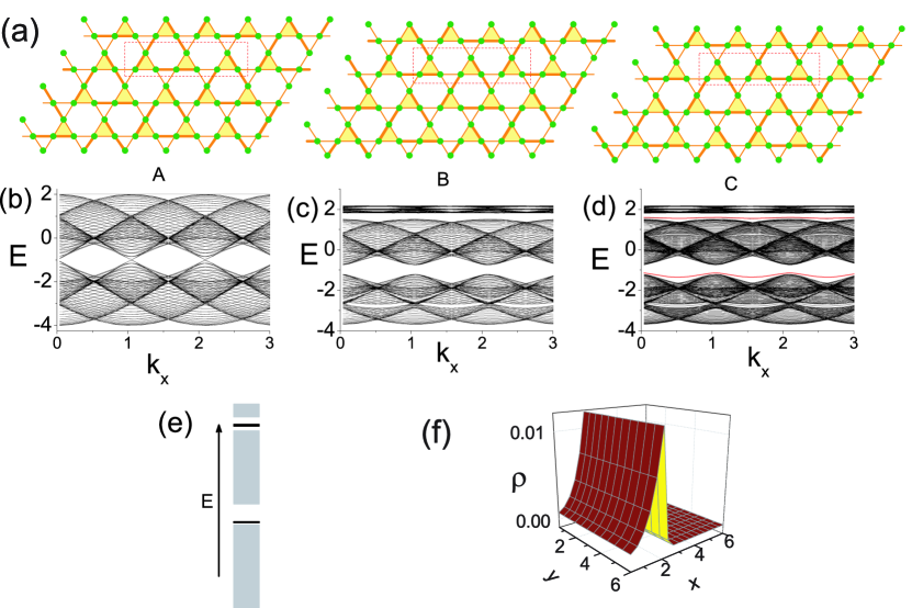
Figure 7: (Color online). (a) Schematic pictures of the three degenerated ground states of a trimerized 2D distorted kagomé lattice. The hopping amplitude along the thick (thin) lines is set as $t+\eta$ ($t-\eta$), where $t$=$-1$ is set as energy unit and $\eta$=$0.25t$. The dashed lines represent the unit cell, which contains $9$ lattice sites. The corresponding energy spectrums are shown in (c) (without boundary) and (d) (with boundary), respectively. The thick lines in (d) represent the edge states. The energy spectrum of the undistorted 2D kagomé lattice ($\eta$=$0$) is drawn in (b). (e) Energy spectrum of the 2D kagomé lattice with kink I. The gray shaded regions represent the bulk bands and the thick black lines represent the excitation energies. (f) The charge density of a fractional chargeon state on a trimerized kagome lattice composed by $36$ units. The chargeon at $x$=$2$ line has charge $-2e/3$ and spin $S_{z}$=$0$.

We can now study the structure of kinks connecting different phases. Similar to the case of one spatial dimension Su , we distinguish two classes of kinks: type I, which leads from A to B, B to C, or C to A as one moves from left to right; and type II, which leads from A to C, C to B, or B to A as one moves along the same direction. Fig. 7(e) plots the energy spectrum of the trimerized kagomé lattice with kink I (or with kink II) by using $1296$ sites. Every phase has $6\times 8$ units and in each unit there are $9$ independent sites. For numerical calculation, we set $t$=$-1$ and the distortion $\eta$=$0.25t$. From Fig. 7(e) one can clearly observe that there are excitation energies appearing in the bulk gaps. In this case, in the lower gap there are $9$ excitation energies while in the higher gap there are $48$ ones. These excitations are localized around the kinks, which is shown in Fig. 7(f). Every kink has fractional charge $-e/3$. That means we have realized the excitations possessing fractional charge $-e/3$ in the trimerized kagomé lattice. When we numerically increase the system size along the $y$ axis, the number of the excitation energies is found to increase in proportion to the system size. In the infinite limit, an excitation band eventually forms in the bulk gap. However, when we increase the size along the $x$ axis, the number of the excitations keeps unchanged. When the spin freedom is considered, one can obtain the spin-charge separated excitations at $1/3$ (or $2/3$) filling. For example, in a small system with $6\times 6$ units, there are $4$ double-degenerate excitation states lying in the lower gap, one half is contributed from the lower bands and one half from the middle one. According to the different occupation ways, the spin-charge separated excitations with fractional quantum numbers, chargeon $\pm 2e/3$, as well as other excitations with fractional charge $\pm e/3$ and spin $\pm\hslash/2$, are obtained.

In summary, we have theoretically studied quantum spin Hall effect and spin-charge separation in a 2D kagomé lattice. By using the topological winding numbers of the spin edge states on the complex-energy Riemann surface, we have obtained that the SHC is quantized as $\pm(e/2\pi)$ when the system is in the insulating phases, which is consistent with the Z₂ topological invariant analysis and the numerical linear-response calculation. Furthermore, we have constructed the spin-charge separated solitons in the kagomé lattice by connecting the system’s boundaries in twist. The quantum statistics of these solitons has also been discussed.

This work was supported by NSFC under Grants No. 10604010, No. 10904005, and No. 60776063, and by the National Basic Research Program of China (973 Program) under Grant No. 2009CB929103.

References

- (1) D. J. Thouless, M. Kohmoto, M. P. Nightingale, and M. den Nijs, Phys. Rev. Lett. 49, 405 (1982).
- (2) X.-G. Wen, Quantum Field Theory of Many-Body Systems (Oxford University Press, New York, 2004).
- (3) B. I. Halperin, Phys. Rev. B 25, 2185 (1982).
- (4) Y. Hatsugai, Phys. Rev. Lett. 71, 3697 (1993).
- (5) F. D. M. Haldane, Phys. Rev. Lett. 61, 2015 (1988).
- (6) K. Ohgushi, S. Marakami, and N. Nagaosa, Phys. Rev. B 62, 6065(R) (2000).
- (7) M. Taillefumier, B. Canals, C. Lacroix, V. K. Dugaev, and P. Bruno, Phys. Rev. B 74, 085105 (2006).
- (8) Z. Wang and P. Zhang, Phys. Rev. B 76, 064406 (2007); Phys. Rev. B 77, 125119 (2008).
- (9) T. Tomizawa and H. Kontani, Phys. Rev. B 80, 100401(R) (2009).
- (10) R. Shindou and N. Nagaosa, Phys. Rev. Lett. 87, 116801 (2001).
- (11) Z. Wang, P. Zhang, and J. Shi, Phys. Rev. B 76, 094406 (2007).
- (12) C. L. Kane and E. J. Mele, Phys. Rev. Lett. 95, 226801 (2005).
- (13) C. L. Kane and E. J. Mele, Phys. Rev. Lett. 95, 146802 (2005).
- (14) B. A. Bernevig, T. L. Hughes, and S.-C. Zhang, Science 314, 1757 (2006).
- (15) M. Koenig, S. Wiedmann, Christoph Brüne, A. Roth, H. Buhmann, L. W. Molenkamp, X.-L. Qi, and S.-C. Zhang, Science 318, 766 (2007).
- (16) Y. Ran, A. Vishwanath, and D.-H. Lee, Phys. Rev. Lett. 101, 086801 (2008).
- (17) X.-L. Qi and S.-C. Zhang, Phys. Rev. Lett. 101, 086802 (2008).
- (18) D.-H. Lee, G.-M. Zhang, and T. Xiang, Phys. Rev. Lett. 99, 196805 (2007).
- (19) C.-Y. Hou, C. Chamon, and C. Mudry, Phys. Rev. Lett. 98, 186809 (2007).
- (20) A. Shitade, H. Katsura, J. Kuneš, X.-L. Qi, S.-C. Zhang, and N. Nagaosa, Phys. Rev. Lett. 102, 256403 (2009).
- (21) S. Fujimoto, Phys. Rev. Lett. 103, 047203 (2009).
- (22) P. Zhang, Z. Wang, N. Hao, and W. Zhang (unpublished).
- (23) D. Mandrus et al., Phys. Rev. B 63, 195104 (2001).
- (24) D. J. Singh, P. Blaha, K. Schwarz, and J. O. Sofo, Phys. Rev. B 65, 155109 (2002).
- (25) K. Matsuhira et al., J. Phys. Soc. Jpn. 76, 043706 (2007).
- (26) S. Raghu, X.-L. Qi, C. Honerkkamp, and S.-C. Zhang, Phys. Rev. Lett. 100, 156401 (2008).
- (27) G. Chen and L. Balents, Phys. Rev. B 78, 094403 (2008).
- (28) B. J. Kim, et al., Science 323, 1329 (2009).
- (29) D. A. Pesin and L. Balents, arXiv:0907.2962.
- (30) M. Gibertini et al., arXiv:0904.4191.
- (31) Z. Wang, N. Hao, and P. Zhang, Phys. Rev. B 80, 115420 (2009).
- (32) A. Mielke, J. Phys. A 24, L73 (1991); 24, 3311 (1991); 25, 4335 (1992).
- (33) H.-M. Guo and M. Franz, Phys. Rev. B 80, 113102 (2009).
- (34) J. Sinova, D. Culcer, Q. Niu, N. A. Sinitsyn, T. Jungwirth, and A. H. MacDonald, Phys. Rev. Lett. 92, 126603 (2004).
- (35) L. Fu and C. L. Kane, Phys. Rev. B 76, 045302 (2007).
- (36) G. Liu, P. Zhang, Z. Wang, and S.-S. Li, Phys. Rev. B 79, 035323 (2009).
- (37) R. Jackiw and C. Rebbi, Phys. Rev. D 13, 3398 (1976).
- (38) W. P. Su, J. R. Schrieffer and A. J. Heeger, Phys. Rev. B 22, 2099 (1980).
- (39) C. Weaks, G. Rosenberg, B. Seradjeh and M. Franz, Nature Phys. 3, 796 (2007).
- (40) W. P. Su and J. R. Schrieffer, Phys. Rev. Lett. 46, 738 (1981).