Near-IR spectra of IPHAS extremely red Galactic AGB stars

Abstract

We present a library of 139 near-IR spectra of cool asymptotic giant branch stars that will be useful for comparison with theoretical model atmosphere calculations and for modeling the integrated emission from intermediate-age stellar populations. The source list was selected from the “extremely red” region of the INT Photometric H$\alpha$ Survey (IPHAS) colour-colour plane that is overwhelmingly dominated by very late-type stars. The spectral library also includes a large fraction of S-type and carbon stars. We present a number of spectral classification sequences highlighting the various molecular features identified and discuss a number of rare features with uncertain identifications in the literature. With its focus on particularly cool photospheres this catalogue serves as a companion to recent spectroscopic atlases of MK standards in the near-IR. Finally the relationship between IPHAS $(r^{\prime}-i^{\prime})$ and $(r^{\prime}-$H$\alpha)$ colours and spectroscopically determined properties is discussed and a strong correlation between $(r^{\prime}-$H$\alpha)$ colour and the C/O abundance index for S-type and carbon stars is noted. This relation has the potential to separate O-rich, S-type and carbon stars in the Galaxy based on their photometry alone.

1 Introduction

Asymptotic giant branch (AGB) stars represent one of the last evolutionary stages passed through by all intermediate mass stars ($0.8<$ M/M${}_{\odot}<8.0$) and are responsible for large amounts of processed material returned to the interstellar medium (ISM). Their cool extended atmospheres and winds are prime sites for the development of molecular chemistry and the formation of dust grains. AGB stars are also some of the most luminous stars in a galaxy and are the most dominant source of near-IR light from intermediate age ($10^{8}-10^{9}$ yr old) stellar populations (Lançon & Wood, 2000). In particular, the reddest, thermally pulsating AGB stars may contribute as much as 80% of the integrated population light of a galaxy in the $K$-band (Lançon & Wood, 2000).

The spectral energy distributions of AGB stars peak in the near-IR, which also offers some of the most prominent molecular features that are sensitive to both surface gravity and effective temperature (e.g. TiO, H₂O, and CO). Improvements in infrared array detectors have led to considerable advances in the construction of infrared spectrographs, which have also led to developments in our understanding of the near-IR spectral region (e.g. Joyce, 1998; Meyer et al., 1998; Wallace & Hinkle, 1997). Despite this, the majority of existing near-IR spectral libraries of AGB stars are limited to K and early-M types and contain few stars of late M-type. This is a product of both their relative local rarity and the high obscuration from circumstellar material produced during the evolution to the OH/IR phase.

This paper presents a library of over 100 near-IR spectra of AGB stars, including many S-type and carbon stars. To overcome the bias towards early-type M giants in existing spectral libraries, this library has a particular focus on late-type M giants, with more than half the classified O-rich sources of type M6 or later. The spectral resolution in the near-IR is sufficient to identify the majority of molecular bands and the strongest individual metal lines. This library will therefore be of use to those modelling the integrated emission from intermediate-age populations, those studying the evolution of very late-type AGB stars and for comparison with theoretical models of the spectra of late-type stars.

In Section 2 we discuss the selection of targets and the observational and data reduction process. In Section 3 we present the spectra, arranged by chemical type, spectral type and observational band and outline the methods used to perform spectral classification. Finally in Section 4 we present the results of the spectral classification, with particular reference to the optical and near-IR colours from which the targets were selected.

2 Observations

The recent generation of deep photometric surveys of the Galactic Plane, such as the Isaac Newton Telescope (INT) Photometric H$\alpha$ Survey (IPHAS, Drew et al., 2005; González-Solares et al., 2008) are greatly increasing the number of known objects in short-lived evolutionary phases in our Galaxy, including many AGB stars. While AGB stars are easily detected in the near-IR where the majority of their light is emitted, deep optical surveys offer other considerable advantages. In particular, the filter combination employed by IPHAS (Sloan $r^{\prime}$, $i^{\prime}$, and narrow-band H$\alpha$ filters) provides a colour-colour diagram ($r^{\prime}-$H$\alpha$ versus $r^{\prime}-i^{\prime}$, e.g. Figure 1) where the dwarf and giant branches are very clearly separated (e.g. Drew et al., 2005). Though AGB stars are fainter and suffer more obscuration in the visual than the near-IR, the high photometric depth of IPHAS ($r^{\prime}=20$ at 10$\sigma$), allows it to detect AGB stars at distances of several kpc and through extinctions up to $A_{V}\sim 10$ (see Figure 5 of Wright et al., 2008). For example, an AGB star of temperature class M, seen through a reddening of $E(B-V)\sim 2$ (1) will be detectable to a distance of $\sim$13 (45) kpc. Given the survey’s coverage of the entire northern Galactic Plane ($l=30$ – 210, $-5^{\circ}\leq b\leq+5^{\circ}$) and the typical levels of extinction found outside the Solar circle ($E(B-V)\sim$ 1 – 2), this will allow the great majority of AGB stars in this region to be detected. Wright et al. (2008) studied a population of “extremely red stellar objects” (ERSO) identified from IPHAS data and classified as stellar sources with ($r^{\prime}-i^{\prime})>3.5$. They showed that this region consisted almost entirely of highly reddened AGB stars, many with significant amounts of circumstellar material indicative of mass-loss rates appropriate for the tip of the AGB.

Targets for spectroscopy were chosen to fully explore the entire ERSO region of the IPHAS colour-colour plane. We also attempted to obtain a good representation of sources across the Galactic plane, though this was partly limited by our observations taking place in the summer months at the Roque de Los Muchachos Observatory.

Spectra of 139 sources were obtained using LIRIS (Long-slit Intermediate Resolution Infrared Spectrograph, Acosta Pulido et al., 2003; Manchado et al., 2004), a near-IR camera/spectrometer on the 4.2 meter William Herschel Telescope (WHT) at the Roque de Los Muchachos Observatory in La Palma, Spain. Observations were performed on five nights in the summers of 2006 and 2007. Conditions were variable with thin clouds or high cirrus on three out of five nights. A list of the targets observed can be found in Table LABEL:observation_list and their positions in the IPHAS colour-colour plane, relative to the ERSO population are shown in Figure 1. Objects with previous spectral classifications are listed in Table 2.

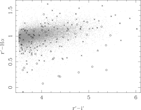
Figure 1: IPHAS colour-colour diagram of the “extremely red” region showing the positions of all the extremely red stellar objects (ERSOs) as dots and the sources observed as symbols: cross symbols are O-rich sources, circles are S-type stars, triangles are carbon stars and asterisks are spectrally unidentified sources.

2.1 Observational procedure and data reduction

Each object was observed using both the lrzj8 (0.89-1.51 $\mu$m) and lrhk (1.40-2.39 $\mu$m) grisms, giving continuous coverage from 0.89-2.39 $\mu$m through the z, J, H and K bands. The resolving power was 700 for both grisms, allowing many molecular features and the strongest metal lines to be identified. The spatial scale was 0.25^′′ pixel^-1, and the slit width used during the observations was 1^′′, aligned along the parallactic angle. Observations were performed using an “ABBA” telescope-nodding pattern, placing the source in two positions along the slit, A and B, separated by 80^′′. Exposure times for each grism are listed in Table LABEL:observation_list. The bias and dark levels of most near-IR detectors are unstable with time, therefore LIRIS takes a “pre-read” image, which is automatically subtracted from the “post-read” exposure (also known as “double-correlated sampling”).

Table 1: Sources observed with LIRIS on the WHT. Mean photometric magnitudes are taken from all IPHAS measurements. Spectral types for all sources are also listed (only the temperature class is listed since all sources are believed to be giants). For S-type stars, spectral types are listed as SX/Y, where X is the temperature index (not available for all sources) and Y is the abundance index. Carbon stars are listed as “C”, as further classification was not possible. Unclassified O-rich stars are listed as “K0-M2” and completely unclassified stars are listed as “U”. Stars with emission lines are denoted with “e”. Previous identifications are listed if available from the Simbad astronomical database. Other notes: Variable stars are identified based on the presence of strong water vapour bands. Oxygen rich sources with high C/O ratios (C/O $\sim$ 0.9-0.95) are identified based on very strong H-band CO lines and no OH lines. Carbon stars with the suspected C₂H₂ feature in their H-band spectra are also noted.

No.	Name	Photometry			Exposures (s)		Spectral	Notes
		r’	i’	H$\alpha$	zJ	HK	type
ERSO1	IPHAS J184857.78-021536.6	21.721	16.039	20.805	4.0	5.0	M6
ERSO2	IPHAS J183432.01-011828.1	21.972	16.311	20.723	4.0	10.0	M7.5
ERSO3	IPHAS J184859.24-011234.1	21.838	15.817	20.698	3.0	8.0	M6	C/O $\sim$ 0.9-0.95
ERSO4	IPHAS J190745.00+032227.4	19.366	15.096	16.747	10.0	30.0	M4
ERSO5	IPHAS J190843.09+032752.3	20.200	15.959	17.802	20.0	20.0	M3
ERSO6	IPHAS J190906.83+033654.5	20.503	15.870	17.981	15.0	20.0	M4
ERSO7	IPHAS J191402.54+024348.1	18.055	14.107	17.529	3.0	5.0	M9.5	Variable
ERSO8	IPHAS J191014.09+112409.1	16.667	12.671	16.043	3.0	8.0	M6
ERSO9	IPHAS J191033.49+113644.6	17.325	13.295	16.476	8.0	14.0	M6
ERSO10	IPHAS J190836.69+113729.3	17.370	13.684	16.912	4.0	10.0	M6
ERSO11	IPHAS J191016.76+114134.4	17.202	13.304	16.737	8.0	10.0	SX/6
ERSO12	IPHAS J190926.40+114140.0	18.015	14.107	17.293	6.0	20.0	M7
ERSO13	IPHAS J194626.37+270936.0	17.081	13.541	16.121	7.0	20.0	M5
ERSO14	IPHAS J185412.60-040704.6	17.419	13.724	16.314	10.0	15.0	M6
ERSO15	IPHAS J193123.25+184244.7	15.648	11.972	14.585	4.0	8.0	M6
ERSO16	IPHAS J000701.80+654917.9	16.953	12.850	15.937	4.0	10.0	SX/5
ERSO17	IPHAS J002455.87+654955.7	16.815	13.000	15.836	3.0	8.0	M2
ERSO18	IPHAS J004918.50+652822.9	17.141	13.422	16.115	10.0	20.0	M3
ERSO19	IPHAS J001841.82+660645.4	17.366	13.101	16.192	5.0	15.0	M8.5	C/O $\sim$ 0.9-0.95
ERSO20	IPHAS J002531.86+621912.6	17.289	13.646	16.187	8.0	12.0	M6.5
ERSO21	IPHAS J005934.24+651815.1	17.977	14.027	16.961	10.0	50.0	M8.5	Variable
ERSO22	IPHAS J010743.47+630523.0	17.071	13.471	16.731	3.0	6.0	SX/6
ERSO23	IPHAS J021849.42+622138.8	17.996	14.369	17.612	20.0	15.0	SX/6
ERSO24	IPHAS J023951.19+555352.3	17.470	13.210	16.897	3.0	3.0	SX/6
ERSO25	IPHAS J025402.88+575126.7	18.920	13.740	17.758	2.9	3.0	U	Noisy spectrum
ERSO26	IPHAS J030552.92+542054.2	20.045	14.924	18.719	5.0	20.0	M10.5	Variable
ERSO27	IPHAS J010744.59+590302.0	20.140	14.681	19.125	3.0	8.0	SX/6e
ERSO28	IPHAS J033511.00+505830.2	14.799	11.034	14.076	3.0	4.0	SX/6
ERSO29	IPHAS J033938.45+521452.8	15.477	11.906	14.351	3.0	6.0	M6.5
ERSO30	IPHAS J034517.16+561951.5	15.874	11.867	14.760	3.0	3.0	S2/4
ERSO31	IPHAS J025540.05+602012.0	15.907	11.861	14.483	3.0	6.0	S3/4
ERSO32	IPHAS J230150.16+613946.2	20.214	14.848	19.392	3.0	3.0	SX/6
ERSO33	IPHAS J184927.44+034408.8	20.254	14.983	19.070	5.0	10.0	SX/4
ERSO34	IPHAS J190141.34+063409.8	21.428	16.609	20.283	20.0	30.0	M5
ERSO35	IPHAS J184747.70+005111.2	21.943	17.065	21.051	6.0	20.0	M7.5
ERSO36	IPHAS J190032.96+030112.7	21.899	16.334	20.489	15.0	10.0	M5.5
ERSO37	IPHAS J192009.24+102007.1	19.347	15.013	18.205	6.0	15.0	M6
ERSO38	IPHAS J185316.59-023712.6	21.124	16.300	19.986	10.0	20.0	M7
ERSO39	IPHAS J190245.00+075338.5	20.076	15.059	18.935	3.0	15.0	M7.5
ERSO40	IPHAS J203602.11+380401.6	19.806	15.093	18.759	3.0	10.0	SX/5
ERSO41	IPHAS J183704.11-010704.2	20.947	16.227	19.962	15.0	30.0	M5
ERSO42	IPHAS J190823.19+054151.7	20.371	16.055	19.484	10.0	30.0	M5
ERSO43	IPHAS J184925.41+042234.7	17.080	12.439	15.859	3.0	3.0	M9.5	Variable
ERSO44	IPHAS J192426.56+235545.8	19.446	15.744	17.608	6.0	12.0	M9	Variable
ERSO45	IPHAS J190943.96+134240.5	18.838	14.812	17.658	12.0	30.0	M6.5
ERSO46	IPHAS J215203.82+574915.5	18.341	14.268	17.145	3.0	6.0	M6.5
ERSO47	IPHAS J184336.32+010256.3	19.514	15.189	18.129	15.0	20.0	K0-M2
ERSO48	IPHAS J214953.49+540713.9	18.512	14.441	17.256	8.0	12.0	M5.5
ERSO49	IPHAS J202810.38+375759.8	18.814	15.170	17.561	8.0	15.0	M3
ERSO50	IPHAS J190848.37+033659.1	19.074	14.946	17.450	15.0	30.0	M6
ERSO51	IPHAS J214234.08+572008.9	16.769	12.543	15.270	3.0	3.0	K0-M2
ERSO52	IPHAS J202503.70+371340.6	18.456	13.488	17.183	3.0	3.0	S6/2
ERSO53	IPHAS J204417.37+414718.0	18.688	14.726	17.876	3.0	6.0	K0-M2
ERSO54	IPHAS J200921.71+282602.7	19.075	14.625	18.524	3.0	10.0	M9	C/O $\sim$ 0.9-0.95
ERSO55	IPHAS J200959.88+280809.3	18.990	14.563	18.193	3.0	6.0	M7
ERSO56	IPHAS J203609.30+402950.9	19.623	14.548	19.219	3.0	3.0	SX/7
ERSO57	IPHAS J201448.15+361245.1	19.917	15.379	19.340	6.0	15.0	K0-M2
ERSO58	IPHAS J230620.82+600432.9	19.028	13.946	17.877	3.0	4.0	M8.5e
ERSO59	IPHAS J211755.60+473811.1	19.237	14.023	17.941	3.0	8.0	M10.5	Variable
ERSO60	IPHAS J195445.65+325937.9	20.583	17.011	19.814	6.0	40.0	C	C2H2
ERSO61	IPHAS J231655.24+602600.6	17.109	12.382	15.677	3.0	6.0	M8.5	Variable
ERSO62	IPHAS J005317.94+623611.5	20.680	15.204	19.295	4.0	15.0	M6.5
ERSO63	IPHAS J020611.54+610528.1	19.627	14.668	18.603	4.0	12.0	S4/4
ERSO64	IPHAS J230925.46+615258.6	21.119	16.220	19.831	6.0	15.0	M5
ERSO65	IPHAS J011803.17+635545.3	19.658	15.178	18.448	4.0	12.0	M8.5	Variable
ERSO66	IPHAS J011847.64+665247.8	18.083	13.528	16.821	6.0	15.0	M5
ERSO67	IPHAS J204519.10+404011.4	17.342	12.815	15.436	3.0	8.0	M6
ERSO68	IPHAS J202243.51+415428.2	21.612	16.500	19.732	10.0	20.0	M5.5
ERSO69	IPHAS J192423.87+142621.5	19.897	15.793	18.540	30.0	45.0	M5
ERSO70	IPHAS J203908.44+392129.5	22.680	17.726	20.723	30.0	60.0	M4
ERSO71	IPHAS J190810.54+110315.8	19.830	15.443	18.388	30.0	45.0	M4
ERSO72	IPHAS J191007.21+112222.0	18.918	14.123	17.375	5.0	40.0	M7
ERSO73	IPHAS J202922.55+400537.2	19.790	16.185	19.876	12.0	25.0	M2
ERSO74	IPHAS J210511.40+440531.2	17.208	13.529	16.693	25.0	45.0	K0-M2
ERSO75	IPHAS J193344.25+194748.3	20.348	16.551	20.006	36.0	45.0	K0-M2
ERSO76	IPHAS J211036.95+495249.2	18.912	14.887	18.835	8.0	40.0	SX/7e
ERSO77	IPHAS J200510.62+344753.9	20.691	16.255	20.125	20.0	45.0	K0-M2
ERSO78	IPHAS J192619.66+170909.7	21.643	18.031	20.979	60.0	60.0	K0-M2
ERSO79	IPHAS J192601.33+140638.6	21.530	16.683	20.909	8.0	25.0	K0-M2
ERSO80	IPHAS J190708.46+044931.6	18.617	13.831	18.323	40.0	60.0	SC9/8e
ERSO81	IPHAS J192706.10+181527.7	21.212	17.517	20.917	40.0	60.0	K0-M2
ERSO82	IPHAS J192611.47+140919.4	21.167	17.111	20.651	25.0	60.0	K0-M2
ERSO83	IPHAS J190752.06+075040.4	20.447	16.704	19.761	30.0	60.0	M4.5
ERSO84	IPHAS J035507.56+493357.6	19.512	14.760	18.285	3.0	6.0	S5/3
ERSO85	IPHAS J041023.81+510725.2	17.480	13.694	16.592	5.0	25.0	M3
ERSO86	IPHAS J041503.75+501122.9	15.638	11.831	14.676	3.0	8.0	SX/5
ERSO87	IPHAS J042606.70+482016.7	15.800	12.274	14.777	3.0	10.0	K0-M2
ERSO88	IPHAS J043215.53+423614.6	16.804	12.575	15.495	3.0	6.0	M10e	Variable
ERSO89	IPHAS J053653.80+311306.0	17.263	13.435	16.234	7.0	30.0	K0-M2
ERSO90	IPHAS J054141.41+295318.2	15.779	11.697	14.697	3.0	6.0	SX/5
ERSO91	IPHAS J054434.74+281759.5	15.796	11.795	14.604	3.0	3.0	M9.5	Variable
ERSO92	IPHAS J054529.94+290705.2	16.869	12.034	15.689	3.0	3.0	M10.5	Variable
ERSO93	IPHAS J054837.39+243947.0	16.209	12.659	15.180	6.0	15.0	K0-M2
ERSO94	IPHAS J054921.16+264624.3	19.270	15.736	18.565	15.0	30.0	K0-M2
ERSO95	IPHAS J063206.40+041718.2	20.305	16.113	19.430	30.0	60.0	K0-M2
ERSO96	IPHAS J063455.83+043847.1	16.147	12.003	14.906	6.0	15.0	M8.5	Variable
ERSO97	IPHAS J063552.51-030815.8	17.287	13.307	16.048	5.0	15.0	M8	Variable
ERSO98	IPHAS J184029.02+035812.6	17.247	13.602	16.129	15.0	15.0	M6.5	C/O $\sim$ 0.9-0.95
ERSO99	IPHAS J185904.00+081851.1	19.728	15.178	18.575	20.0	30.0	M6
ERSO100	IPHAS J190010.63+073538.7	19.472	15.378	18.669	15.0	20.0	K0-M2e
ERSO101	IPHAS J185136.91+020514.0	19.206	14.751	18.231	20.0	30.0	M5
ERSO102	IPHAS J185131.52+020517.9	19.600	16.018	18.769	30.0	30.0	K0-M2
ERSO103	IPHAS J192718.83+202656.9	18.572	14.828	17.547	40.0	60.0	K0-M2
ERSO104	IPHAS J200348.11+290553.2	16.341	12.474	15.688	10.0	20.0	SX/5
ERSO105	IPHAS J203806.06+405336.6	19.689	15.306	18.887	5.0	20.0	U	C/O $\sim$ 0.9-0.95
ERSO106	IPHAS J203914.32+413046.4	20.184	16.329	19.417	30.0	60.0	M5.5
ERSO107	IPHAS J204834.99+442726.8	19.590	15.939	18.883	25.0	60.0	K0-M2
ERSO108	IPHAS J203421.64+412227.8	18.833	15.307	17.934	15.0	30.0	K0-M2
ERSO109	IPHAS J192703.20+203707.8	17.086	13.250	15.988	20.0	20.0	M2
ERSO110	IPHAS J185800.71+072719.4	18.867	15.135	17.969	60.0	60.0	M5
ERSO111	IPHAS J203440.02+415433.0	18.452	14.670	17.600	20.0	30.0	K0-M2
ERSO112	IPHAS J203511.15+403556.9	20.085	16.013	19.175	30.0	60.0	K0-M2
ERSO113	IPHAS J211510.01+520218.0	20.735	16.946	20.096	20.0	100.0	C
ERSO114	IPHAS J184315.46+035308.8	18.545	13.805	17.217	5.0	30.0	M7.5e
ERSO115	IPHAS J185923.26+081024.7	18.414	13.854	17.286	4.0	20.0	M6.5
ERSO116	IPHAS J185849.22+074453.2	18.257	14.481	17.266	30.0	30.0	U	Noisy spectrum
ERSO117	IPHAS J185115.41+013909.8	21.098	16.903	20.396	12.0	60.0	C	C2H2
ERSO118	IPHAS J184041.73-012350.8	20.621	16.778	19.608	60.0	100.0	K0-M2
ERSO119	IPHAS J204058.42+403347.7	21.204	16.968	20.654	3.0	30.0	C	C2H2
ERSO120	IPHAS J185216.79-032928.9	19.599	15.988	18.671	60.0	100.0	K0-M2
ERSO121	IPHAS J212057.68+470041.4	20.293	15.932	20.071	5.0	20.0	SX/6
ERSO122	IPHAS J184134.15-022446.0	21.844	16.557	20.254	60.0	100.0	M6.5
ERSO123	IPHAS J194854.17+295316.1	17.168	13.561	16.031	15.0	30.0	M6
ERSO124	IPHAS J202632.12+410018.8	18.837	15.148	18.055	6.0	60.0	K0-M2
ERSO125	IPHAS J203219.30+404603.6	20.159	16.368	19.489	15.0	100.0	K0-M2
ERSO126	IPHAS J203423.56+402354.8	19.999	16.411	19.267	15.0	60.0	K0-M2
ERSO127	IPHAS J203538.75+413102.0	19.728	16.154	19.070	20.0	60.0	K0-M2
ERSO128	IPHAS J203653.35+411501.2	18.990	15.425	18.151	20.0	60.0	K0-M2
ERSO129	IPHAS J203232.98+404701.8	20.066	15.502	19.142	5.0	30.0	M5.5
ERSO130	IPHAS J204207.60+413051.3	20.203	16.057	19.091	40.0	40.0	M4
ERSO131	IPHAS J202905.52+394245.8	20.496	14.624	19.151	3.0	5.0	M6.5
ERSO132	IPHAS J203250.04+414720.8	21.806	16.431	21.466	10.0	30.0	SX/7
ERSO133	IPHAS J204114.29+405617.0	20.357	16.597	19.581	20.0	60.0	U
ERSO134	IPHAS J203053.66+403232.6	20.483	16.576	19.690	12.0	30.0	M5
ERSO135	IPHAS J184226.36-021737.5	20.343	15.807	19.244	40.0	100.0	M6
ERSO136	IPHAS J192459.62+170653.4	20.337	15.146	19.619	3.0	10.0	C
ERSO137	IPHAS J202012.43+384657.2	19.816	15.426	19.605	5.0	20.0	SX/6
ERSO138	IPHAS J203741.24+412137.0	20.228	15.905	19.288	20.0	30.0	M4
ERSO139	IPHAS J205032.35+413459.9	18.175	14.647	17.200	20.0	40.0	K0-M2

Table 1: continued

No.	Name	Previous identifications
ERSO23	IPHAS J021849.42+622138.8	Variable star (Usatov & Nosulchik, 2008)
ERSO24	IPHAS J023951.19+555352.3	EI Per (M8, Mira) (Bidelman, 1987)
ERSO26	IPHAS J030552.92+542054.2	V673 Per (Mira) (Kazarovets et al., 2003)
ERSO27	IPHAS J010744.59+590302.0	V890 Cas (Mira) (Kazarovets et al., 2003)
ERSO43	IPHAS J184925.41+042234.7	Haro Chavira 35 (M7) (Skiff, 1999)
ERSO51	IPHAS J214234.08+572008.9	Variable star (Kun, 1987)
ERSO58	IPHAS J230620.82+600432.9	QU Cep (M6, Mira) (Rosino et al., 1976)
ERSO60	IPHAS J195445.65+325937.9	WC Wolf-Rayet? (Cohen, 1995)
ERSO61	IPHAS J231655.24+602600.6	V563 Cas (M6e) (Rosino et al., 1976)
ERSO62	IPHAS J005317.94+623611.5	M4 (Ichikawa, 1981)
ERSO80	IPHAS J190708.46+044931.6	CSS2 30 (S-type) (Stephenson, 1990)
ERSO91	IPHAS J054434.74+281759.5	IZ Tau (M9, Mira) (Stephenson, 1992)
ERSO92	IPHAS J054529.94+290705.2	V530 Aur (M8, OH/IR) (Iyengar & MacConnell, 1998)
ERSO117	IPHAS J185115.41+013909.8	Carbon star (Kwok et al., 1997)
ERSO119	IPHAS J204058.42+403347.7	Carbon star (Kwok et al., 1997)
ERSO136	IPHAS J192459.62+170653.4	OH/IR (Le Squeren et al., 1992), Carbon star (Kwok et al., 1997)

Table 2: Observed sources with previous identifications in the literature. See Section 4.3 for notes on individual sources of interest.

The data were reduced following standard procedures for near-IR spectroscopy, using IRAF and the LIRIS Data Reduction dedicated software. Flat fields were taken at the beginning of each night with each grism and filter setup and applied to all observations as appropriate. Bad pixels were also removed at this stage of data analysis using a bad pixel mask produced from a series of short and long exposures taken at the beginning of each night.

Consecutive pairs of AB two-dimensional spectra were subtracted to remove the sky background and then co-added. Spectra were then extracted from the resulting frames and wavelength-calibrated before co-adding all the frames to provide the final spectrum. The wavelength calibration was provided by observations of argon and xenon lamps. Observations of near-IR standard stars (see Table 3) were made throughout each night. The choice of a slit much narrower than the seeing does not allow us to perform flux calibration using our standard star observations, and due to the intrinsic variability of the majority of these sources, would be of limited use.

Name	Spectral type	RA	Dec	Magnitudes					Nights
		(J2000)	(J2000)	B	V	J	H	Ks	observed
HIP71819	G2V	14 41 28.77	+13 36 05.3	8.99	8.40	7.178	6.933	6.873	1, 2, 3, 4, 5
HIP92865	O8V	18 55 23.13	+09 20 48.1	9.10	8.64	7.452	7.377	7.328	1, 4, 5
HIP96037	G2V	19 31 37.81	+17 46 58.6	8.90	8.26	6.954	6.588	6.542	2, 3

Table 3: Infrared standard stars observed each night with LIRIS on the WHT and used for data reduction. Photometric magnitudes were obtained from the Simbad astronomical database.

Near-IR spectroscopic observations are affected by telluric absorption due to scattering and absorption by atmospheric molecules, particularly H₂O and CO₂. Telluric correction was performed by dividing science spectra by the ratio of a G2V standard star (see Table 3) and a rebinned solar model spectrum from Kurucz (1979), scaled to the airmass of the observation. For those telluric features that do not only vary with airmass (such as H₂O) we varied the strength of this correction until an appropriate continuum could be restored. We found this method was particularly effective in correcting telluric absorption in regions with small absorption features where the underlying spectrum contained valuable information. Finally, each spectrum was divided by an estimated continuum to normalise them.

2.2 The final data

The resulting data set consists of 139 spectra with a resolution of 20 Å in the $J$ band and and 33 Å in the $H$ and $K$ bands. Using multiple observations of the O8V standard star HIP92865 (Table 3), we estimate a typical signal-to-noise ratio of 30. This value drops considerably in regions of strong telluric absorption. The reduced spectra are presented in a series of figures throughout this paper and will also be available in tabulated form through the VizieR service. A number of spectra were presented by Wright et al. (2008), but we present the full sample here, continuing the numbering system used by those authors.

3 Spectral analysis and classification

In this section, we first describe the character of the LIRIS spectra we have obtained, ordering the presentation by atmospheric window ($J$ first, followed by $H$ and then $K$). When appropriate we further break down the discussion according to the three main groupings of AGB stars by photospheric pattern (O-rich stars, S-type stars and carbon stars). With this overview in place, we move on to the task of formal classification (Section 3.4).

It has been commented before (Wallace et al., 2000) that the $J$ window is often the most useful in estimating spectral type, containing features due to TiO and VO in O-rich stars, ZrO in S-type stars and C₂ and CN in carbon stars. The $H$ band includes two dominant sequences due to the OH and CO molecules, the former only being found in O-rich stars, as well as a strong C₂ feature indicative of carbon stars. The wings of the $H$ window are also particularly influenced by water vapour bands typical of the outer atmospheres of highly variable O-rich stars. The $K$ window is less distinctive, being dominated by the CO first overtone bands present in the spectra of all cool evolved stars.

Classification of the LIRIS spectra is based on a range of spectral libraries (e.g. Joyce, 1998; Kleinmann & Hall, 1986; Lançon & Wood, 2000; Wallace et al., 2000) and on discussions of the variation of near-IR molecular signatures with effective temperature and chemical abundances (e.g. Brett, 1990; Hinkle et al., 1989; Keenan & Boeshaar, 1980; Origlia et al., 1993). Where we need to extend these schemes, we will draw attention to it. Derived spectral types are listed in Table LABEL:observation_list.

We will also draw attention to certain objects and spectral features of special interest, including those that do not fit easily within the classification scheme. We note that at the resolution of our spectra, only the strongest atomic lines are visible in all objects observed. Given that the existing classification schemes do not make use of atomic lines, we will not discuss these in detail here.

3.1 The spectra in the $J$ window

3.1.1 M-type (O-rich) stars in the J-band

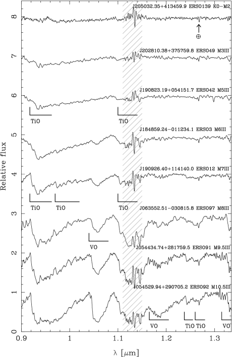
Figure 2: J-band spectra of oxygen-rich evolved stars (see Table LABEL:observation_list for details) shown in order of decreasing effective temperature. Each spectrum has been corrected for telluric absorption and has been divided by an adopted continuum. The spectra have been separated by integer values of normalised flux to make each clear and visible. The shaded area indicates a region of low atmospheric transmission where telluric correction was unable to recover a useful spectrum. Prominent molecular features have been marked, in addition to an O₂ telluric feature at 1.27 $\mu$m.

Figure 2 shows J-band spectra for a series of O-rich giant stars. The spectra contain molecular bands primarily due to TiO and, in later spectral types, VO, which identify them as O-rich stars (c.f. Phillips, 1969; Brett, 1990). The TiO bands appear around $\sim$3600 K ($\sim$M3) for giant stars (Lançon et al., 2007) and get deeper as the temperature decreases. The most prominent of these is the TiO $\epsilon$ $\Delta v=-1$ feature at 0.92 $\mu$m (Schiavon & Barbuy, 1999). This is coincident with a telluric absorption feature that we were able to successfully correct for in the majority of spectra due to its relative shallowness. For sources that are faint in this region, reconstructing the continuum via telluric correction often produced high noise levels and this feature was not always clear.

The smaller neighbouring feature at 0.97 $\mu$m is due to the TiO $\delta$ $\Delta v=-1$ transition (Brett, 1990) and we find this discernible from M5-M6 onwards though it is often lost in its deeper neighbour. Other TiO lines in the J-band include the $\phi$ $\Delta v=0$ system at 1.1 $\mu$m (just visible on the edge of a telluric H₂O feature) and the $\phi$ $\Delta v=-1$ system at 1.25 $\mu$m, whose two bandheads become visible from M7 onwards.

In late M-type stars the VO molecule becomes the most dominant feature, typically appearing for T${}_{eff}\leq 3200$ (later than M6, Joyce et al., 1998) and growing with decreasing temperature. The largest of these is the 0-0 head of the $A^{4}\Pi-X^{4}\Sigma^{-}$ $\Delta v=0$ transition at 1.046 $\mu$m (Hinkle et al., 1989). Smaller VO features at 1.168-1.181 $\mu$m due to the $\Delta v=-1$ transition of the A-X system are also visible for very late type stars (Brett, 1990). The $\Delta v=-2$ feature is often visible at 1.325 $\mu$m, but can get lost in the deep telluric feature longwards of it (Hinkle et al., 1989).

Other features present in our spectra are a large number of atomic lines from neutral species, the strongest of which include Mn i 1.295 $\mu$m and Al i 1.313 $\mu$m. We also see the hydrogen emission lines P$\gamma$ 1.093 $\mu$m and P$\beta$ 1.281 $\mu$m in some of our spectra. The 3rd overtone lines of CO should lie around 1.16-1.24 $\mu$m, but Hinkle et al. (1989) searched for them in higher resolution J-band spectra and were unable to find them. We therefore rule out any of the features in this region as being due to CO and believe that the abundant neutral atomic lines predicted in this region of the spectrum by Wallace et al. (2000) offer a more likely explanation.

3.1.2 MS and S-type stars in the J-band

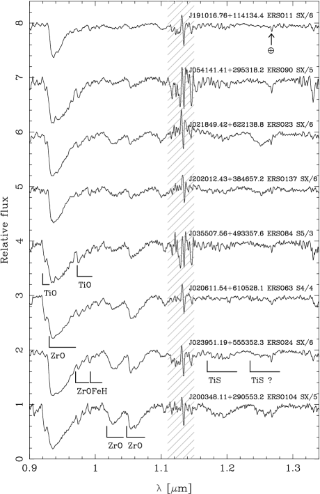
Figure 3: J-band spectra of S-type evolved stars, as per Figure 2 and shown in approximate order of increasing strength of the 1.0-1.1 $\mu$m ZrO features.

S-type giant stars are believed to be intermediate between O-rich stars (C/O $<$ 1) and C-rich stars (C/O $>$ 1) as part of an evolutionary sequence M-MS-S-SC-C (where the intermediate types show dual chemistries). This sequence is believed to be caused by an increase in the C/O ratio due to dredged-up carbon, but the abundance of Zr (Vanture & Wallerstein, 2002) and variations in the photospheric temperature throughout pulsation cycles can also influence the observed spectral type (e.g. Zijlstra et al., 2004). The photospheres of S-type stars exhibit near unity C/O ratios and enrichment of the s-process elements Zr, Y, La and Ce (Smith & Lambert, 1990). With carbon and oxygen almost completely locked up in CO, the sulphides of these heavy elements attain an abundance equal to the oxides (Joyce et al., 1998).

Figure 3 shows J-band spectra for a group of S-type stars which primarily feature bands due to ZrO. The strongest ZrO band visible in our spectra is at 0.93-0.96 $\mu$m (the $b^{\prime 3}\Pi-a^{3}\Delta$ system 0-0 bandhead, Phillips et al., 1979). Its position is almost coincident with the 0.92 $\mu$m TiO feature, but the contributions from the two features may be separated and estimated. Some sources (e.g. ERSO 24) show no evidence for the TiO feature, while others (e.g. ERSO 63) show the TiO bandhead at 0.92 $\mu$m in addition to a deeper ZrO bandhead at 0.93 $\mu$m and are likely the MS-type transition objects. The form of the ZrO feature is clearly distinguishable from those due to TiO (see Figures 2 and 3).

The most unmistakable ZrO bands are the pair at 1.03 and 1.06 $\mu$m (the $a^{3}\Delta$ 0-1 and $B^{1}\Pi-A^{1}\Delta$ 0-0 band heads respectively, Hinkle et al., 1989), which are easily identifiable in contrast to the VO feature found in O-rich sources. Many of these sources also show the 0.974 $\mu$m ZrO feature (the head of the B-A $\Delta\nu=-1$ band, Davis & Hammer, 1981) and the 0.99 $\mu$m FeH band (the ${}^{4}\Delta-^{4}\Delta$ 0-0 head, Lambert & Clegg, 1980), both visible in the long-wavelength wing of the strong 0.93 $\mu$m ZrO feature. All these features have strengths dependent on the photospheric temperature, C/O ratio and heavy element abundances.

Visible in a large number of our S-type star spectra is a feature at 1.25 $\mu$m which Joyce et al. (1998) observed in their spectra of S-types, but were unable to conclusively associate with a specific molecule. It coincides with the positions of the ZrS b^′-a $\Delta\nu=0$ sequence and the TiS A-X $\Delta\nu=0$ sequence (Jonsson et al., 1992), both of which may contribute to the feature. Of the sources that display this feature we note two types. The first type shows the TiS A-X $\Delta\nu=-1$ sequence at 1.17-1.22 $\mu$m at a similar strength to the 1.25 $\mu$m feature (e.g. ERSO 24, ERSO 104, or R And, Jonsson et al., 1992), while the second type shows either a much weaker or completely absent 1.17-1.22 $\mu$m feature (e.g. ERSO 23 or R Cyg, Joyce et al., 1998). We suggest that in the first set of cases the 1.25 $\mu$m feature originates from the TiS molecule, while in the second set of cases the feature is either purely ZrS or a combination of TiS and ZrS. This is supported by the position of the 1.25 $\mu$m feature in ERSO 23 appearing at a slightly shorter wavelength to that in ERSOs 24 or 104.

3.1.3 Carbon stars in the J-band

Figure 4: J-band spectra of carbon stars as per Figure 2 and shown in order of increasing CN feature strength.

Figure 4 shows J-band spectra for four carbon stars in order of increasing feature strength. The spectra of carbon stars in the J-band primarily show features due to the molecules CN and C₂. Clearly visible in our spectra are the CN 1-0 and 0-0 bandheads at 0.914 and 1.088 $\mu$m (both part of the Red A²$\Sigma$-X²$\Sigma$⁺ system, Joyce et al., 1998).

Also visible in the spectra of some objects are bandheads due to the Phillips and Ballick-Ramsay systems of the C₂ molecule (Hunaerts, 1967; Querci et al., 1974). The most prominent of these are the Phillips 1-0 transition at 1.02 $\mu$m, the Ballick Ramsay 2-0 transition at 1.174 $\mu$m and the Phillips 0-0 transition at 1.207 $\mu$m.

Carbon star spectra often show a highly ”grassy” appearance which has been attributed to minor CN features and contributions from additional C-rich absorbers across these bands (Joyce et al., 1998). A high fraction of the isotope ¹³C can also lead to many weak molecular features alongside those due to ¹²C.

3.2 The spectra in the $H$ window

Unlike the J-band, the spectral differences between M, S and C-type evolved stars in the H-band are much more subtle. The band is bordered on both sides by deep telluric H₂O features where transmission regularly drops to zero in our spectra. The molecular features in the H-band are principally due to the CO 2nd overtone series and the OH molecule.

3.2.1 CO and OH bands

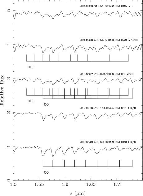
Figure 5: H-band spectra of five evolved stars shown top to bottom in approximate order of C/O ratio increasing towards unity. The spectra have been divided by an adopted continuum and are separated by integer values of normalised flux. The CO and OH series are shown.

The CO 2nd overtone ($\Delta v=-3$) series extends from 1.56 $\mu$m (3-0) to longer wavelengths with higher transition features and develops at temperatures below $\sim 5000$ K (Lançon et al., 2007). The strongest transition is expected to be (6-3) at 1.62 $\mu$m, with strengths decreasing before and afterwards (Origlia et al., 1993), though at our resolution this is hard to verify. Bands from the molecular isotope ¹³CO are also present in a number of our H-band spectra, though the majority of their lines are confused with lines from ¹²CO or OH. Lines of ¹³CO in the H-band are very weak even for high ¹³C/¹²C ratios because of the low optical depths of the ¹²CO second overtone bands (lines from the first overtone of ¹³CO in the K-band are easier to detect).

Some of the CO bands are blended with lines from OH, a molecule that is responsible for many features across the H-band, with the strongest at 1.537, 1.625 and 1.690 $\mu$m. As the C/O ratio increases, the strength of the OH bands gradually decreases (see sequence in Figure 5), while the strength of the CO bands increases. M-type stars typically show a mixture of equal strength CO and OH lines, while for S-type stars the OH lines are very weak. At C/O $\sim$ 1 the CO bands reach their peak and become well defined. For carbon stars (where C/O $>$ 1), the CO lines wane in strength since less oxygen is available (see Section 3.2.3). Many of the weak unidentified features in the H-band are thought to be due to CN, which produces many small features, giving the impression of a noisy looking continuum (Origlia et al., 1993).

3.2.2 Water vapour bands

The cool extended atmospheres of highly variable evolved stars enable the formation of H₂O, which can cause deep features coincident with the telluric absorption bands, but significantly broader (e.g. Matsuura et al., 1999). Their presence implies a source with a large amplitude of variability ($\delta V>1.7$, Lançon & Wood, 2000). The exact shape of the water bands is highly dependent on the exact conditions in the outer atmosphere and varies considerably throughout the pulsation period. The observation of strong H₂O bands is evidence of a highly variable very late-type star, though absence of them does not disprove this. Figure 6 shows examples of the effects of water vapour bands on H-band spectra.

Figure 6: Spectra of five stars in the H-band showing the strong effects of certain molecular features. No telluric correction has been applied to these sources and the effects of telluric absorption are visible at the short and long wavelength ends of the spectra in the ranges 1.4-1.5 $\mu$m and 1.75-1.85 $\mu$m (ERSO 12 is an example of the typical levels of telluric absorption before correction has been applied). ERSOs 12, 21, and 26 show the increasing influence of photospheric water vapour bands from negligible to very strong for very late-type O-rich sources (the absorption in the wings of ERSO 12 is believed to be due entirely to telluric water vapour and is typical of uncorrected H-band spectra). ERSOs 113 and 117 show the effects of C-rich molecular features on the $H$-band. CN absorption is responsible for the slope of the spectra from 1.5 $\mu$m longwards (without CN absorption the short-wavelength absorption from telluric H₂O would be similar to that of ERSO 12 and the full CO sequence would be visible). ERSO 117 also shows the unidentified feature at 1.53 $\mu$m which has been suggested to be due to C₂H₂.

We find evidence for water vapour in 13 of our sources, including four with very strong absorption bands (all of which are of type M9.5 or later). The fraction of sources in our sample showing these absorption bands increases towards later spectral types, going from 57% at M8 (4 of 7 stars) to 60% at M9 (3 of 5 stars) and 100% at M10 (4 stars).

3.2.3 Carbon stars in the H-band

At C/O ratios above unity the H-band CO lines decrease in strength and the CN 0-1 bands become dominant. Because the head of this series lies in the telluric absorption feature around 1.4 $\mu$m, the band head is lost in a region of near-zero transmission. However, the series extends across most of the H-band and causes a gradient in the continuum across the band (see Figure 6). Often the most notable feature in the near-infrared spectra of carbon stars is the C₂ band at 1.77 $\mu$m (the Ballick-Ramsay A${}^{\prime 2}\Sigma_{g}^{-}$-X${}^{\prime 3}\Pi_{u}$ (0-0) band, Hunaerts, 1967), which is usually the strongest of all the C₂ bands in the near-infrared (Loidl et al., 2001).

Three of our five carbon stars also show an unidentified feature at 1.53 $\mu$m (see Figure 6) that has previously been observed in cool and high Galactic latitude carbon stars (e.g. Joyce, 1998). The feature is thought to be due to the second overtone C-H stretch from molecules such as HCN or C₂H₂ and its presence is well correlated with a feature at 2.45 $\mu$m observed in laboratory spectra of C₂H₂ (Goebel et al., 1981). However Joyce (1998) found that the 1.53 $\mu$m feature was not well correlated with a 3.1 $\mu$m feature also associated with the molecules HCN and C₂H₂. We calculated spectra of C₂H₂ using the HITRAN line lists (Rothman et al., 2009) that includes lines from C₂H₂ (Hachtouki & Auwera, 2002). The 1.53 $\mu$m feature in our spectra matches well with the R- and P-branches of C₂H₂, confirming it as a likely carrier. The C₂H₂ cross section at 1.53 $\mu$m is a factor $\sim$7 larger than that of HCN, such that HCN would require a column density $\sim$7 times that of C₂H₂ to produce the same absorption. It is therefore easier to explain the observed feature with C₂H₂ unless HCN is very abundant. The opposite is true for the 3.1 $\mu$m feature (Aoki et al., 1998), which could explain the lack of correlation between the strength of this and the 1.53 $\mu$m feature observed by Joyce (1998) if they had different dominant contributors.

3.3 The spectra in the $K$ window

Figure 7: K-band spectra of six evolved stars with different chemical types and temperature classes. Each spectrum has been divided by an adopted continuum and separated by integer values of normalised flux.

As in the H-band the K-band is dominated by absorption from CO, though the features are stronger here. The edges of the K-band are defined by strong telluric H₂O features and two strong CO₂ features around 2 $\mu$m. The slope of the spectra in the K-band is also affected by H₂O absorption at the long wavelength end of the band, with many minor features contributing to the overall shape of the spectrum (Kleinmann & Hall, 1986).

Spectra of six evolved stars in the $K$ band of different spectra types are shown in Figure 7. Our spectra feature four lines from the first overtone ($\Delta v=-2$) series of ¹²CO, starting at the 2.29 $\mu$m bandhead (2-0), with higher order terms extending to longer wavelengths. In M-type stars the strength of these lines increases with increasing luminosity and decreasing temperature and some attempts have been made to use them as an effective temperature diagnostic for giant stars (e.g. Ramirez et al., 1997). However, we find only a minor correlation between spectral type and CO band strength. We observe a much stronger correlation with the C/O ratio as was also observed for the CO bands in the H-band. For M-type and carbon stars the CO bands range in strength from very weak (e.g. ERSO 119) through to moderate in strength (e.g. ERSO 1), but are always weaker than those observed for S-type stars where C/O $\sim$ 1 and the maximum amount of carbon and oxygen are available to form CO. ERSO 11 is a fine example of particularly strong CO bands.

Two lines from the first overtone series of ¹³CO are also visible in many of the spectra, unlike in the H-band where the second overtone series of ¹³CO is too weak to be visible in our spectra. The remaining features are primarily due to atomic lines from neutral species, the most prominent of which are the Ca i triplet at 2.265 $\mu$m and the Na i doublet at 2.208 $\mu$m.

3.4 Spectral classification methods

3.4.1 Classification of M-type stars

O-rich sources are classified based on the strengths of the TiO and VO bands. For sources later than type M6, the VO band at 1.05 $\mu$m (e.g. Figure 3) could be easily used to classify the sources. The clarity and isolation of this feature allowed clear spectral types to be assigned with an error of $\pm$1 subtype or better. Sources without VO bands, but showing the TiO bands at 0.93 or 1.10 $\mu$m were classified based on the strengths of these. Since both these features lie near to or coincident with small telluric features the error in determining spectral types for these sources is about $\pm$2 subtypes.

Sources that do not show either the TiO or VO features, yet have strong OH bands in the H-band which indicate an O-rich chemistry were harder to classify. After carefully searching for evidence of S-type features or strong CN bands (indicative of M-type supergiant stars, Lançon & Wood, 2000), we were unable to assign a clear spectral type to 31 such objects. The presence of strong K-band CO lines confirms that all our sources are of late-type (K0 or later, Lançon et al., 2007), while the lack of TiO or VO features implies they are earlier than type M2. Therefore these sources are listed as having spectral types of “K0-M2”.

3.4.2 Classification of S-type stars

Sources showing ZrO features were identified as S-type stars and these spectra were then searched for the presence of O-rich or C-rich features which might identify them as MS or SC-type stars (in the 1.10 $\mu$m region small features from the molecules TiO, TiS and CN can be easily separated, allowing MS, S and SC-type stars to be identified). The existing classification system for S-type stars of the form SX/Y was put forward by Keenan & Boeshaar (1980) and uses a temperature class, X (that mirrors that for O-rich M-type stars), and an abundance index, Y. The abundance index varies from 1-10 as the surface chemistry varies from O-rich (Y $\leq 1$), to MS-type (Y $=2-4$), S-type (Y $=5-6$), SC-type (Y $=7-9$) and finally C-rich (Y $\geq 10$) stars. Unfortunately the temperature class indicators used by Keenan & Boeshaar (1980) are based on molecular bands in the optical, and the lack of any such indicators in the near-IR prevents us from assigning temperature classes to sources that do not show any O-rich features. We base the estimation of the abundance index on the relative strengths of the TiO, ZrO, and C₂ bands, as listed by Keenan & Boeshaar (1980). We also used the presence of the unidentified feature at 1.25 $\mu$m as an indicator of the abundance index since Joyce et al. (1998) observed this feature only in stars with an abundance index of 5-7.

3.4.3 Classification of carbon stars

Carbon stars were identified based on the presence of either the deep C₂ feature at 1.77 $\mu$m or deep CN bands across the J and H-bands. In the spectra of carbon stars the CN and C₂ features are known to increase in strength as the effective temperature decreases and the C/O ratio increases (Loidl et al., 2001). Recent near-IR spectra of carbon stars (e.g. Lançon & Wood, 2000; Tanaka et al., 2007) show that these two effects are inextricably combined and that published temperature sequences or spectral class sequences do not show trends in the observed absorption features that would allow classification. Further complications in the classification of carbon stars are introduced by the different population types (R, N, or J) that are classified based on atomic and molecular features in the blue (e.g. Keenan, 1993) and the influence of metallicity. Because of this we are unable to determine accurate spectral types for our carbon stars without fitting them to model spectra (e.g. Tanaka et al., 2007) that would reveal their physical characteristics. The weak CO bands observed in all our carbon stars could indicate very high C/O ratios for these sources. The trend for very late-type stars in our sample, and the potential observation of C₂H₂ in four of our five carbon stars suggests that they are likely to have particularly cool photospheres.

4 Results of spectral classification

Spectral classification was attempted for all sources observed. Of the 139 sources, 109 were found to be O-rich, 22 are of S-type and 5 are carbon stars. We were unable to classify 3 of the sources due either to unknown spectral features or noisy spectra. The assigned spectral types for these sources are listed in Table LABEL:observation_list. Figure 1 shows the positions of all observed sources in the IPHAS colour-colour plane, illustrating their chemical type.

4.1 M-type stars

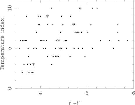
Figure 8: IPHAS $(r^{\prime}-i^{\prime})$ colour plotted against temperature index for all observed M-type stars with spectral type of M2 or later. The stars indicate the mean colour of each spectral type. A weak trend is noted between mean colour and temperature index.

There are 109 O-rich sources amongst our sample of 139 sources with LIRIS spectra. 31 of these show no evidence for TiO or VO features but do show CO bands. These have all been classified as type K0-M2. Some of these sources may be of later type but are unidentifiable because of the low transmission around 0.92 $\mu$m and the resulting inability to accurately remove the telluric absorption and identify any underlying features. Wright et al. (2008) estimated that K-type giants were unlikely to significantly contribute to the ERSO region because of their bluer intrinsic colours and lower luminosities. This could suggest that these unclassified sources are of early-to-mid M-type, but that the necessary spectral features to classify them as such are unavailable.

Of the remaining 78 sources, 45 show clear VO bands indicating they are of type M6 or later. This high fraction of late-type stars supports our use of the “extremely-red” region of the IPHAS colour-colour diagram to select such late-type sources for our spectral library. The M-type stars show an even distribution across the colour-colour plane in Figure 1. Figure 8 shows the $(r^{\prime}-i^{\prime})$ colours of all observed M-type stars with spectral types of M2 or later (earlier types are not included because of the large errors associated with determining spectral types from their relatively featureless spectra). A weak trend between $(r^{\prime}-i^{\prime})$ colour and spectral type does exist, though the spread is large and influenced by small number statistics. It is worth noting that the reddest source at each spectral type increases almost linearly from M2 to M6. This is most likely due to a combination of intrinsic colour and the fact that sources of later spectral type will be more luminous (therefore likely to be more distant and experience greater interstellar reddening) and may have undergone more mass loss (therefore have greater circumstellar reddening).

4.1.1 Emission-line sources

We searched for emission-lines in all our spectra, particularly for lines from the Paschen series found in the near-IR, e.g. P$\beta$ at 1.282 $\mu$m and P$\gamma$ at 1.094 $\mu$m. Mira variables are known to exhibit phase-dependent emission-lines in the spectra due to shocks in their atmospheres from stellar pulsations (e.g. Hinkle & Barnes, 1979). We observe emission lines in six of our spectra, three of which are oxygen-rich and three are S-type stars. Of the four stars with emission lines and for which temperature class information is available, all are of type M7 (or equivalent) or later suggesting that later type stars experience more shocks in their atmospheres. Since these shocks are thought to be due to stellar pulsations, this supports the belief that pulsations are stronger and more regular in stars of later spectral-type. The $(r^{\prime}-$H$\alpha)$ colours of all these sources are not particularly large, supporting the suggestion by Wright et al. (2008) that the 2 yr separation between IPHAS photometric measurements and these spectroscopic observations is longer than the temporary nature of these spectral features (likely to be less than the pulsation period of the star, Bessell et al., 1996).

The object with the strongest Paschen $\beta$ emission line is ERSO 27 (V890 Cas) which has $(r^{\prime}-$H$\alpha)=1.02$ and whose spectrum is shown in Figure 9. While it does not have a particularly high $(r^{\prime}-$H$\alpha)$ colour, it is an S-type star, which were shown by Wright et al. (2008) to have lower $(r^{\prime}-$H$\alpha)$ colours compared to O-rich stars, and so the effects of this and an H$\alpha$ emission line may be cancelling each other out.

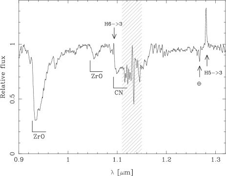
Figure 9: LIRIS $J$ band spectrum of ERSO 27. The spectrum has been corrected for telluric absorption (affected region marked) and divided by an adopted continuum. Molecular features typical of S-type stars are shown, as are the Paschen $\beta$ and $\gamma$ emission lines.

4.2 S-type and carbon stars

We find 22 S-type stars and 5 carbon stars in our spectral library. More than half of the S-type stars show no evidence for O-rich features, which gives them abundance indices of 6 or more (Keenan & Boeshaar, 1980). We find only 1 S-type star with an abundance index $\leq 2$, which we attribute to the difficulty in identifying the weak S-type features in these sources against the stronger O-rich features. A small number of O-rich stars may therefore have been mis-classified as such. There is a notable concentration of S-type stars towards lower $(r^{\prime}-$H$\alpha$) colours, supporting the trend originally noted by Wright et al. (2008), while the carbon stars show intermediate colours between the O-rich and S-type stars (an effect commented on by Drew et al., 2005). The reason for these colours is that in O-rich stars TiO features cause a falsely low continuum in the $r^{\prime}$ band, while the H$\alpha$ filter excludes these features resulting in a large ($r^{\prime}-$H$\alpha$) colour. S-type stars however have weaker ZrO features across the $r^{\prime}$ filter and a ZrO feature coincident with the H$\alpha$ filter, causing absorption resulting in a much lower ($r^{\prime}-$H$\alpha$) colour (see Figure 19 of Wright et al., 2008, for spectral examples of this effect).

To illustrate this effect we show in Figure 10 the ($r^{\prime}-$H$\alpha$) colour as a function of the abundance index used to classify S-type stars. Despite the small number of sources we note a clear trend for stars with a higher abundance index to have smaller ($r^{\prime}-$H$\alpha$) colours. We explain this trend as due to the waning strength of the TiO features that give rise to high ($r^{\prime}-$H$\alpha$) colours and the growing strength of ZrO features that give rise to low ($r^{\prime}-$H$\alpha$) colours. The minimum ($r^{\prime}-$H$\alpha$) colour appears to occur at an abundance index of 6 – 8, the stage where ZrO-dominated spectra shift to those dominated by the sodium D lines. It should be noted however that this relationship is only based on sources in the ERSO region of the IPHAS colour-colour plane and does not consider less reddened sources. It also does not consider any influence on the ($r^{\prime}-$H$\alpha$) colour of sources based on their ($r^{\prime}-i^{\prime}$) colour, for which the giant branch shows a clear gradient (e.g. Drew et al., 2005; Wright et al., 2008). O-rich sources with lower $(r^{\prime}-i^{\prime})$ colours will have lower ($r^{\prime}-$H$\alpha)$ colours and therefore a more accurate relationship on the $(r^{\prime}-$H$\alpha$) deficit must be determined as a function of the $(r^{\prime}-i^{\prime})$ colour.

The abundance index was considered by Keenan & Boeshaar (1980) to be a good indicator of the C/O ratio. However, the ZrO and TiO bands that determine the abundance index are dependent on the Zr/Ti ratio and the photospheric temperature as well (e.g. Zijlstra et al., 2004; García-Hernández et al., 2007). It had been thought that the Zr/Ti ratio might scale with the C/O ratio (Scalo & Ross, 1976), because both carbon and $s$-process elements are dredged to the surface during mixing events on the AGB. However a direct relationship has not been conclusively established (Vanture & Wallerstein, 2002) and the two mixing rates may be different or the ratios start from different initial values. If this were the case two scenarios would arise where C/O exceeds unity either after or before the Zr/Ti ratio reaches the level where ZrO bands outweigh TiO bands. In the former situation we would expect to see evolution follow the M-S-C sequence, with the S-type phase lasting until C/O exceeds unity. In the latter case the star might evolve straight from O-rich to C-rich without an S-type phase, potentially passing through a phase where all the C and O is tied up in CO and only sulphides are visible. A source such as ERSO105 with strong CO bands and no identifiable O-rich, S-type or C-rich features might be an example of such an object.

Figure 10: IPHAS $(r^{\prime}-$H$\alpha)$ colour plotted against the Keenan & Boeshaar (1980) abundance index for all carbon and S-type stars. Though carbon stars are not fully included on the scale of Keenan & Boeshaar (1980), we have included them here with an abundance index $\geq$10 to represent the chemical evolution of an evolved star. O-rich stars have an abundance indices of $\leq 1$ and are not shown on this figure. The trend of increasing $(r^{\prime}-$H$\alpha)$ colour with increasing $(r^{\prime}-i^{\prime})$ colour is also not considered in this figure.

4.2.1 Extrinsic and intrinsic S-type stars

A small subset of S-type stars (now dubbed extrinsic S stars) are believed to acquire their Zr not from the third dredge-up (as is typical for AGB stars) but from mass-transfer from an evolved binary companion during an earlier evolutionary phase (Jorissen & Mayor, 1988). When the star later evolved onto the red giant branch (RGB), ZrO was able to form. Extrinsic and intrinsic (true AGB stars) S-type stars were originally separated by studying lines from the unstable element Tc that are observed in the atmospheres of AGB stars (following nucleosynthesis and the third dredge-up) but not in the less-evolved RGB stars where it has decayed (Brown et al., 1990). To determine if the S-type stars identified in this work are intrinsic or extrinsic, we have utilised the near- and mid-infrared colour-colour diagrams presented by Yang et al. (2006). They found that the $(K-\mathrm{[12]})$ vs $(J-\mathrm{[25]})$ colour-colour diagram could be used to separate the two types of stars, approximately separating the RGB stars with little or no circumstellar material from the more evolved AGB stars with considerable circumstellar material. We combined 2MASS (Two-Micron All Sky Survey, Skrutskie et al., 2006) near-IR photometry with either IRAS (Infrared Astronomical Satellite, Neugebauer et al., 1984) or MSX (Midcourse Space Experiment, Egan & Price, 1996) mid-IR fluxes as per Wright et al. (2008). We find suitable associations for 18 of the 22 S-type stars and that all have colours placing them in the region of the near- and mid-IR colour-colour diagram characterised by intrinsic S-type stars. It is likely that our colour selection criteria for these spectra has preferentially selected the redder and more luminous AGB stars over red giant branch stars and has therefore selected intrinsic S-type stars over extrinsic types.

4.3 Notes on individual sources

The S-type star ERSO 24 lies 8.6^′′ from the variable star EI Per, which Bidelman (1987) identified from infrared plates as a Mira of spectral type M8. Our spectra show very strong ZrO bands (see Figure 3) and we find no evidence for O-rich features, including the H-band OH lines. IPHAS images of ERSO 24 show no other sources within 30^′′ with reddened colours. Despite the difference in spectral type between EI Per and ERSO 24 we find no other candidates for EI Per in the IPHAS images so assume that the two are the same star. The star has either undergone a recent abundance change from O-rich to S-type or the previous unverifiable spectral type identification was inaccurate.

ERSO 60 is located 6.4^′′ from an IRAS source that Cohen (1995) suggested could be a Wolf-Rayet candidate based on its position in the IRAS two colour diagram. An inspection of IPHAS images reveal no other highly reddened sources in the vicinity, suggesting that the IRAS source is most likely associated with ERSO 60, the spectra of which indicate it is certainly a C-rich AGB star.

ERSO 80 was classified by Stephenson (1990) as an S-type star, who noted that the object had no TiO bands, weak LaO bands and was quite red. Our spectra do not show any TiO or ZrO features, but do show moderate CN bands at 1.088 $\mu$m, as well as a very clean $H$-band CO spectrum with no OH bands, both indicative of a near unity C/O ratio. There is no evidence for any bands of C₂, which can appear for C/O$>1$, so our spectral classification is limited to an abundance class of 8, which Keenan & Boeshaar (1980) define as a star having no ZrO or C₂, and C/O $\sim 1$. The deep CO bands and the presence of LaO, which is only thought to be visible for T${}_{eff}<2800$ K, indicates a relatively cool photosphere and a temperature class around $9\pm 2$. Therefore we assign ERSO 80 a spectral classification of S9/8 on the S-type classification system, or SC9/8 since it is an SC-type star.

ERSO 136 is listed in the General catalog of galactic carbon stars (Alksnis et al., 2001), but its position in the IRAS colour-colour diagram suggests O-rich circumstellar chemistry, as noted by Chen et al. (2003) who suggested the star is actually O-rich. IRAS low-resolution spectra (Omont et al., 1993) show no evidence for silicate dust features and our spectra contain weak CN lines in the J- and H-bands, which indicates a potentially C-rich object. The lack of both the 1.77 $\mu$m C₂ band and very strong CO bands indicates that the C/O ratio is near unity. If this source has only recently become C-rich it may explain its ambiguous mid- and far-infrared colours and spectra.

5 Conclusions

We have presented near-IR spectra of 139 AGB stars that have been classified by comparison with existing spectral libraries. Our spectral library covers the full range of O-rich, S-type and carbon stars, with a significant number of very late-type sources in all chemical types. This was achieved by selecting sources from the extremely red region of the IPHAS colour-colour plane, which has been shown to be dominated by late-type AGB stars. Classification of late K-type and early M-type stars was not possible due to the lack of clear classification diagnostics at our resolution for these sources.

The spectral library also includes a significant fraction of S-type stars, which have been classified by temperature index and abundance index where possible. We find a strong correlation between the IPHAS $(r^{\prime}-$H$\alpha)$ colour and the C/O abundance index for S-type and carbon stars. Combined with photometry in the near-IR (e.g. Cioni & Habing, 2003), this relation could be used to separate O-rich, S-type and carbon stars based on photometry alone. Given the recent generation of optical and near-IR photometric surveys across the Galactic Plane, data are available to provide a broad identification of AGB-star chemistries across much of the Galaxy from the solar neighbourhood outward. Since the fraction of O-rich, S-type and carbon stars is a known indicator of metallicity, this could be used to trace the metallicity gradient in the outer Galactic disk. Further spectra will be necessary to refine this relationship and determine its dependence on the IPHAS $(r^{\prime}-i^{\prime})$ colour.

6 Acknowledgments

This work is based in part on observations made with the Isaac Newton Telescope and the William Herschel Telescope, operated on the island of La Palma by the Isaac Newton Group. Observations on the WHT were obtained through an International Time Programme, awarded to the IPHAS collaboration. It also partly makes use of data products from 2MASS, IRAS and MSX, which are jointly run by the Infrared Processing and Analysis Center and the California Institute of Technology, and funded by the National Aeronautics and Space Administration and the National Science Foundation. This research has made use of the Simbad database, operated at CDS, Strasbourg, France, and IRAF, operated by the Association of Universities for the Research in Astronomy, Inc., under cooperative agreement with the National Science Foundation. NJW was supported by a PPARC Studentship and a Smithsonian Astrophysical Observatory Pre-doctoral Fellowship.

References

- Acosta Pulido et al. (2003) Acosta Pulido J. A., Ballesteros E., Barreto M., et al., 2003, The Newsletter of the Isaac Newton Group of Telescopes (ING Newsl.), Issue no. 7, p. 15-16.
- Alksnis et al. (2001) Alksnis A., Balklavs A., Dzervitis U., Eglitis I., Paupers O., Pundure I., 2001, Baltic Astronomy, 10, 1
- Aoki et al. (1998) Aoki W., Tsuji T., Ohnaka K., 1998, A&A, 340, 222
- Bessell et al. (1996) Bessell M. S., Scholz M., Wood P. R., 1996, A&A, 307, 481
- Bidelman (1987) Bidelman W. P., 1987, Information Bulletin on Variable Stars, 2993, 1
- Brett (1990) Brett J. M., 1990, A&A, 231, 440
- Brown et al. (1990) Brown J. A., Smith V. V., Lambert D. L., Dutchover E. J., Hinkle K. H., Johnson H. R., 1990, AJ, 99, 1930
- Chen et al. (2003) Chen P.-S., He J.-H., Wang X.-H., 2003, Chinese Astronomy and Astrophysics, 27, 147
- Cioni & Habing (2003) Cioni M.-R. L., Habing H. J., 2003, A&A, 402, 133
- Cohen (1995) Cohen M., 1995, ApJS, 100, 413
- Davis & Hammer (1981) Davis S. P., Hammer P. D., 1981, ApJ, 250, 805
- Drew et al. (2005) Drew J. E., Greimel R., Irwin M. J., et al., 2005, MNRAS, 362, 753
- Egan & Price (1996) Egan M. P., Price S. D., 1996, AJ, 112, 2862
- García-Hernández et al. (2007) García-Hernández D. A., García-Lario P., Plez B., Manchado A., D’Antona F., Lub J., Habing H., 2007, A&A, 462, 711
- Goebel et al. (1981) Goebel J. H., Bregman J. D., Witteborn F. C., Taylor B. J., Willner S. P., 1981, ApJ, 246, 455
- González-Solares et al. (2008) González-Solares E. A., Walton N. A., Greimel R., et al., 2008, MNRAS, 388, 89
- Hachtouki & Auwera (2002) Hachtouki R. E., Auwera J. V., 2002, JQSRT, 216, 355
- Hinkle & Barnes (1979) Hinkle K. H., Barnes T. G., 1979, ApJ, 234, 548
- Hinkle et al. (1989) Hinkle K. H., Lambert D. L., Wing R. F., 1989, MNRAS, 238, 1365
- Hunaerts (1967) Hunaerts J., 1967, ApJL, 149, L31+
- Ichikawa (1981) Ichikawa T., 1981, PASJ, 33, 107
- Iyengar & MacConnell (1998) Iyengar K. V. K., MacConnell D. J., 1998, A&AS, 133, 201
- Jonsson et al. (1992) Jonsson J., Launila O., Lindgren B., 1992, MNRAS, 258, 49
- Jorissen & Mayor (1988) Jorissen A., Mayor M., 1988, A&A, 198, 187
- Joyce (1998) Joyce R. R., 1998, AJ, 115, 2059
- Joyce et al. (1998) Joyce R. R., Hinkle K. H., Wallace L., Dulick M., Lambert D. L., 1998, AJ, 116, 2520
- Kazarovets et al. (2003) Kazarovets E. V., Kireeva N. N., Samus N. N., Durlevich O. V., 2003, Information Bulletin on Variable Stars, 5422, 1
- Keenan (1993) Keenan P. C., 1993, PASP, 105, 905
- Keenan & Boeshaar (1980) Keenan P. C., Boeshaar P. C., 1980, ApJS, 43, 379
- Kleinmann & Hall (1986) Kleinmann S. G., Hall D. N. B., 1986, ApJS, 62, 501
- Kun (1987) Kun M., 1987, Information Bulletin on Variable Stars, 3106, 1
- Kurucz (1979) Kurucz R. L., 1979, ApJS, 40, 1
- Kwok et al. (1997) Kwok S., Volk K., Bidelman W. P., 1997, ApJS, 112, 557
- Lambert & Clegg (1980) Lambert D. L., Clegg R. E. S., 1980, MNRAS, 191, 367
- Lançon et al. (2007) Lançon A., Hauschildt P. H., Ladjal D., Mouhcine M., 2007, A&A, 468, 205
- Lançon & Wood (2000) Lançon A., Wood P. R., 2000, A&AS, 146, 217
- Le Squeren et al. (1992) Le Squeren A. M., Sivagnanam P., Dennefeld M., David P., 1992, A&A, 254, 133
- Loidl et al. (2001) Loidl R., Lançon A., Jørgensen U. G., 2001, A&A, 371, 1065
- Manchado et al. (2004) Manchado A., Barreto M., Acosta-Pulido J., et al., 2004, in Moorwood A. F. M., Iye M., eds, Ground-based Instrumentation for Astronomy. Edited by Alan F. M. Moorwood and Iye Masanori. Proceedings of the SPIE, Volume 5492, pp. 1094-1104 (2004). First light for LIRIS (long-slit intermediate-resolution infrared spectrograph). pp 1094–1104
- Matsuura et al. (1999) Matsuura M., Yamamura I., Murakami H., Freund M. M., Tanaka M., 1999, A&A, 348, 579
- Meyer et al. (1998) Meyer M. R., Edwards S., Hinkle K. H., Strom S. E., 1998, ApJ, 508, 397
- Neugebauer et al. (1984) Neugebauer G., Habing H. J., van Duinen R., et al., 1984, ApJL, 278, L1
- Omont et al. (1993) Omont A., Loup C., Forveille T., Te Lintel Hekkert P., Habing H., Sivagnanam P., 1993, A&A, 267, 515
- Origlia et al. (1993) Origlia L., Moorwood A. F. M., Oliva E., 1993, A&A, 280, 536
- Phillips (1969) Phillips J. G., 1969, ApJ, 157, 449
- Phillips et al. (1979) Phillips J. G., Davis S. P., Galehouse D. C., 1979, ApJ, 234, 401
- Querci et al. (1974) Querci F., Querci M., Tsuji T., 1974, A&A, 31, 265
- Ramirez et al. (1997) Ramirez S. V., Depoy D. L., Frogel J. A., Sellgren K., Blum R. D., 1997, AJ, 113, 1411
- Rosino et al. (1976) Rosino L., Bianchini A., di Martino D., 1976, A&AS, 24, 1
- Rothman et al. (2009) Rothman L. S., Gordon I. E., Barbe A., Benner D. C., et al., 2009, JQSRT, 110, 533
- Scalo & Ross (1976) Scalo J. M., Ross J. E., 1976, A&A, 48, 219
- Schiavon & Barbuy (1999) Schiavon R. P., Barbuy B., 1999, ApJ, 510, 934
- Skiff (1999) Skiff B. A., 1999, Information Bulletin on Variable Stars, 4678, 1
- Skrutskie et al. (2006) Skrutskie M. F., Cutri R. M., Stiening R., Weinberg M. D., Schneider S., Carpenter J. M., Beichman C., 2006, AJ, 131, 1163
- Smith & Lambert (1990) Smith V. V., Lambert D. L., 1990, ApJL, 361, L69
- Stephenson (1990) Stephenson C. B., 1990, AJ, 100, 569
- Stephenson (1992) Stephenson C. B., 1992, Information Bulletin on Variable Stars, 3800, 1
- Tanaka et al. (2007) Tanaka M., Letip A., Nishimaki Y., Yamamuro T., Motohara K., Miyata T., Aoki W., 2007, PASJ, 59, 939
- Usatov & Nosulchik (2008) Usatov M., Nosulchik A., 2008, Open European Journal on Variable Stars, 87, 1
- Vanture & Wallerstein (2002) Vanture A. D., Wallerstein G., 2002, ApJ, 564, 395
- Wallace & Hinkle (1997) Wallace L., Hinkle K., 1997, ApJS, 111, 445
- Wallace et al. (2000) Wallace L., Meyer M. R., Hinkle K., Edwards S., 2000, ApJ, 535, 325
- Wright et al. (2008) Wright N. J., Greimel R., Barlow M. J., et al., 2008, MNRAS, 390, 929
- Yang et al. (2006) Yang X., Chen P., Wang J., He J., 2006, AJ, 132, 1468
- Zijlstra et al. (2004) Zijlstra A. A., Bedding T. R., Markwick A. J., et al., 2004, MNRAS, 352, 325