A High Fidelity Sample of Cold Front Clusters from the CHANDRA Archive

Abstract

This paper presents a sample of “cold front” clusters selected from the Chandra archive. The clusters are selected based purely on the existence of surface brightness edges in their Chandra images which are modeled as density jumps. A combination of the derived density and temperature jumps across the fronts is used to select nine robust examples of cold front clusters: 1ES0657-558, Abell 1201, Abell 1758N, MS1455.0+2232, Abell 2069, Abell 2142, Abell 2163, RXJ1720.1+2638, and Abell 3667. This sample is the subject of an ongoing study aimed at relating cold fronts to cluster merger activity, and understanding how the merging environment affects the cluster constituents. Here, temperature maps are presented along with the Chandra X-ray images. A dichotomy is found in the sample in that there exists a subsample of cold front clusters which are clearly mergers based on their X-ray morphologies, and a second subsample which harbor cold fronts, but have surprisingly relaxed X-ray morphologies, and minimal evidence for merger activity at other wavelengths. For this second subsample, the existence of a cold front provides the sole evidence for merger activity at X-ray wavelengths. We discuss how cold fronts can provide additional information which may be used to constrain merger histories, and also the possibility of using cold fronts to distinguish major and minor mergers.

1. Introduction

The hierarchical nature of structure formation is well understood theoretically (Press & Schechter, 1974; Lacey & Cole, 1993; Peebles, 1993; Springel et al., 2006) and well supported observationally (Smoot et al., 1992; Hernquist et al., 1996; Cole et al., 2005; Jeltema et al., 2005). At the present epoch, clusters of galaxies are the largest and most massive large-scale structures that are virialized and they are growing hierarchically through the gradual accretion of surrounding matter. Occasionally, two clusters of roughly equal mass fall together in a major merger, releasing around $10^{64}$ erg of gravitational potential energy during the merger process (Markevitch et al., 1999). To a degree, the majority of clusters exhibit evidence for merger activity. However it is the scale of the cluster mergers, i.e., the distinction between major mergers and the continuing minor mergers/infall of smaller subsystems, that is difficult to quantify. A gauge of merger activity capable of distinguishing major and minor mergers would greatly assist to understand mergers and their effects on clusters and their constituents.

A solution may be provided by high resolution X-ray observations with the Chandra observatory (Weisskopf et al., 2002). Among its first discoveries was the detection and characterization of the “cold front” phenomenon in the intracluster media (ICM) of Abell 2142 (Markevitch et al., 2000) and Abell 3667 (Vikhlinin et al., 2001a). Cold fronts reveal themselves as edge-like features in the Chandra images and are well modeled as contact discontinuities which form at the interface of cool, dense gas and hotter, more diffuse gas. Simulations show cold fronts can arise in more than one way during cluster mergers (Poole et al., 2006; Ascasibar & Markevitch, 2006). Broadly speaking, cold fronts can be separated into two general types: “remnant core” and “sloshing” (for a review see Markevitch & Vikhlinin, 2007).

Remnant core type cold fronts were first invoked to explain the origin of the cold fronts in Abell 2142 (Markevitch et al., 2000). In this case, the discontinuity occurs between the interface of an infalling subcluster’s cool core and the hotter ambient ICM of the main cluster. The subcluster’s core is bared to the hotter ICM after ram pressure stripping removes its less dense, lower pressure outer atmosphere during its passage through the main cluster. The cool core survives longest because, at first, it remains bound to the infalling dark matter core and, after separating from that, because of its high density. This explanation for Abell 2142’s cold fronts has since been abandoned in favor of a “sloshing” type mechanism (Markevitch & Vikhlinin, 2007). An excellent example of remnant core type cold front is observed in the Bullet cluster (1ES0657-558; Markevitch et al., 2002) while a similar mechanism acts to form cold fronts in the elliptical galaxies NGC 1404 and NGC 4552 (where the cold fronts are at the interface of the galaxy’s gas and the cluster ICM; Machacek et al., 2005, 2006). Furthermore, remnant core type cold fronts have also been seen in both idealized (Ascasibar & Markevitch, 2006; Poole et al., 2006; Springel & Farrar, 2007; Mastropietro & Burkert, 2008) and cosmological (Bialek et al., 2002; Nagai & Kravtsov, 2003; Onuora et al., 2003; Mathis et al., 2005) simulations of cluster mergers.

Gas “sloshing” came to the fore as an explanation for the existence of a cold front in the “relaxed” cluster Abell 1795 (Markevitch et al., 2001). These cold fronts occur when the stably stratified ICM is disturbed in such a way that the cool, dense gas residing in the cluster core is displaced from its position at the bottom of the gravitational potential well. The cold front is the contact discontinuity formed at the interface of the low entropy core gas and the higher entropy gas at larger radii. In most postulated scenarios, the disturbance is gravitational in nature with its origin in an infalling subcluster (e.g. Tittley & Henriksen, 2005; Ascasibar & Markevitch, 2006). However, there have been suggestions the disturbance may be a hydrodynamic phenomenon in the form of weak shocks or acoustic waves (Churazov et al., 2003; Fujita et al., 2004), while Markevitch et al. (2003b) suggest AGN explosions may be responsible, although the example of Hydra A used was later shown to be better interpreted as a weak shock (Nulsen et al., 2005). To date, the Ascasibar & Markevitch (2006) study provides the most comprehensive set of simulations for the sloshing scenario and show it is possible that the cold fronts observed in otherwise relaxed appearing clusters (based on their X-ray morphologies) can be produced by sloshing induced in relatively minor mergers. Currently, there is no observational evidence that the cold fronts in these relaxed appearing clusters are related to merger activity.

While cold fronts offer interesting insights into the physical properties of the ICM (e.g., Vikhlinin et al., 2001b; Churazov & Inogamov, 2004; Lyutikov, 2006; Markevitch & Vikhlinin, 2007; Xiang et al., 2007), it is how their presence relates to cluster merger activity, along with the tantalizing possibility of utilizing cold fronts as a gauge for cluster mergers, which provides the motivation for the study presented in this paper. The utilization of cold fronts as merger gauges becomes even more compelling when considering those clusters which appear to harbor relaxed X-ray morphologies—the existence of a cold front provides the only indication of ongoing merger activity at X-ray wavelengths. Much work has gone into studying cold front formation with simulations, but what has been lacking to date is a systematic study of the relationship between cold fronts and other dynamical indicators of cluster merger activity. The number of clusters observed by Chandra  to harbor cold fronts has grown significantly and now allows a representative sample to be assembled in order to perform such a study. To this end, this paper focuses on the selection of a sample of clusters with cold fronts in their Chandra  X-ray images. The selection criteria are designed to ensure that the high quality X-ray data shows an unambiguous cold front in each member of the sample.

To date, our goal of establishing whether there is a link between the presence of cold fronts in clusters and evidence of recent dynamical growth has been met, at least partially, in two cases, Abell 1201 (Owers et al., 2009b) and Abell 3667 (Owers et al., 2009a). In these studies, significant dynamical substructure was detected using spatial and redshift information provided by large samples of spectroscopically confirmed cluster member galaxies. In these clusters, the presence of a cold front is directly related to the presence of substructures, and thus ongoing merger activity. Future work will endeavor to go one step further and study the galaxy properties within the cold front clusters.

The outline of this paper is as follows. In Section 2 the procedure for selecting cold front clusters is presented. In Section 3 the technique used to generate projected temperature maps for each cold front cluster is described. In Section 4 the Chandra  X-ray images and temperature maps for the clusters in the cold front sample are presented, along with a brief description of the X-ray properties and evidence for merger activity from the literature. In Section 5, the results and sample are discussed. In Section 6 summary and conclusions are presented.

2. Sample selection criteria

2.1. Initial Selection

To ensure selection of only the best defined cold front clusters, the following criteria were set. The data must be of high enough quality that statistically robust measurements of density and temperature can be made on either side of the edge in surface brightness for characterization. The bulk of the cluster X-ray emission must be captured on the Chandra  chips, whilst resolution and cosmological surface brightness dimming affects must be minimized. Clearly, the cluster must also exhibit an edge in the surface brightness, indicating the existence of a density discontinuity caused by a cold front.

The initial sample was selected from those clusters with publicly available data within the Chandra  archive (as of July 2006) and the preceding conditions were imposed as the following quantitative criteria:

• a total Chandra ACIS-I and/or ACIS-S exposure time exceeding 40 ks;

• cluster redshift in the range $0.05\leq z\leq 0.3$;

• a significant edge in the X-ray surface brightness.

The density discontinuities caused by cold fronts are generally quite visible in the Chandra images, and their existence is easily verified by the observation of edges and compression of isophotal contours overlaid onto the images. Thus, for each Chandra data set meeting the first three selection criteria, the 0.5 – 7 keV band image was scrutinized for edge-like features and regions of compressed isophotes. It is noted that the morphology of the X-ray emission was not considered during the selection process, nor were any clusters selected based on prior knowledge of a cold front in their ICM. The significance of the density discontinuity was quantified by modeling the surface brightness across the edge with a broken power law density model (see Appendix A). The surface brightness edge must also be reasonably sharp, i.e., in order to be classified as a front, they must be reasonably well fitted by the density jump model.

This model was used to further cull the sample and is presented in Appendix A. A description of the method used to fit the model to the data follows.

2.2. Fitting the surface brightness across the edges

Corresponding to the broken power law density model, the surface brightness model given in Equation A4 was incorporated into the Sherpa fitting software, which is part of the Chandra Interactive Analysis of Observations (CIAO; version 3.4 is used here) package. Point sources were identified using the CIAO WAVDETECT tool and removed for fitting. The images were restricted to the energy range 0.5 – 7 keV, so that background and instrument effects were minimized, whilst still allowing enough source photons to obtain good fits to the models. Where possible, separate observations had their data and exposure maps co-added prior to fitting. The background count rates for Chandra observations is known to change with time, and also to differ between the ACIS-S and ACIS-I arrays. For these reasons, observations taken at significantly different times, or taken using different chips were not co-added, but were simultaneously fitted with separate background components. The fit was restricted to regions where there are edges (the blue regions shown in the top left panels of Figures 2 through 10), and the initial inputs for the center of the spheroid, the ellipticity, $\epsilon$, the orientation angle, $\theta$, and the radius at which the edge occurs, $R_{f}$, were obtained by overlaying an elliptical region that best approximated the surface brightness contours across the edge. The center of curvature was not necessarily the position of the X-ray centroid of the cluster, and the semimajor axis of the ellipse, $\theta$, was oriented to bisect the edge. Since the center, $\theta$ and $R_{f}$ are highly degenerate, the center and $\theta$ were fixed to those values determined from the manually fitted ellipse and only $R_{f}$ was determined directly from the fit. A fixed, uniform background component was added to the model during fitting. The background was determined by fitting the entire Chandra  observed area using one or two beta models plus a constant component. The beta model/s account for the cluster emission, and the constant component for the background. We note that this constant background component does not correctly account for the unvignetted instrumental background. This does not affect our results because: a) the edges are found in regions where the cluster emission is dominant and b) the quantity of interest is the break in the surface brightness profile which is insensitive to both the background level and to small changes in the background slope (when the background does not dominate). Each model was multiplied by the exposure map, generated using the CIAO MKINSTMAP, ASPHIST and MKEXPMAP tools, which account for instrumental effects such as vignetting, Quantum Efficiency (QE), QE nonuniformity, bad pixels, dithering and effective area.

After fitting the density model (Appendix A4), the sample was limited to include only those clusters where the density jump exceeded a factor of 1.5 at the lower limit of the $90\%$ confidence interval. The confidence intervals were estimated using the PROJECTION tool in Sherpa, which varies the parameter of interest along a grid of values whilst allowing adjustable model parameters to settle to their new best-fitted values. This criterion eliminated several clusters with clearly visible surface brightness edges from the sample. Thus, any detectable cold fronts in clusters meeting the other selection criteria above that were missed in the search of the archive are unlikely to have density jumps exceeding a factor of 1.5. The 11 clusters which meet the above criteria, along with the parameters for the fits, are presented in Table 1. The corresponding surface brightness distributions with the surface brightness profiles for the best fitting density models overlaid are plotted in Figure 1. Interestingly, Abell 2142 is the only one of the 11 clusters to require a significant ellipticity in the fits. It is noted that density jumps determined from the surface brightness fits do not depend on the curvature of the front ($\epsilon_{\zeta}$ in Appendix A4), but they do depend on the assumption that the density profiles can be expressed in terms of the same coordinate ($r$ in equation A1) on both sides of the front. The Chandra  Observation Identification number, cluster center and redshift are presented in Table 2 along with global spectral properties (Section 2.3.1). To confirm that these structures are cold fronts, temperature measurements on each side of the front are required (see Section 2.3.2).

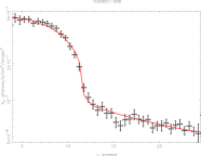
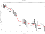
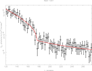
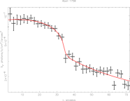
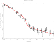
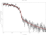
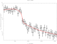
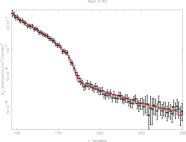
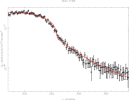
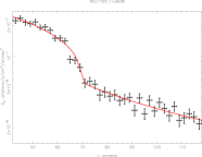
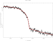
Figure 1.— Surface brightness profiles across the edges (black points with error bars) with the surface brightness for the best fitting density model plotted in red. The corresponding model parameters can be found in Table 1. The clusters shown are (from left to right, top row through bottom row) 1ES0657-558, Abell 665, Abell 1201, Abell 1758, MS1455.0+2232, Abell 2034, Abell 2069, Abell 2142, Abell 2163, RXJ1720.1+2638 and Abell 3667.

Table 1Parameters of the density model fits for the 11 clusters with significant density discontinuities.

Cluster	(x,y)	$\theta(\Delta\theta)$	$R_{f}$	$\epsilon$	$A_{1}$	$\alpha_{1}$	$A_{2}$	$\alpha_{2}$
	(J2000)	(deg)	(kpc)		$(10^{-8})$		$(10^{-8})$
1ES0657-558	104.58518, -55.941469	0 (310 - 50)	$53_{-0.2}^{+0.4}$	0	$22.7_{-1.4}^{+1.5}$	$0.0_{-0.1}^{+0.1}$	$2.6_{-0.4}^{+0.4}$	$0.9_{-0.1}^{+0.1}$
Abell 665	127.74663, 65.842256	252 (233 - 270)	$192_{-3}^{+5}$	0	$3.6_{-0.1}^{+0.1}$	$0.7_{-0.4}^{+0.4}$	$0.8_{-0.3}^{+0.3}$	$1.0_{-0.2}^{+0.2}$
Abell 1201	168.2197, 13.4509	254 (240-267)	$503_{-8}^{+4}$	0	$2.0_{-0.3}^{+0.3}$	$1.0_{-0.3}^{+0.4}$	$0.4_{-0.1}^{+0.2}$	$1.3^{+0.3}_{-0.2}$
Abell 1758N	203.1603, 50.5575	98 (45-150)	$150_{-2}^{+2}$	0	$3.9_{-0.4}^{+0.4}$	$-0.1_{-0.1}^{+0.1}$	$1.1_{-0.2}^{+0.2}$	$1.1_{-0.1}^{+0.1}$
MS1455.0+2232	224.3125, 22.3427	132 (114-150)	$150_{-1}^{+1}$	0	$13.2_{-1.3}^{+1.4}$	$1.2_{-0.2}^{+0.2}$	$3.4_{-0.8}^{+0.9}$	$1.6_{-0.2}^{+0.3}$
Abell 2034	227.53396, 33.495151	120 (104-126)	$521_{-2}^{+1}$	0	$3.7_{-0.2}^{+0.2}$	$-0.4_{-0.1}^{+0.1}$	$0.7_{-0.1}^{+0.1}$	$2.8_{-0.2}^{+0.2}$
Abell 2069	231.12201, 29.994898	25 (3 - 46)	$383_{-3}^{+4}$	0	$1.1_{-0.2}^{+0.2}$	$-1.3_{->0.2}^{+0.5}$	$0.3_{-0.1}^{+0.1}$	$1.8_{-0.2}^{+0.2}$
Abell 2142	239.5863, 27.226989	40 (10 - 100)	$360_{-1}^{+3}$	$0.36_{-0.01}^{+0.01}$	$7.0_{-0.4}^{+0.1}$	$0.9_{-0.03}^{+0.1}$	$1.8_{-0.1}^{+0.1}$	$1.3_{-0.1}^{+0.04}$
Abell 2163	243.97508, -6.1117719	315 (310-320)	$856_{-2}^{+2}$	0	$18.3_{-0.6}^{+0.7}$	$-0.4_{-0.1}^{+0.1}$	$5.2_{-0.4}^{+0.4}$	$3.8_{-0.1}^{+0.1}$
RXJ1720.1+2638	260.03982, 26.624822	234 (205 - 263)	$190_{-1}^{+2}$	0	$10.1_{-0.9}^{+0.8}$	$0.4_{-0.2}^{+0.2}$	$2.4_{-0.4}^{+0.3}$	$1.4_{-0.1}^{+0.1}$
Abell 3667	303.14776, -56.819424	230 (222 - 238)	$411_{-1}^{+0.3}$	0	$4.4_{-0.1}^{+0.2}$	$-0.7_{-0.1}^{+0.1}$	$0.6_{-0.1}^{+0.1}$	$1.5_{-0.1}^{+0.2}$

Note. — For a description of the density model parameters $A_{1},\,A_{2},\,\alpha_{1}$ and $\alpha_{2}$, see Appendix A.

2.3. Preparation of data for Spectral measurements

Since the ACIS chips on board Chandra  record both spatial and energy information for incident photons, it is possible to extract spatially resolved spectra from the images. As for all astrophysical spectral observations, the data need to be processed carefully in order to exclude events not related to the source (e.g. cosmic rays), calibrate the energy and also to account for the backgrounds. Here, the procedure used to prepare the data for spectral extraction is described.

The archived Chandra pipeline data were reprocessed starting with the level 1 event files and using CIAO version 3.4 with the Calibration Database version 3.4.0. Observation specific bad pixel files were produced and applied, as were the latest gain files. Observations taken at focal plane temperatures of $-120^{\circ}$C had corrections applied for charge transfer inefficiency and time dependent gain. Where observations were taken in VFAINT telemetry mode, the more thorough VFAINT mode of cleaning was used for improved rejection of cosmic rays. Only events with ASCA grades of 0, 2, 3, 4 and 6 were retained during the analysis.

Backgrounds were taken from the blank sky observations appropriate for the epoch of observation. Since the blank sky backgrounds are taken from observations with low Galactic foregrounds and low soft X-ray brightness, the soft X-ray flux was checked in the vicinity of each cluster using the ROSAT all sky R45 count rates, and compared to the blank sky background rates. If the R45 fluxes were anomalous (e.g. MS1455.0+2232, Abell 2163 and Abell 3667), a region relatively free from cluster emission was selected and spectra extracted to model the soft component using a single or double MEKAL model at zero redshift (see e.g. Markevitch et al., 2003a). The soft component was included in all spectral analyses, with the normalization weighted by a geometric factor to allow for the different extraction areas. The background and source data were processed using the same calibration files, bad pixel files and background filtering, with the backgrounds being reprojected to match the observations.

To match the blank sky backgrounds, the observations were filtered for periods of high cosmic ray background caused by flares. The point sources and regions containing cluster emission were excluded and a light curve was extracted and binned in time intervals of 259 seconds in the energy range 0.3-10 keV for the ACIS-I array, whilst the ACIS-S array data were binned in intervals of 1037 seconds in the energy range 2.5-6 keV. The light curve was analyzed in Sherpa using the lc_clean.sl script and only periods where the background count rate was within 20% of the quiescent rate were included.

During the spectral analysis of Abell 1758N, it was necessary to account for a soft flare present for the duration of the observation. The method described in David & Kempner (2004) was used, whereby the flare shape was modeled in PHA space in a region relatively free from cluster emission, using the cutoffpl model in XSPEC with power law index = 0.15 and an exponential cut off at E=5.6 keV, with the normalization allowed to vary. The flare model was then incorporated into spectral fits with all parameters fixed and the normalization set to its best fitted value from above multiplied by a geometric factor correcting for the different extraction region areas.

2.3.1 Global Temperatures

To obtain a picture of the overall thermal properties of the 11 clusters, global temperatures and metallicities were measured. Where possible, a region covering the majority of the cluster emission was selected and spectra were extracted using the CIAO DMEXTRACT tool, with point sources detected with WAVDETECT excised. The regions within which the spectra were extracted are shown in red in the X-ray images presented in the top left panels of Figures 2 through 10. The CIAO tool MKWARF was used to create auxiliary response files (ARF), which account for spatial variations in quantum efficiency (QE), effective area and also the temporal dependence of the effective area due to molecular contamination on the optical blocking filter. For observations performed with a focal plane temperature of $-120^{\circ}$C, the CIAO MKACISRMF tool was used to create redistribution matrix files (RMF), while MKRMF was used for this purpose for observations performed at $-110^{\circ}$C. Since the responses depend on the chip position, they are calculated in regions in chip coordinates and are weighted by the 0.5 – 2 keV brightness of the cluster within that region, with the final ARF and RMFs being count weighted. For clusters with multiple observations where a more recent, significantly longer exposure was available, the earlier, shorter observations were excluded from the global temperature measurement.

The spectra were fitted in the 0.5-9.8 keV range for ACIS-S observations and 0.6-9.8 keV for ACIS-I observations in XSPEC (Arnaud, 1996) using a MEKAL model (Mewe et al., 1985, 1986; Kaastra, 1992; Liedahl et al., 1995), for a hot, diffuse, single temperature plasma, multiplied by WABS, a photo-electric absorption model accounting for Galactic absorption, where the neutral hydrogen column density is initially fixed to the Galactic value provided by Dickey & Lockman (1990). The spectra were binned so that each energy bin contains at least 30 counts and the normalization, temperature and abundance were fitted in the first iteration, with the column density fixed to the Galactic value. The metal abundances are measured relative to the solar photospheric values of Anders & Grevesse (1989). Where the data allow, the column density was then freed and the data re-fitted, with the best fitting results along with their associated $90\%$ errors presented in Table 2. For the clusters 1ES0657-558, Abell 2142, Abell 2163 and Abell 3667 the measured $N_{\rm H}$ values are inconsistent with the Galactic values within the $90\%$ confidence limits, although they are consistent with values measured by others in the literature (e.g. Govoni et al., 2004; Markevitch et al., 2000; Vikhlinin et al., 2001a). In the clusters Abell 665 and RXJ1720.1+2638, the $N_{\rm H}$ values are also inconsistent with Galactic values, however the temperature and abundance measurements appear to be relatively unaffected and they are consistent with previously measured values (Mazzotta et al., 2001; Govoni et al., 2004, for RXJ1720.1+2638  and Abell 665, respectively.). The LUMIN function in XSPEC was used to determine the integrated, unabsorbed X-ray luminosity from the best fitting model in the energy range 0.5-9.8 keV, with the results presented in Table 2.

Table 2Clusters with density jumps exceeding 1.5 at the lower $90\%$ confidence interval. The exposure times presented in parentheses are the cleaned exposure times used to generate the temperature maps. The $N_{\rm H}$ values presented in parentheses are the galactic values.

Cluster	ObsId	Exposure	RA	DEC	Redshift	$kT$	$Z$ ($Z\odot$)	$L_{\rm X}$	$N_{\rm H}$
		(ks)	(J2000)	(J2000)		(keV)		($10^{44}\rm\ erg/s$)	$\times 10^{20}$
1ES0657-558	3184, 4984, 4985,	551 (535)	06:58:27	-55:56:47	0.296	$14.7^{+0.3}_{-0.3}$	$0.32^{+0.03}_{-0.02}$	43.0	$3.7^{+0.3}_{-0.3}$(6.53)
	4986, 5355, 5356
	5357, 5358, 5361
Abell 665	531, 3586	40 (35)	08:30:45	65:52:55	0.182	$8.5^{+0.4}_{-0.7}$	$0.30^{+0.10}_{-0.05}$	13.6	$2.7^{+1.2}_{-0.8}$(4.24)
Abell 1201	4216	40 (22)	11:13:01	13:25:42	0.168	$5.3^{+0.3}_{-0.3}$	$0.34^{+0.10}_{-0.10}$	4.00	1.61
Abell 1758N	2213	58 (42)	13:32:32	50:30:36	0.279	$8.4^{+0.5}_{-0.5}$	$0.56^{+0.12}_{-0.11}$	14.2	1.05
MS1455.0+2232	534, 4192	102 (90)	14:57:15	22:20:30	0.258	$4.5^{+0.1}_{-0.1}$	$0.43^{+0.04}_{-0.04}$	14.6	3.1
Abell 2034	2204	54 (53)	15:10:13	33:31:42	0.113	$6.4^{+0.2}_{-0.2}$	$0.26^{+0.05}_{-0.04}$	5.4	1.58
Abell 2069	4965	55 (39)	15:23:58	29:53:26	0.116	$6.2^{+0.3}_{-0.3}$	$0.28^{+0.07}_{-0.07}$	4.6	1.96
Abell 2142	1196, 1228, 5005	68 (45)	15:58:16	27:13:29	0.089	$9.8^{+0.3}_{-0.2}$	$0.41^{+0.02}_{-0.02}$	17.5	$3.3^{+0.3}_{-0.4}$(4.20)
Abell 2163	545, 1653	81 (80)	16:15:34	-06:07:26	0.201	$15.3^{+0.8}_{-0.8}$	$0.26^{+0.04}_{-0.05}$	34.1	$15.4^{+0.8}_{-0.4}$ (12.1)
RXJ1720.1+2638	304, 549, 1453	60 (50)	17:20:09	26:37:35	0.164	$6.1^{+0.3}_{-0.1}$	$0.41^{+0.05}_{-0.03}$	14.0	$3.2^{+0.6}_{-0.9}$(4.06)
	3224, 4361
Abell 3667	513, 889, 5751	534 (473)	20:12:34	-56:50:26	0.055	$7.1^{+0.1}_{-0.1}$	$0.40^{+0.01}_{-0.01}$	3.9	$4.22^{+0.2}_{-0.2}$ (4.71)
	5752, 5753, 6292
	6295, 6296

2.3.2 Temperatures across the edges

Cold fronts are expected to have very different thermal properties when compared to shock fronts. The pressure ($P\sim n_{e}kT$) across a cold front should be continuous, whilst a shock front should show a pressure discontinuity. The specific entropy, specified here in terms of the entropy index, $\Sigma=kTn_{e}^{-2/3}$, should also change rapidly across a cold front since, regardless of the physical mechanism causing the cold front, the front occurs at the interface of cool, dense low entropy gas and the hotter, ambient higher entropy ICM. Thus, a jump in the entropy across a front is expected which will also be opposite to the entropy change expected across a shock front. To ensure the observed surface brightness edges are indeed cold fronts, the temperature was measured just inside and outside the edges and used in combination with the density jumps measured above to derive changes in pressure and entropy across the edges.

The precision of the pressure measurements across the fronts is determined by limitations in both the data and the assumptions used in modeling the surface brightness across the edges to obtain densities. For example, in obtaining densities it has been assumed that the gas density is a function of the elliptical radius. This is an approximation, which may be poor if, e.g., there is emission from gas projected onto the edge region, or there are rapid, nonradial variations in the gas distribution. These effects are reduced by confining attention to the most prominent fronts, where the X-ray emission is generally dominated by gas close to the front. Furthermore, while pressure continuity holds in the immediate vicinity of the cold front, if there is a stagnation region at the front then in upstream regions away from the cold front, where the velocity gradient is high, the pressure will vary (see Figure 6 of Vikhlinin et al., 2001a). Thus, pressure measurements must be made in regions as close to the front as possible. The size of these regions is most affected by the temperature measurements, which require a large number of counts in order to be accurate, meaning the precision of the pressure measurement across the edges is limited mostly by the temperature measurements, rather than the shortcomings of the surface brightness model.

In order to minimize the above effects, regions from which spectra were extracted for temperature measurements are chosen to lie as close as possible to the fronts. The opening angles for these regions correspond to those used for measuring the surface brightness profiles in Section 2.2 (see the blue regions plotted in the left panel of Figures 2 through 10). Three exceptions exist in Abell 1201, Abell 665 and MS1455.0+2232 where for the region just outside the edge, a slightly larger region with a larger angular extent was used (MS1455.0+2232 has a slightly larger radius compared to the region where the surface brightness profile was measured, too), so that there are enough counts to measure the temperature with sufficient accuracy. Using a larger angular extent was preferred to increasing the radial extent for the reasons discussed above. Regions were chosen with a minimum of 700 counts in the 0.5 – 7 keV energy range after background subtraction. The green arcs shown in top left panels of Figures 2 through 10 show the inner and outer limits for the regions used to measure the temperatures on the inside and outside of the edges, respectively. Where a green arc is not plotted, the radial limit used corresponds to that used in measuring the surface brightness profile (i.e. the blue regions).

The procedure for fitting the temperature inside and outside the edge was as follows. First, the temperature in the region outside the edge was fitted using an absorbed MEKAL model with the column density and metallicity fixed to the values derived in Section 2.3.1. Second, the spectrum from the region just inside the edge was fitted with two absorbed MEKAL models. The first MEKAL component accounts for the denser parcel of gas lying within the edge. The second MEKAL component accounts for gas lying in projection along the line of sight which is assumed to have the same thermal properties as the gas fitted in the region outside the edge. Thus, the temperature of this second MEKAL component was fixed to that measured for the region outside the edge. In XSPEC, the normalization of the MEKAL model is defined as

$$Norm={10^{-14}\over{4\pi D_{A}(1+z)^{2}}}\int n_{e}n_{p}dV,$$ (1)

where $D_{A}$ is the angular diameter distance to the cluster, $n_{e}$ and $n_{p}$ are the electron and proton densities. This is proportional to the emission measure, so the normalization of the second MEKAL component was fixed to the value derived for the outer region, however it was corrected by a factor accounting for the different emission measures expected from the different volumes probed. Using the density model for $n_{e}(r)$ in Equation A1 for $R_{F}<r<R_{out}$ (where $R_{out}$ is the outer radius of the region used to measure the temperature outside the front, shown in each cluster’s Chandra image [left panel of Figures 2 through 10]), along with the parameters presented in Table 1, Equation 1 can be integrated for both regions inside and outside the edge and the ratio used to obtain the correction factor applied to the normalization of the second MEKAL component.

Table 3Properties across the edges in surface brightness.

Cluster	Density Jump	$kT$ Inside	$kT$ Outside	Pressure Jump	Entropy Jump	$kT_{2}$ for shock
	($\sqrt{A_{1}\over A_{2}}$)	($kT_{1}$)	($kT_{2}$)	$({n_{e,1}\over n_{e,2}})({kT_{1}\over kT_{2}})$	$({kT_{1}\over kT_{2}})({n_{e,2}\over n_{e,1}})^{2/3}$
1ES0657-558	3.0(2.7-3.4)	5.8 (5.3-6.3)	19.7(16.9-22.2)	0.9 (0.6-1.3)	0.1 (0.1-0.2)	1.6 (0.9-2.4)
Abell 665	2.2(1.6-3.2)	9.2 (7.1-13.1)	8.6 (6.6-11.9)	2.3 (1.0-6.3)	0.6 (0.3-1.4)	4.8 (1.6-9.1)
Abell 1201	2.1(1.7-2.7)	3.6 (2.9-4.7)	5.7 (4.0-9.4)	1.4 (0.5-3.2)	0.4(0.2-0.8)	1.9 (1.0-3.2 )
Abell 1758N	1.9(1.7-2.2)	7.9 (5.7-12.1)	10.3 (7.8-15.4)	1.5 (0.6-3.4)	0.5 (0.2-1.1)	4.8 (2.9-8.3 )
MS1455.0+2232	2.0(1.7-2.4)	3.7 (3.3-4.3)	7.0 (5.6-9.2)	1.0 (0.6-1.8)	0.3 (0.2-0.6)	2.1 (1.5-3.0 )
Abell 2034	2.3(2.1-2.5)	6.6 (4.9-10.2)	4.8 (3.9-6.3)	3.1 (1.6-6.6)	0.8(0.4-1.6)	3.2 (2.0-5.6)
Abell 2069	2.0(1.7-2.4)	4.5 (3.5-6.3)	6.0 (4.4-9.1)	1.5 (0.6-3.4)	0.5 (0.2-1.0)	2.6 (1.6-4.4)
Abell 2142	2.0(1.9-2.1)	7.5 (6.1-9.5)	17.6 (13.1-25.4)	0.8 (0.5-1.5)	0.3 (0.2-0.5)	4.3 (3.3-5.7)
Abell 2163	1.9(1.8-2.0)	8.6 (7.1-10.8)	13.2 (9.9-18.9)	1.2 (0.7-2.2)	0.4 (0.24-0.8)	5.2 (4.1-7.0)
RXJ1720.1+2638	2.1(1.9-2.3)	5.4 (4.4-6.8)	7.4 (6.3-9.3)	1.5(0.9-2.5)	0.5 (0.3-0.7)	1.8 (1.6-2.1)
Abell 3667	2.6(2.4-2.8)	3.7 (3.5-4.0)	8.2 (7.3-9.3)	1.2 (0.9-1.6)	0.2 (0.2-0.3)	1.4 (1.2-1.8)

Table 3 lists the results of the temperature measurements across the edges, as well as the density, entropy and pressure jumps for each cluster in the sample. For comparison, the temperature expected on the less dense side of the edge is computed under the assumption that the density jump is caused by a shock front using the Rankine-Hugoniot condition

$${kT_{2}\over kT_{1}}={{(\gamma+1)-{n_{e,1}\over n_{e,2}}(\gamma-1)}\over{(\gamma+1)-{n_{e,2}\over n_{e,1}}(\gamma-1)}}$$ (2)

where $\gamma=5/3$ is the adiabatic index for a monatomic gas, quantities with subscript 1 refer to those on the inside of the edge (i.e. denser side), and those with subscript 2 refer to quantities on the outside of the edge (less dense side). Abell 2034 and Abell 665 both have best fitting $kT_{2}$ values which are lower than $kT_{1}$ and, although the error bars would allow the temperature to be continuous across the front, the defining criterion of pressure continuity across a cold front is violated in these clusters (although for Abell 665 the lower error bar marginally allows for pressure continuity). A more likely interpretation for these edges in surface brightness is that of shock fronts, and this can be also seen by comparing the expected temperatures for the pre-shock gas given by the Rankine-Hugoniot shock conditions with the temperature measured on the outside of the edge. Thus, Abell 2034 and Abell 665 are excluded from the cold front sample. However, shock fronts strongly imply the existence of merger activity within these clusters and contamination in a cold front sample by shock fronts does not have a detrimental effect if the primary objective is to use the fronts as signposts for merger activity.

The remaining nine clusters all have thermal properties across their surface brightness edges which are consistent with that expected for a cold front. The cold front sample is comprised of these nine clusters and their X-ray images and projected temperature maps are presented in Section 4.

3. Temperature maps

Temperature maps can offer further insights into the overall dynamical state of a cluster, revealing regions which have been heated by shocks, dissipation of turbulence and adiabatic compression during a merger, and are also useful for comparing to the temperature structures found in simulations of cluster mergers. For the cold front clusters, temperature maps were created using the broad energy band method described in Markevitch et al. (2000). Briefly, for each cluster, source images were produced in several energy bands in the range 0.5 – 10 keV. The energy bands were chosen to include at least 5000 counts per band (or 10000 where the data allow). Exposure maps correcting for mirror vignetting, QE variations, photoelectric absorption by contaminant on the filters and exposure time were produced for each energy band. Background images in the corresponding energy bands were produced using the blank sky observations described in Section 2.3 and were normalized by the ratio of the source to background 9-12 keV counts and subtracted from the source images which were then divided by the exposure maps. Each image was smoothed using the same variable width Gaussian, where the width of the Gaussian, $\sigma(r)$, is smallest in the brightest regions, i.e. the regions with the most source counts, and becomes larger as the brightness lowers. Different initial values of $\sigma(r)$ were trialled until a value was found which allows statistically significant temperatures to be measured (i.e., the 1$\sigma$ errors did not exceed $30\%$ of the best fitting value at each pixel) whilst maintaining a good degree of spatial resolution. The noise in each pixel was determined from the raw, uncorrected images and weighted accordingly to allow for the effects of the smoothing.

The temperature maps were produced by fitting an absorbed MEKAL model to the band fluxes for each pixel (Markevitch et al., 2000). The absorption column was set to either the Galactic value, or the best fitting value from Section 2.3.1. The metal abundance was set to the best fitting average cluster value derived in Section 2.3.1. The model was multiplied by an on-axis ARF to correct for the energy dependent on-axis mirror effective area, including the chip quantum efficiency (QE). A flux-weighted spectral response matrix was generated from a large cluster region, and was binned to match the chosen energy bands.

Where there were multiple observations for a single cluster, images and exposure maps were co-added to produce single images in each energy band. However, if there was a significant time gap between observations, or the observations were taken on different chips, separate images were produced for each observation in each energy band and the data were simultaneously fitted to produce a single temperature map. Regions in the temperature map where the $1\sigma$ errors were greater than $30\%$ of the best fitting temperature, or where the best fitting temperature exceeds 25 keV, were excluded from the maps which are shown in the top right panel of Figures 2 through 10. Regions near the edges of the maps, where the counts are low, are also excluded. Furthermore, for Abell 1758N, the spatial variations of the soft flare are not accounted for in the generation of the temperature map. However, the temperature structure seen in the right panel of Figure 6 agrees qualitatively with structure seen in maps which have been corrected for this spatial nonuniformity. As we are interested in qualitative temperature structure, we chose not to include modeling of the flare spatial structure here for simplicity and note that our conclusions are not affected.

4. Notes on individual clusters

Here, the X-ray images, temperature maps and $r$-band optical images for each of the cold front clusters are presented and discussed. There is a clear dichotomy in the sample when considering X-ray morphology insomuch that the sample can be divided into those clusters which appear disturbed (i.e. they are clear mergers with a complex appearance and/or substructure) and those which, aside from the existence of a cold front, appear relaxed. To highlight this, the sample is partitioned based on X-ray morphology with Section 4.1 containing the disturbed clusters and Section 4.2 containing the relaxed appearing clusters. Within these sections, the clusters are arranged in decreasing order of density jump strength. For each cluster, we discuss further evidence for merger activity present in the literature and, where possible, relate this to the existence of the cold front.

It is noted that all of the clusters in the sample have previously published work based on Chandra data (aside from Abell 2069), and some of these studies included temperature maps of the cold front clusters. However, for the purpose of comparison, it is best to present temperature maps which have been produced in a homogeneous manner. In addition to this, many of the clusters have since been reobserved by Chandra  (for example, Abell 2142 and Abell 3667) meaning the maps produced here are of a higher statistical quality and resolution than those previously published. Where pertinent, the temperature maps presented here are compared to the previously published versions. For each temperature map, the color scale used was chosen so that different colored regions reflect regions where temperatures differ by at least $\sim 1\sigma$.

4.1. Clusters with Disturbed X-ray Morphologies

4.1.1 1ES0657-558 - Bullet cluster

1ES0657-558 was discovered serendipitously as an extended X-ray source in the Einstein Slew Survey (Elvis et al., 1992) and was later found to be one of the hottest, most luminous clusters known (Tucker et al., 1998) with redshift $z=0.296$ and a velocity dispersion of $\sigma_{v}\simeq 1200$$\,\rm{km\,s^{-1}}$(Barrena et al., 2002). Markevitch et al. (2002) presented the first Chandra observations of 1ES0657-558, which revealed a high average temperature of $\sim 15$ keV and a clearly disturbed morphology consisting of a main cluster, along with a subcluster to the west and two sharp surface brightness edges on the western side of the subcluster. These features are seen in greater detail in the Chandra image presented in the top left panel of Figure 2 which makes use of a much deeper exposure. The inner edge is a cold front and the pressure across it is continuous within the errors, whilst the outer edge is a shock front with a large pressure jump consistent with a shock with Mach number $M=3$ (Markevitch & Vikhlinin, 2007; Markevitch et al., 2002). This is one of the best examples of a remnant type cold front, where the cool core of the merging subcluster survives the initial infall, forming a cold front at its interface with the hot, shocked main ICM. The less dense outer subcluster ICM has been stripped from the denser core which survives because of its high density. This stripped gas can be seen in the X-ray image as a fan-like structure extending out behind the subcluster.

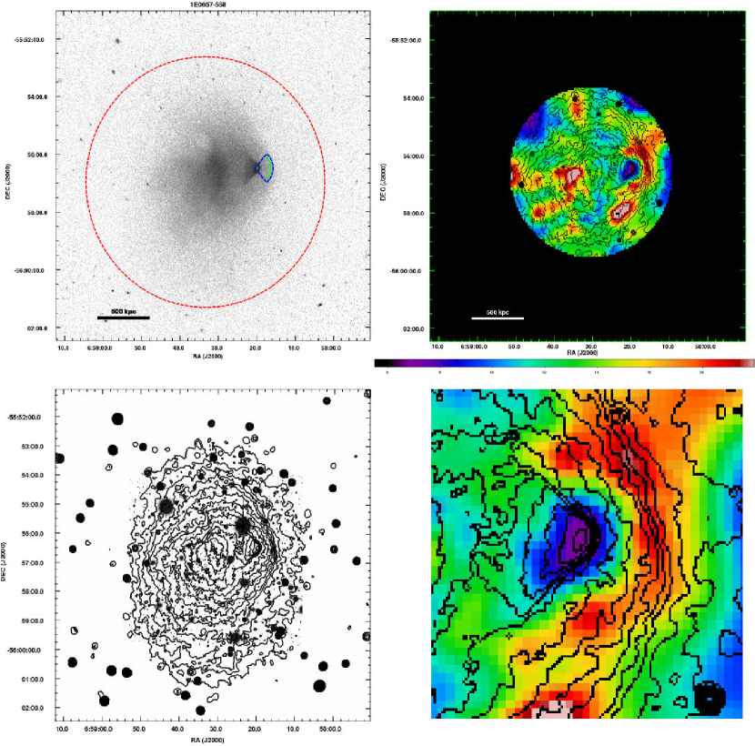
Figure 2.— Top left: background subtracted, exposure corrected, 0.5 – 7 keV Chandra  image of 1ES0657-558. The red region shows the area used to measure the global temperature in Section 2.3.1, and the blue region is where the surface brightness profile was fitted. The green arcs show the radial limits used for measuring the temperature inside and outside the cold front (the cold front delineates the two regions). North is towards the top of the page, and East is to the left. Top right: this image shows the projected temperature map produced as described in Section 3. The color scale is tuned so that different colors correspond to regions where temperatures differ by approximately $1\sigma$. Bottom left: Magellan IMACS $r$-band image (courtesy of D. Clowe). Bottom right: zoomed in version of the temperature map showing the region containing the cold front. The top right, bottom left and bottom right images have X-ray surface brightness contours overlaid.

The top right panel of Figure 2 shows the temperature map with surface brightness contours overlaid. The temperature structure is complex showing pockets of hot ($\sim 20$ keV) gas mixed with cooler ($\sim 12$ keV) gas. The only regular structure lies in the region containing the cold and shock fronts, where it can be seen that the subcluster/cold front coincides with the region of $\sim 7$ keV gas (slightly hotter than the temperature measured above of $\sim 5.8$ keV due to projection effects), significantly cooler than the surrounding gas, whilst the shock front coincides with an arc of $18-20$ keV gas. The hot regions on the eastern side of the main cluster are probably shock heated regions of either stripped subcluster gas, or main cluster gas. Previous temperature maps (Markevitch et al., 2002; Govoni et al., 2004) also show 1ES0657-558 to have a complex morphology with shock heated gas of up to 20 keV, consistent with the map presented here. However, the temperature map we present here has higher resolution and statistical quality, since it is derived from almost an order of magnitude more Chandra  data. Million & Allen (2008) used the same data set to produce a temperature map using an adaptive binning technique. The temperature map presented here agrees well with the Million & Allen temperature map.

The cluster hosts a luminous radio halo (Liang et al., 2000), and Govoni et al. (2004) showed that the halo brightness peaks correspond to hot spots in their temperature map, and the halo extends along the shock front. 1ES0657-558 has been the subject of a thorough campaign to map its mass distribution using the combination of weak and strong lensing (Clowe et al., 2006; Bradač et al., 2006), the results of which have shown an offset between the lensing mass distributions and the X-ray centroids providing compelling evidence for the existence of dark matter (Clowe et al., 2006). These results, combined with the observations of Barrena et al. (2002) and Markevitch et al. (2002) show that the subcluster is probably caught just after its first (slightly off center) core passage, traveling from the south-east, and the merger occurs mostly in the plane of the sky, with the velocity difference between the main cluster and the subcluster only $\sim 600$$\,\rm{km\,s^{-1}}$(Barrena et al., 2002). The velocity of the shock derived by Markevitch & Vikhlinin (2007) is 4700$\,\rm{km\,s^{-1}}$, although in reality the subcluster is unlikely to be traveling at such a high velocity (see, for example, Springel & Farrar, 2007; Milosavljević et al., 2007).

4.1.2 Abell 3667

Abell 3667 was one of the original cold front clusters observed with Chandra  and, along with Abell 2142, provided the defining characteristics of cold fronts (Vikhlinin et al., 2001a). Abell 3667 has an X-ray luminosity of $L_{\rm X}(0.4-2.4\,{\rm keV})=5.1\times 10^{44}\,{\rm erg\ s^{-1}}$ (Ebeling et al., 1996), temperature $kT\sim 7$ keV (Knopp et al., 1996; Markevitch et al., 1998; Vikhlinin et al., 2001a; Briel et al., 2004), Abell richness class 2 and a redshift of z=0.055. In the top left panel of Figure 3 the Chandra  X-ray image of the central core region of Abell 3667 is presented revealing a complex morphology which is elongated along a south-east to north-west direction with the cold front being the most prominent feature to the south-east. The front appears regular at small opening angles, but fans out at larger angles to form a mushroom-cap-like shape. The same morphology is also prominent in the temperature map in the top right panel of Figure 3 which shows clearly that the front delineates regions of cool ($\sim 4.5$ keV) gas from the ambient ICM with temperature ($\sim 7$ keV). As noted by Briel et al. (2004), the gas at the tip of the front is coolest ($\sim 4$ keV). Heinz et al. (2003) use simulations to show motions inside a remnant gas core are induced due to the flow of gas around the cloud. These internal motions move lower entropy gas towards the tip of the cold front and, as the gas moves to the tip of the cold front, it cools due to adiabatic expansion, enhancing the temperature contrast at the tip of the front. The temperature map presented here is in good agreement with those presented in the literature (Markevitch et al., 1999; Vikhlinin et al., 2001a; Mazzotta et al., 2002; Briel et al., 2004), although the longer combined exposure time of the Chandra  data presented here gives a more statistically significant map with higher spatial resolution. The map shows a complex morphology of hot and cool gas patches, including a patch of significantly hotter ($\sim 9-10$ keV) gas to the north-west of the cluster center.

At the cold front, a density jump of $2.6\pm 0.2$ is measured (see Table 3). This value is inconsistent with the value of $3.9\pm 0.8$ measured by Vikhlinin et al. (2001a). This is because Vikhlinin et al.’s density measurement just outside the front is obtained by extrapolating their $\beta$-model electron density model from larger radii to the front position. Their aim was to determine the pressure in the undisturbed region of the flow around the front, so they tried to correct for gas within the “compression” region just outside the front where they note that the surface brightness $\sim 70$ kpc exterior to the front exceeds that predicted by their $\beta$-model. For the density measurement made here, the power law density model describing the surface brightness outside the front is approximately limited to this $\sim 70$ kpc region, meaning a higher density just outside the front is measured compared to that of Vikhlinin et al., which leads to a lower density jump.

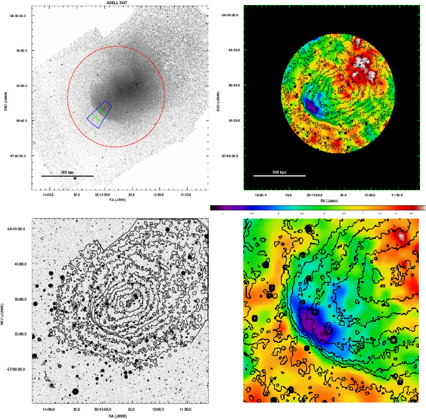
Figure 3.— Same as Figure 2 but for Abell 3667 and with a Supercosmos Sky Survey $r_{\rm F}$-band image at the lower left.

Abell 3667 presents clear evidence for merger activity at both optical and radio wavelengths. Observations at radio wavelengths show Abell 3667 is one of a handful of objects which harbor two diffuse radio relic sources (Rottgering et al., 1997)—one to the north-west and one to the south-east. The radio observations also show two tailed radio galaxies, one of which lies on an axis joining the two dominant cluster galaxies with its tail pointing along this axis (Rottgering et al., 1997). Radio relics are thought to trace merger shock fronts and Roettiger et al. (1999) were able to reproduce the basic radio morphology of the relics using magnetohydrodynamic/N-body simulations of a slightly off-center merger with a 5-to-1 mass ratio and the subcluster impacting from the south-east to the north-west, being observed $\sim 1$ Gyr after core passage. The simulations also reproduced the basic observed X-ray morphology and galaxy distribution.

Optical observations have shown the galaxy density distribution is bimodal, with the second density enhancement centered on the second brightest cluster galaxy (Proust et al., 1988; Sodre et al., 1992; Owers et al., 2009a). Significant emission associated with the secondary density enhancement was detected in the ROSAT X-ray observations of Knopp et al. (1996), lying just out of the field of view of the Chandra  observations. Using weak lensing, Joffre et al. (2000) found evidence for substructure in their mass maps which coincides with this secondary density enhancement. Sodre et al. (1992) found the second D galaxy has a velocity offset of $\sim 400$$\,\rm{km\,s^{-1}}$  compared the the central D galaxy, and the velocity distribution surrounding this second D galaxy appears to indicate that it forms a dynamical subunit within the cluster.

Abell 3667 was the subject of comprehensive optical follow-up with the aim of showing the cold front was related to merger activity in Owers et al. (2009a). Using combined spatial and velocity information for a large sample of spectroscopically confirmed cluster members, Owers et al. found the cluster can be separated into two major components, coinciding with the density enhancements found by Sodre et al. (1992) and separated in peculiar velocity by $\sim 500$$\,\rm{km\,s^{-1}}$, plus a number of smaller subgroups. These observations indicate Abell 3667 is undergoing a major merger which has produced the observed cold front.

4.1.3 Abell 1201

Abell 1201 is one of the least well studied clusters in the sample and has an Abell richness class 2 (Abell et al., 1989), redshift z=0.168 (Struble & Rood, 1999) with an X-ray luminosity $L_{\rm X}(0.1-2.4\,{\rm keV})=2.4~{}\times~{}10^{44}\,\rm{ergs}\,\rm{s}^{-1}$ (Böhringer et al., 2000). The top left panel of Figure 4 shows the Chandra  image of Abell 1201 which is elongated along a south-east to north-west axis, with the main cold front clearly visible to the south-east, a bright central core which also has a cold front towards the north-west and a remnant core also visible to the north-west. The temperature map shown in the top right panel of Figure 4 reveals a hot $\sim 7$ keV region lying between the main cluster core and the remnant core, indicating some form of heating here probably caused by adiabatic compression due to core motion. There is no evidence for significant temperature differences at the location of the remnant core (c.f. 1ES0657-558 where the remnant core clearly stands out in the temperature map). This may be attributed to the heavy smoothing required to obtain well-defined temperatures, since this observation was significantly affected by strong flares, so that nearly half of the exposure was rejected during cleaning. There is a cool ($\sim 4$ keV) stream of gas connecting the cold front to the cool core of the main cluster in the temperature map. This indicates that the cold gas associated with the front is gas which has been displaced from the cool core of the cluster, and the front is probably associated with a spiral-like structure (for example as seen in the temperature maps for MS1455.0+2232 and RXJ1720.1+2638 in the top right panels of Figures 9 and 8, respectively) seen in projection, similar to those seen in the $x$ projection image presented in Figure 19 of Ascasibar & Markevitch (2006).

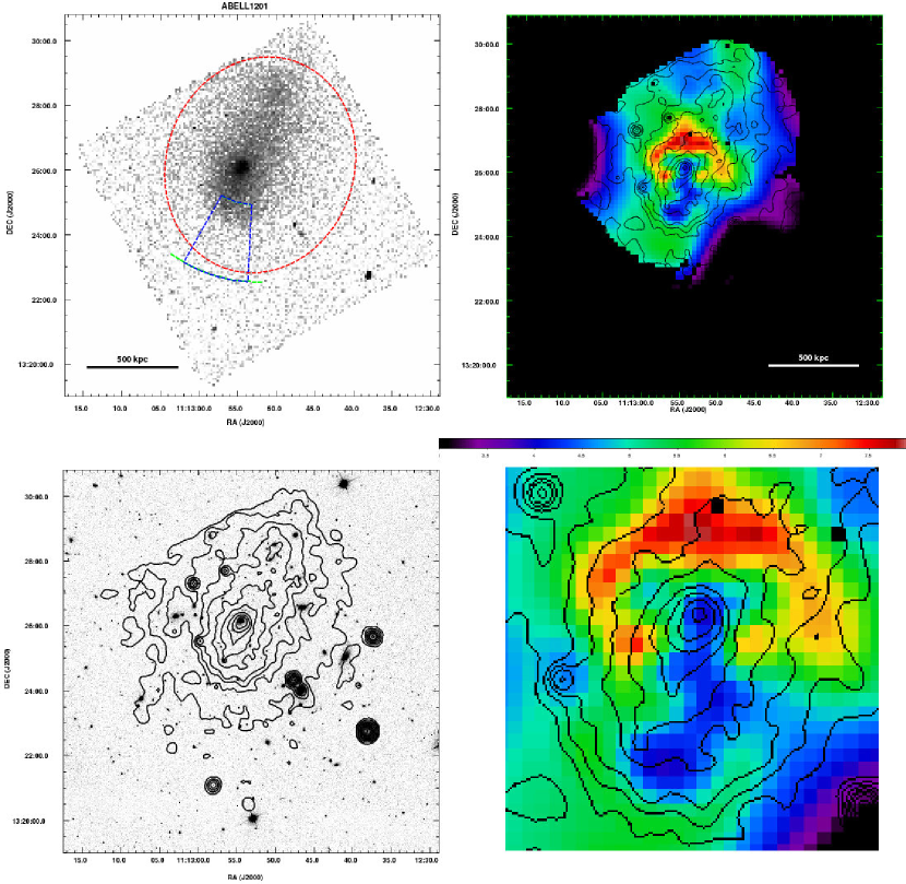
Figure 4.— Same as Figure 2 but for Abell 1201 and with an SDSS $r$-band image at the lower left.

Detailed follow up multi-object optical spectroscopy of Abell 1201 has been undertaken and is presented in Owers et al. (2009b). This study shows a bimodal galaxy density distribution with the main component centered on the main X-ray core and a second component coincident with the remnant core to the north-west. The combination of spatial and velocity information also reveals the presence of substructure coincident with the remnant core and offset in peculiar velocity by $\sim 430$$\,\rm{km\,s^{-1}}$, indicating a merger is occurring with the majority of its velocity in the plane of the sky. The perturbation from this merger has given rise to the cold fronts caused by sloshing of the ICM.

Edge et al. (2003) discovered a small scale gravitational arc in Abell 1201, and proposed the observed arc properties could be explained by a mass distribution which was either highly elliptical or bimodal. The data allowed a bimodal model with a secondary mass clump lying to the south-east of the cluster center, however, Edge et al. favored the model with high ellipticity. Given the results of Owers et al. (2009b), it would seem that a bimodal mass distribution is the most likely explanation for the data, although the center of mass of the second component is coincident with the north-west remnant core.

4.1.4 Abell 2069

Abell 2069 is a richness class 2 (Abell et al., 1989) cluster at redshift z=0.116, which was originally shown to have multiple condensations in the gas and galaxy distributions by Gioia et al. (1982) and is part of a large supercluster containing some 6 clusters (Einasto et al., 1997). The top left panel of Figure 5 shows the Chandra  image of Abell 2069 (binned to $7.8^{\prime\prime}$ pixels) which shows the main component (Abell 2069A in the terminology of Gioia et al., 1982) to be elongated along a south-east to north-west axis. There are two bright elliptical galaxies aligned along this axis which differ in peculiar velocity by only $\sim 230$$\,\rm{km\,s^{-1}}$ (Gioia et al., 1982). Abell 2069B can be seen to the north-east and it hosts a cold front towards the north-west along with a fan like extension of X-ray emission towards the south-east. There is a dominant elliptical galaxy associated with Abell 2069B which has a redshift z=0.1178 and is surrounded by an overdensity in the projected galaxy number surface density (Gioia et al., 1982). Assuming the redshift of the dominant elliptical is representative of Abell 2069B, then its peculiar velocity with respect to the mean cluster redshift is only $485$ $\,\rm{km\,s^{-1}}$. Although the cold front is associated with the Abell 2069B, it is difficult to determine whether the nature of this cold front is consistent with a contact discontinuity occurring at the interface of the lower entropy Abell 2069B ICM and the higher entropy Abell 2069A ICM, or a cold front induced by sloshing of the Abell 2069B gas. Given the small peculiar velocity offset of Abell 2069B and Abell 2069A, it can be concluded that the majority of the subcluster motion is in the plane of the sky.

The resolution of the temperature map presented in the top right panel of Figure 5 is limited by a lack of photons. However, it does show that the projected temperature around Abell 2069B is significantly cooler than the ICM surrounding it, and also that Abell 2069A hosts a complex temperature distribution with regions of $6-8$ keV gas interspersed with pockets of cooler $\sim 4$ keV gas. The temperature structure in Abell 2069A may be due to a core crossing by Abell 2069B. In particular the region of $6-8$ keV gas to the east may be due to the north-east bound passage of Abell 2069B. In this case, the cold front in Abell 2069B is more likely to be due to sloshing of the Abell 2069B gas. However, the existence of the two dominant elliptical galaxies may be indicative of merger activity within Abell 2069A itself and this could also explain the complex temperature structure.

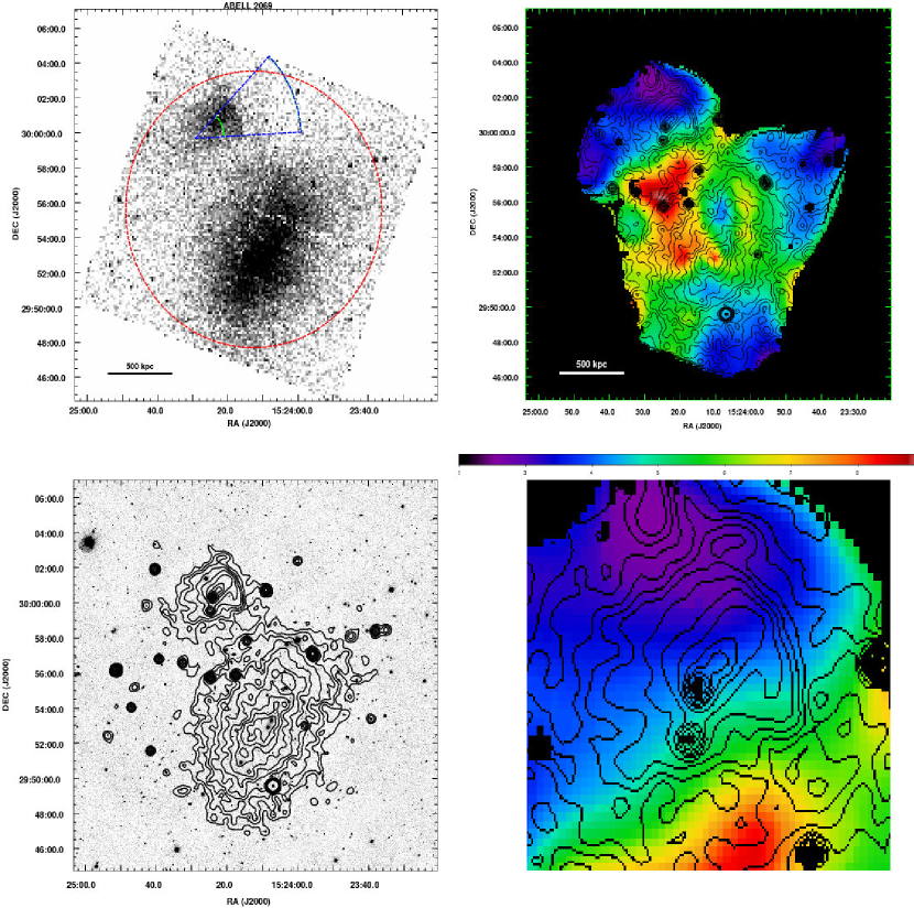
Figure 5.— Same as Figure 2 but for Abell 2069 and with an SDSS $r$-band image at the lower left.

4.1.5 Abell 1758N

Abell 1758 is a rich (Abell richness class 3; Abell et al., 1989) double cluster at redshift z=0.279 (Struble & Rood, 1999). The Chandra  observations, which were originally presented in David & Kempner (2004), were taken on the ACIS-S3 chip and contain only the northern component of the double cluster which is referred to as Abell 1758N. The David & Kempner (2004) study showed the X-ray morphology is irregular with two main components placed on an axis running from the south-east to the north-west. The David & Kempner (2004) study also showed that the morphology of the north-west component is fan-like with a tail of gas extending to the south, and a cold front located towards the north, suggesting the motion of the substructure is towards the north. These features can be seen in top left panel of Figure 6 where Chandra X-ray image is reproduced. Using a truncated spheroid to model the surface brightness across the front, David & Kempner (2004) measured a density jump of $1.6\pm 0.2$ ($1\sigma$ errors) which is consistent within the errors with the value presented in Table 3. The north-west and south-east structures are coincident with peaks in the projected galaxy number density maps presented in Dahle et al. (2002) and also with substructure in the lensing maps of Okabe & Umetsu (2008). There is a second less significant front further south-east of the south-east structure for which David & Kempner (2004) measured a density jump of $\sim 1.5\pm 0.2$. They used a hardness ratio map to show that the gas inside the front is cooler than outside, thus concluding it is also a cold front caused by the interface of low entropy subcluster gas with the higher entropy ambient ICM. Coincident with the parcel of low entropy gas responsible for the south-east cold front is another overdensity of galaxies housing a bright elliptical galaxy.

The top right panel of Figure 6 shows the temperature map for Abell 1758N, which only covers a small area due to the low number of photons detected, particularly in the outskirts. The map shows the two components host significantly cooler gas compared to the hotter gas in the outskirts. The absence of a sharp temperature jump at the cold front is mainly due to the poor effective resolution of the temperature map. This means the cold front regions are contaminated by the hotter gas from the outskirts, thus the temperature measured here is the average of the two contributions. There is a bridge of cool gas joining the two subclusters, and a tongue of cool gas trailing the south-east subcluster which is presumably ram pressure stripped gas due to the collision of these two subclusters. The features seen in the temperature map are qualitatively similar to those seen in the hardness ratio map of David & Kempner (2004).

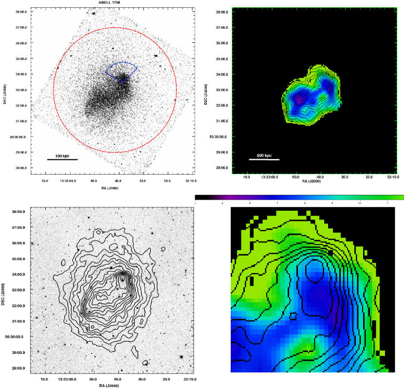
Figure 6.— Same as Figure 2 but for Abell 1758 and with an SDSS $r$-band image at the lower left.

Based on the X-ray characteristics, David & Kempner (2004) presented a merger scenario for Abell 1758N whereby the system is being viewed after a recent off-axis pericentric passage of two $\sim 7$ keV clusters, and the significantly hotter gas in the outskirts has been heated by merger shocks. Indirect evidence for merger activity occurs at radio wavelengths where, at the position of the south-east cold front, there is a narrow-angle tailed (NAT) radio galaxy which has its tail extending from the north-west to the south-east (O’dea & Owen, 1985), and its head coincident with a fainter galaxy to the north-east of the dominant south-east elliptical. Bliton et al. (1998) showed that NAT galaxies are preferentially found in clusters with substructure, concluding that at least part of the relative velocities required to produce a NAT is due to bulk gas motions generated during a merger. Further Chandra  observations with longer exposures would enable the measurement of pressure differentials at the cold front, thus constraining gas velocities and allowing the components of the relative velocities of the gas and NAT galaxy to be constrained.

Given the fan-like morphology and its coincidence with a galaxy overdensity, it appears the north-west cold front in Abell 1758N is a merger induced cold front generated at the interface of colliding subclusters.

4.1.6 Abell 2163

Abell 2163 is one of the hottest (kT = 15.5 keV; Maughan et al., 2008), most luminous ($L_{\rm X}[0.1-2.4\,{\rm keV}]=22.9\times 10^{44}\,{\rm erg\ s^{-1}}$; Ebeling et al. 1996) clusters of galaxies known. It has a redshift of $z=0.201$, Abell richness class 2 (Abell et al., 1989) and has been the subject of many studies at multiple wavelengths (e.g.; Maurogordato et al., 2008; Feretti et al., 2004; Markevitch & Vikhlinin, 2001; Feretti et al., 2001; Squires et al., 1997; Holzapfel et al., 1997). The Markevitch & Vikhlinin (2001) Chandra observations of Abell 2163 revealed a cluster with an irregular morphology with an extension along a direction going north-east to south-west, as seen in deeper Chandra image presented in top left panel of Figure 7. There is a cold front in the south-west which appears to have a mildly convex shape and is not as sharp as others seen in this sample (e.g. the cold front seen in Abell 3667), possibly indicating the front has significant inclination with respect to the plane of the sky or is in the process of breaking up. There is a group due north and a hint of excess emission east of the core emission. The temperature map shown in the top right panel of Figure 7 shows the cluster exhibits a complex multi-temperature gas distribution with the cold front associated with $\sim 8$ keV gas and surrounded by hotter $\sim 11$ keV gas, consistent with the temperature jump given in Table 3 within the errors. The regions corresponding to the X-ray extension towards the south-east and the excess X-ray emission to the east are significantly hotter than the rest of the cluster at $>14$ keV. The infalling group to the north is significantly cooler than the main cluster at 5-6 keV according to the temperature map. The temperature map presented here is in good agreement with the maps published by Govoni et al. (2004) and Markevitch et al. (2001), although we obtain higher resolution and statistical quality by simultaneously fitting the two Chandra data sets to produce the temperature map.

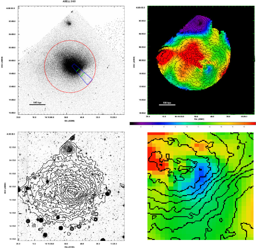
Figure 7.— Same as Figure 2 but for Abell 2163 and with a CFHT $r$-band MegaCam image at the lower left.

As mentioned above, Abell 2163 has been studied extensively at multiple wavelengths and evidence for merger activity presents itself in the majority of these observations. The first indications that Abell 2163 was an atypical cluster came from combined Ginga and Einstein X-ray observations which showed an extremely high temperature (Arnaud et al., 1992). Further ROSAT and ASCA observations confirmed the high temperature and also showed evidence for temperature and surface brightness structure in the ICM, suggesting evidence for merger activity (Markevitch et al., 1994; Elbaz et al., 1995; Markevitch, 1996). High resolution Chandra  temperature maps presented in Markevitch et al. (2001) and Govoni et al. (2004) revealed this temperature structure in greater detail, showing in particular that the central region harbors complex temperature structure which is consistent with a major merger, along with the group towards the north seen in the ROSAT images. Squires et al. (1997) shed light on the dynamical state of the cluster showing the distributions of both mass and galaxies are bimodal in the center, with the peaks in each distribution roughly coincident, and concluded the cluster is not in a relaxed dynamical state. At radio wavelengths, Abell 2163 hosts a luminous radio halo, a possible radio relic, along with 3 tailed radio galaxies all with tails oriented in the same direction towards the west (Feretti et al., 2001). Finally, Maurogordato et al. (2008) present an analysis of the cluster dynamics from a sample of 361 cluster member redshifts which show a multi-modal velocity distribution, strong velocity gradients along a north-east to south-west axis along with multiple clumps in the galaxy surface density. These results were confirmed by Owers (2008) where the analysis of a sample of 491 cluster member redshifts showed a significantly skewed velocity distribution and significant dynamical substructure when spatial and velocity information was combined. In particular, substructure was found to coincide with the cold front seen in Figure 7, strongly supporting the argument that this cold front is caused by an ongoing cluster merger.

4.2. Clusters with relaxed Appearing X-ray Morphologies

4.2.1 RXJ1720.1+2638

RXJ1720.1+2638 was the first of the otherwise relaxed appearing clusters which were revealed to have cold fronts by Chandra  (Mazzotta et al., 2001). It has an X-ray luminosity of $L_{\rm X}(0.1-2.4\,{\rm keV})=7.3\times 10^{44}\rm erg\ s^{-1}$ (Böhringer et al., 2000) and redshift $z=0.1605$ (Owers, 2008). The top left panel of Figure 8 shows the Chandra  X-ray image of RXJ1720.1+2638 which reveals a relaxed overall morphology with a bright core and a cold front towards the south-east. Mazzotta & Giacintucci (2008) also report a cold front towards the north-west of the core which has a density jump of $\sim 1.68$. It is noted that Mazzotta & Giacintucci (2008) measured a density jump of $1.66\pm 0.05$ for the south-east cold front, inconsistent with the value given in Table 3. This is because Mazzotta & Giacintucci (2008) measured the density jump over a larger opening angle, which included regions where the front is less well defined. The temperature map presented in the top right panel of Figure 8 reveals more about the nature of the cold front. There is a finger of cool gas starting at the surface brightness peak and spiraling in an anticlockwise direction before terminating at the cold front, also seen in the temperature maps of Mazzotta & Giacintucci (2008), and similar to the temperature structure seen in the simulations of Ascasibar & Markevitch (2006, see their Figure 7). On larger scales the temperature map is patchy with regions of hot $\sim 8$ keV gas surrounded by ambient $\sim 6$ keV gas.

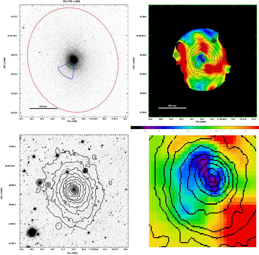
Figure 8.— Same as Figure 2 but for RXJ1720.1+2638 and with an SDSS $r$-band image at the lower left.

Dahle et al. (2002) report on the distribution of galaxies, light and dark matter within RXJ1720.1+2638, finding the light distribution to be fairly regular and dominated by the central cluster galaxy. The weak lensing mass distribution appears to be less regular, with the main signal roughly coincident with the cluster center and a secondary peak detected $\sim 2-3$ arcmin to the south-west. The galaxy number density also appears to be fairly regular, although there is an extension of the contours towards the south-west in the direction of the secondary mass clump detected in the weak lensing maps. RXJ1720.1+2638 is by all accounts a fairly relaxed looking system, and, along with MS1455.0+2232, is thus a very important test case within our sample, given the hypothesis that cold fronts are a result of major merger activity. For this reason, RXJ1720.1+2638 was selected for follow up observations using multi-object spectroscopy. The results of the study are presented in Owers (2008) and show evidence for substructure in the galaxy density distribution and also when spatial and velocity information is combined. However, the substructure’s relation to the cold front remains ambiguous, and further observations are required.

4.2.2 MS1455.0+2232

MS1455.0+2232 (also known as ZW7146) was discovered serendipitously as an extended X-ray source in the Einstein Observatory Extended Medium–Sensitivity Survey (EMSS; Gioia et al., 1990) and later reported to host a massive 1500$\rm{M}_{\odot}$$yr^{-1}$ cooling flow (Allen et al., 1996). The top left panel of Figure 9 shows the Chandra  X-ray image of MS1455.0+2232 which has a relaxed X-ray morphology, harboring a slight ellipticity with major axis running from the south-west to north-east with a mild asymmetry along this axis. Also along this axis is the cold front as outlined by the blue annular segment in the top left panel of Figure 9. Inspection of the temperature map presented in the top right panel of Figure 9 reveals a spiral-like feature of cool gas beginning at the cool core and ending at the position of the cold front. This feature is also seen in the temperature map of Mazzotta & Giacintucci (2008), which is derived from the same Chandra data set, and shows good overall agreement with the map presented here. The cold front appears similar to those seen in the simulations of Ascasibar & Markevitch (2006) (see Figure 7 and Figure 19) where an off-center merger of a gasless dark matter halo disturbs the cool cluster core, offsetting both the gas and dark matter from its initial position. The offset low entropy gas does not fall back into the core along a purely radial path, since it has acquired angular momentum from the infalling dark matter halo, and thus a spiral pattern is formed.

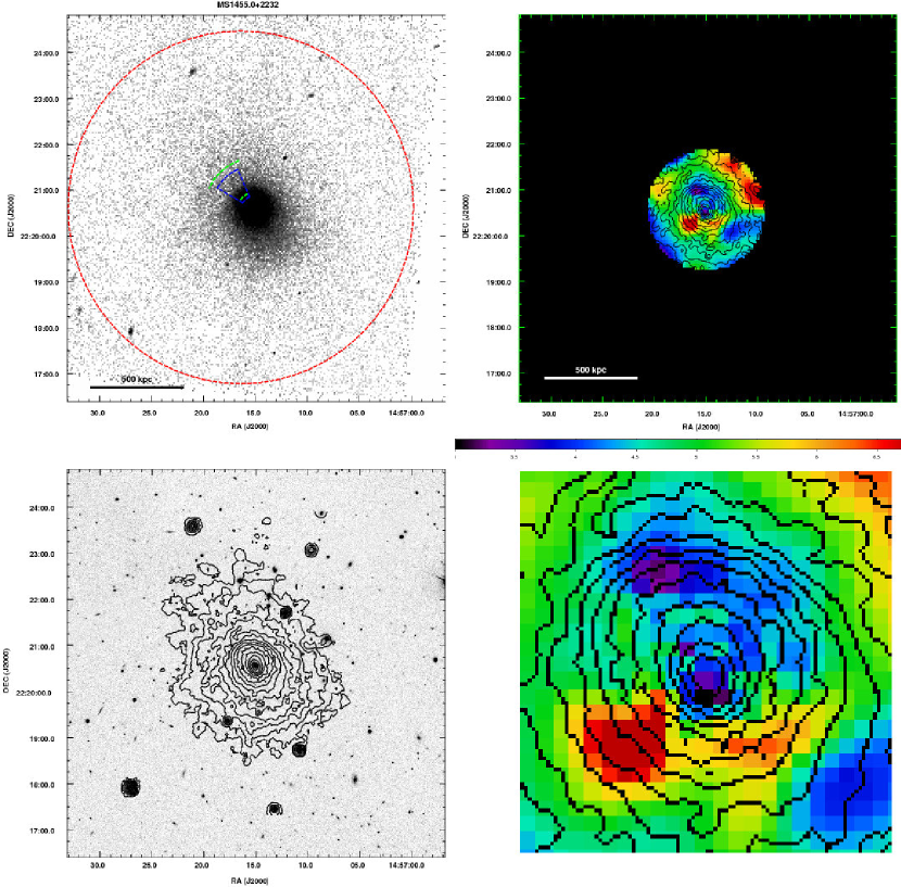
Figure 9.— Same as Figure 2 but for MS1455.0+2232 and with an SDSS $r$-band image at the lower left.

Further evidence for merger activity in MS1455.0+2232 comes from the weak lensing maps of Dahle et al. (2002), where, despite showing a fairly regular projected galaxy number density distribution, the weak lensing maps showed a highly elliptical morphology with major axis pointing along an axis going from south-west to north-east (similar to the X-ray major axis angle). Smail et al. (1995) found the position angle for the mass, gas and projected galaxy density distributions within $\sim 1.25$ arcmin ($\sim 300$ kpc) are all aligned along the same axis. The combined radio and X-ray observations of Mazzotta & Giacintucci (2008) have shown a spatial correlation between the spiral structure and radio emission associated with a core mini radio halo, suggesting a population of relic electrons injected by the central AGN have been reaccelerated by turbulence associated with the gas motions causing the cold fronts.

4.2.3 Abell 2142

The first cold fronts were discovered in Chandra  observations of Abell 2142 (Markevitch et al., 2000). The cluster is optically rich (Abell richness class 2; Abell et al., 1989), hot (kT=9 keV; White et al., 1994; Allen & Fabian, 1998; Markevitch et al., 1998, 2000), X-ray luminous ($L_{\rm X}[0.1-2.4\,{\rm keV}]=11.4\times 10^{44}\rm erg\ s^{-1}$; Böhringer et al. 2000) with redshift z=0.089 and velocity dispersion $\sigma=1280$$\,\rm{km\,s^{-1}}$  (Oegerle et al., 1995). The top left panel of Figure 10 shows the Chandra  X-ray image of Abell 2142 which has an elliptical morphology with its position angle aligned along a south-east to north-west axis. Along this axis and to the north-west is the cold front for which density and temperature jumps were measured, whilst a second less prominent cold front, noted by Markevitch et al. (2000), lies just south of the core. The north-west cold front appears to have a cometary morphology with the sharp brightness edge to the north-west forming the head, and a tail pointing towards the south-east where the surface brightness drops less sharply with radius. The temperature map presented in the top right panel of Figure 10 is generated using a much longer exposure (ObsID 5005 data) than the one shown in Markevitch et al. (2000) and reveals a complex temperature distribution, where the two cold fronts clearly separate regions of cool and hot gas. The temperature morphology of the central region is very similar to that seen by Markevitch et al. (2000), i.e., the brightness peak is much cooler ($\sim 6$ keV) than the gas at larger radii, and there is a finger of $\sim 7$ keV gas extending from the core towards the north-west. The regions inside the north-west cold front are hotter than the core gas, at $\sim 8-9$ keV, but significantly cooler than the gas at larger radii outside the front ($>12$ keV). Note that towards the south-east, the gas temperature is around $7-8$ keV, inconsistent with the rise in temperature seen in the same region by Markevitch et al. (2000). This difference is likely attributed to the different data sets used—Markevitch et al. (2000) used early ACIS-S data where the calibration was poorly known, whereas here the ACIS-I data are used along with the latest and much improved calibration files.

The exact nature of the cold fronts is uncertain. Markevitch et al. (2000) propose they are due to the survival of dense subcluster cores during a major merger, but later Markevitch & Vikhlinin (2007) claim the cold fronts are more likely to be the result of core gas motion (not unlike RXJ1720.1+2638, MS1455.0+2232 and Abell 1201 of this sample). However, Abell 2142 seems anomalous since, while there is a finger of cool gas extending from the core towards the north-west, this finger does not form a coherent spiral-like temperature structure joining the core to the north-western cold front, as seen in the clusters MS1455.0+2232 and RXJ1720.1+2638. This of course could be due simply to different viewing angles, since the existence of multiple fronts lying on different sides of the cluster core is fairly compelling evidence for sloshing type cold fronts.

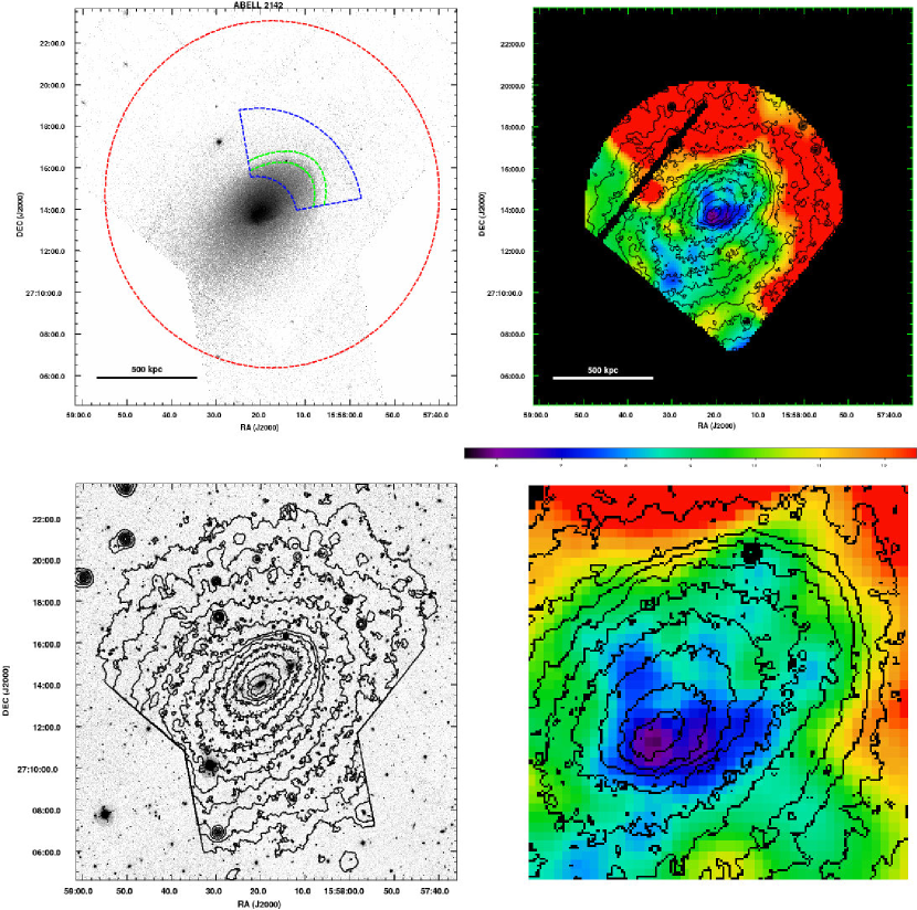
Figure 10.— Same as Figure 2 but for Abell 2142 and with an SDSS $r$-band image at the lower left.

Power ratio analyses of ROSAT X-ray images gave an indication that Abell 2142 was a dynamically active system (Buote & Tsai, 1996), and the case for a merger was strengthened by the analysis of Henry & Briel (1996), which showed strong variations in the azimuthal temperature distribution. In an earlier study using 103 cluster member redshifts, Oegerle et al. (1995) found evidence for substructure at the $90\%$ confidence level using the Dressler-Shectmann $\Delta$ test, although they were unable to isolate the substructure spatially or in velocity space and conclude Abell 2142 is a cluster with uncertain dynamics. Indirect evidence for dynamical activity came from the observation of two dominant bright elliptical galaxies in the cluster core, with one having a redshift consistent with the cluster mean redshift and the second offset in peculiar velocity by $\sim 1600$$\,\rm{km\,s^{-1}}$. Further evidence for dynamical activity came from the weak lensing maps of Okabe & Umetsu (2008), who found evidence for a significant excess in their weak lensing signal at a projected distance of $\sim 540$ kpc ahead of the north-west cold front. At radio wavelengths, Abell 2142 exhibits diffuse radio emission extending $\sim 350$k̇pc about the cluster core, although it is unclear whether this is part of a massive radio halo associated with a cluster merger (Giovannini et al., 1999). Bliton et al. (1998) show a NAT source which has a tail extending away from the cluster center and in roughly the same direction as the major axis of the X-ray emission. This NAT galaxy is displaced by $\sim 1400$$\,\rm{km\,s^{-1}}$  from the cluster rest frame, and its head is located just within the edge of the north-west cold front (coincident with the X-ray point source seen to lie just within the north-west cold front in Figure 10). Despite the uncertain nature of the merger geometry, it is clear that Abell 2142 is a dynamically active cluster.

5. Discussion

Selecting clusters based purely on the existence of a cold front has produced a sample with two distinct X-ray morphological types: those with clearly disturbed X-ray morphologies (Section 4.1) and those with fairly relaxed X-ray appearances, aside from the cold fronts (Section 4.2). In Table A High Fidelity Sample of Cold Front Clusters from the CHANDRA Archive, the evidence indicating merger activity for the cold front sample, along with the X-ray morphologies, is summarized. Once again, to emphasize the dichotomy, the clusters in Table A High Fidelity Sample of Cold Front Clusters from the CHANDRA Archive are separated into the two subsamples presented in Section 4.

Of the six clusters in Section 4.1, five have significant evidence for merger-related activity at other wavelengths and, as was evident from their X-ray morphologies, it is clear the existence of a cold front is good evidence for merger activity. The sixth cluster, Abell 2069, does have evidence for substructure in its projected galaxy density Gioia et al. (1982), although it is not as well studied at multiple wavelengths when compared to the other five clusters, thus the evidence for merger-related activity at other wavelengths is less compelling. Within this subsample there are a broad range of X-ray morphologies. This can be traced to the different formation mechanisms for cold fronts which depend on the details of the merger event (e.g. merger stage, mass of subcluster, impact parameter or the existence of cool cores; Poole et al., 2006). For example, upon comparing Abell 1201 to 1ES0657-558, it can be seen that both contain remnant cores observed after pericentric passage. However, Abell 1201’s cold front is due to gas sloshing of the primary’s cool core, while the cold front in 1ES0657-558 occurs in the remnant core and there is no evidence for a cold front due to motion of its primary’s core. Two scenarios relating the details of the initial conditions of the mergers to the cold front formation can explain this: (1) The primary in 1ES0657-558 did not contain a significant cool core, thus no cold fronts analogous to those in Abell 1201 are seen. (2) The impact parameters of the mergers differ significantly, i.e., the merger in the 1ES0657-558 was almost directly head on, thus the primary’s core was destroyed by the secondary’s passage, while the pericentric passage of the secondary in Abell 1201 was off-axis and did not significantly disrupt the cool core allowing the formation of the cold fronts. Thus, aside from being good merger signposts, cold fronts also provide additional information which can be used in tandem with observations at other wavelengths to constrain the merger histories in these clusters.

Turning to the clusters in Section 4.2, Table A High Fidelity Sample of Cold Front Clusters from the CHANDRA Archive shows that currently there is very little observational evidence in the literature to determine a clear cut explanation for the cold fronts in clusters with overall relaxed morphologies. The simulations of Ascasibar & Markevitch (2006) showed that pure gravitational disturbances in the form of infalling gasless dark matter subclumps are able to produce these cold fronts whilst maintaining the overall relaxed appearance. Commonly seen in simulations of this scenario are spiral-like temperature structures, which we also see in the temperature maps of RXJ1720.1+2638 and MS1455.0+2232 (Figures 8 and 9, respectively), showing the cool gas causing the front to be connected to the cool cluster core. Also apparent in these simulations are the existence of multiple cold fronts at different radii; a signature clearly observed in Abell 2142. Marginal evidence is found favoring this scenario in RXJ1720.1+2638  (Owers, 2008), where there is substructure in the galaxy density distribution but no apparent secondary structure in the X-ray image. With further optical data, RXJ1720.1+2638, Abell 2142 and MS1455.0+2232 could provide definitive tests of the scenario put forth by Ascasibar & Markevitch (2006) where an essentially gas-free group perturbs the core ICM, setting off sloshing whilst providing minimal further evidence of a merger at X-ray wavelengths.

While much of the evidence favoring a merger origin for the relaxed appearing sloshing type cold front clusters comes from simulations, two significant observations exist which show the plausibility of merger-induced sloshing as a mechanism for the formation of cold fronts. The XMM observations of Abell 1644 (Reiprich et al., 2004; Markevitch & Vikhlinin, 2007) and the Chandra  observations of Abell 1201 presented here and in Owers et al. (2009b) both reveal sloshing cold fronts and also remnant cores which are apparently causing the perturbation. The optical follow up observations of Abell 1201 showed evidence for localized velocity substructure coincident with the remnant core (Owers et al., 2009b), confirming it is a significant merging substructure, although the latest optical observations of Abell 1644 do not reveal significant evidence for localized velocity substructure (Tustin et al., 2001). Without detailed simulations of these two particular objects, it is unclear whether they will evolve into relaxed appearing clusters with cold fronts, like those presented in Section 4.2. Nevertheless, it is clear that both Abell 1644 and Abell 1201 provide strong empirical evidence of merger-induced sloshing as a viable mechanism for producing cold fronts.

Perhaps the most appealing outcome that studies of cold front clusters offer is the possibility of using them to distinguish major and minor mergers. Clearly the clusters in Section 4.1 are systems which are undergoing significant dynamical evolution and are most likely major mergers. However, the same conclusion cannot be drawn based on the evidence available for the clusters presented in Section 4.2. As discussed above, Ascasibar & Markevitch (2006) found that only a relatively minor merger was required to produce cold fronts in relaxed appearing clusters. Future dynamical analyses of RXJ1720.1+2638, Abell 2142 and MS1455.0+2232 at optical wavelengths will determine the level of dynamical activity required to produce a cold front. If it turns out to be true that the appearance of these clusters can be explained by minor mergers, then the combination of the existence of a cold front and X-ray morphology will provide a useful diagnostic for discriminating major and minor mergers in clusters.

6. Summary and Conclusions

We have presented and described in detail a sample of nine clusters selected from the Chandra archive based purely on the existence of cold fronts in their ICM. These clusters are the subject of an ongoing study to determine if cold fronts may be used to reliably identify recent cluster-cluster mergers.

In selecting the cold front sample, particular attention was paid to obtaining highly reliable identifications. To this end, each cluster met the following strict selection criteria: A total Chandra exposure time greater than 40ks, $0.05<z<0.3$, a visible surface brightness edge in the X-ray image which has a density jump exceeding 1.5 at the lower $90\%$ confidence level, the measured gas temperature must be lower on the denser side of the front, and the pressure must be continuous across the front within the errors. This resulted in the identification of nine cold front clusters for which we present temperature maps, X-ray and optical images and an overview of the multiwavelength evidence for merger activity available in the literature. The key conclusions of this study are as follows:

• the measurement of thermal properties across the fronts was an essential diagnostic tool; Abell 2034 and Abell 665 were rejected on this basis, since their fronts were better explained as shocks. These are very likely merger shocks and if these clusters were to remain in our sample, the contamination would not be harmful when considering the aim is to use cold fronts as reliable signposts of merger activity.

• There is a dichotomy within the sample of cold front clusters: those which harbor clearly disturbed X-ray morphologies, and those which appear to have fairly relaxed X-ray morphologies, apart from the existence of a cold front.

• The majority of those clusters with disturbed X-ray morphologies have significant evidence for merger activity at multiple wavelengths, while minimal evidence for a merger exists at other wavelengths in the relaxed appearing clusters.

• Two of the relaxed appearing clusters (RXJ1720.1+2638 and MS1455.0+2232) exhibit spiral-like structures in their temperature maps, similar to those seen in the simulations of Ascasibar & Markevitch (2006).

To conclude, in the case of the cold front clusters with disturbed morphologies, it is clear that a cold front is an excellent signpost for ongoing major merger activity. However, it appears verification that all cold fronts are signatures of merger activity (major merger or otherwise) relies critically on the results of follow up observations of the relaxed appearing cold front clusters. The sample is the subject of extensive follow up observations using multi-object spectroscopy at optical wavelengths to obtain large samples of confirmed cluster members. These observations will be used to search for dynamical substructure, constrain merger dynamics and to study the effects of the merging environment on the cluster galaxies.

7. Acknowledgments

We thank the anonymous referee for useful comments which greatly improved this manuscript. MSO was supported by an Australian Postgraduate Award, and acknowledges the hospitality of the Harvard-Smithsonian Center for Astrophysics where a major portion of this study was undertaken. We acknowledge the financial support of the Australian Research Council (via its Discovery Project Scheme) throughout the course of this work. PEJN was supported by NASA grant NAS8-03060.

This research has made use of software provided by the Chandra X-ray Center (CXC) in the application packages CIAO, ChIPS, and Sherpa and also of data obtained from the Chandra archive at the NASA Chandra X-ray center (http://cxc.harvard.edu/cda/). This research has made use of the NASA/IPAC Extragalactic Database (NED) which is operated by the Jet Propulsion Laboratory, California Institute of Technology, under contract with the National Aeronautics and Space Administration. This research used the facilities of the Canadian Astronomy Data Centre operated by the National Research Council of Canada with the support of the Canadian Space Agency.

Appendix A Surface brightness broken power law density model

For the purpose of quantifying the edges in surface brightness, it is assumed that a discontinuity is formed at the interface of gases of differing physical properties, occupying two similar concentric spheroids with their rotational symmetry axis in the plane of the sky. Thus the curvature of the front relative to the line of sight is assumed to be the same as that in the plane of the sky. The electron density, $n_{e}$, is described by the broken power law function

$$n_{e}(r)=\left\{\begin{array}[]{ll}n_{e,1}\left({r}\over{R_{f}}\right)^{-\alpha_{1}},&r<R_{f},\\ n_{e,2}\left({r}\over{R_{f}}\right)^{-\alpha_{2}},&r>R_{f},\end{array}\right.$$ (A1)

where $R_{f}$ is the radius of the discontinuity, $n_{e,1}$ and $n_{e,2}$ are the densities of the inner and outer gas at $R_{f}$, respectively, the elliptical radius, $r$, is defined by $r^{2}=\varpi^{2}+{\epsilon_{\zeta}}^{2}\zeta^{2}$, $\zeta$ is the coordinate along our line-of-sight, $\epsilon_{\zeta}$ determines the axis length in that direction and $\varpi$, the elliptical radius in the plane of the sky, is defined by

$$\varpi^{2}={(x\cos\theta+y\sin\theta)^{2}+\epsilon^{2}(y\cos\theta-x\sin\theta)^{2}},$$ (A2)

where $x$ and $y$ are cartesian coordinates with respect to the center of the ellipse, $\theta$ is the position angle and $\epsilon$ is the ellipticity. The X-ray emission primarily arises from Bremsstrahlung radiation with secondary contributions from collisional line excitation radiation. Both these emission processes depend on the electron and ion densities in the ICM, and the X-ray surface brightness, $S_{\rm X}$, is proportional to the integrated square of the electron density along the line of sight so that

$$S_{\rm X}={1\over{4\pi(1+z)^{4}}}\int F(T,Z){n_{e}}^{2}d\zeta,$$ (A3)

where $z$ is the cluster redshift, $n_{e}$ is the electron density, and $F(T,Z)$ gives the dependence of the telescope response to thermal emission from an optically thin gas of the temperature, $T$, and abundance, $Z$, (there is also some dependence on the column density, $n_{H}$, and $z$) integrated over the energy range of interest (0.5-7 keV). The function $F(T,Z)$ also contains the constant of proportionality relating $n_{e}$ to the proton density. Substituting the relations from Eqns. A1 into Eqn. A3 and integrating, the surface brightness distribution is

$$S_{\rm X}(\varpi)=\left\{\begin{array}[]{ll}A_{1}({\varpi\over{R_{F}}})^{(1-2\alpha_{1})}\beta_{I,1}+A_{2}({\varpi\over{R_{F}}})^{(1-2\alpha_{2})}(\beta_{2}-\beta_{I,2}),&\varpi<R_{f}\\ A_{2}({\varpi\over{R_{F}}})^{(1-2\alpha_{2})}\beta_{2},&\varpi>R_{f},\end{array}\right.$$ (A4)

where $\beta_{I,1}=\beta({1\over{2}},\alpha_{1}-{1\over{2}};1-({\varpi\over{R_{F}}})^{2})$, and $\beta_{I,2}=\beta({1\over{2}},\alpha_{2}-{1\over{2}};1-({\varpi\over{R_{F}}})^{2})$ are incomplete beta functions, and $\beta_{2}=\beta({1\over{2}},\alpha_{2}-{1\over{2}})$ is a complete beta function. For $\alpha_{1}<0.5$, recursion relations were used to overcome the divergence of the incomplete beta function. At $\alpha_{1}=0.5,-0.5$, the integrals were solved analytically. The constants $A_{1}$ and $A_{2}$ are

$$A_{1}={n_{e,1}^{2}F(T_{1},Z_{1})R_{f}\over 4\pi(1+z)^{4}\epsilon_{\zeta}},\\ \,A_{2}={n_{e,2}^{2}F(T_{2},Z_{2})R_{f}\over 4\pi(1+z)^{4}\epsilon_{\zeta}},$$ (A5)

and the density jump at the discontinuity can be measured by taking the ratio of $A_{1}$ to $A_{2}$

$${n_{e,1}\over n_{e,2}}=\sqrt{{A_{1}F(T_{2},Z_{2})\over A_{2}F(T_{1},Z_{1})}}$$ (A6)

For temperatures greater than 2 keV, $F(T,Z)$ is quite insensitive to temperature. Thus, the density jump is well approximated by ${n_{e,1}\over n_{e,2}}\approx\sqrt{{A_{1}\over A_{2}}}$.

Note that while the density is discontinuous at the front, after projection onto the sky, the surface brightness is not. Thus we refer to the corresponding feature as an “edge” in the surface brightness. As illustrated in Figure 1, surface brightness does change abruptly at cold fronts, which can give the misleading impression of a discontinuity.

Table 4Summary of merger evidences and X-ray morphologies for the cold front sample.

Cluster	X-ray Morphology	Temperature Map	Optical Substructure	Radio	Lensing-based	References
		Structure			mass maps
Disturbed Clusters
1ES0657-558	disturbed, remnant core	shock front,	projected galaxy density,	halo	substructure	1, 3, 10
		cool remnant core	position plus velocity
Abell 3667	disturbed	cool mushroom-cap,	projected galaxy density	relic, NATs	substructure	9, 17, 18
		hot patches	position plus velocity
Abell 1201	remnant core, elliptical,	cool finger joining	projected galaxy density,	$\cdots$	$\cdots$	16
	cool core	cold front and cool core	position plus velocity
Abell 2069	elliptical, remnant core	cool remnant core,	projected galaxy density	$\cdots$	$\cdots$	6
		hot patches
Abell 1758N	disturbed, bimodal	cool remnant core	projected galaxy density	halo, NATs	substructure	4, 8, 12, 14
Abell 2163	disturbed, remnant core	cool remnant core,	projected galaxy density	halo, NATs	substructure	5, 11, 15, 19
		hot patches	position plus velocity
Relaxed Appearing Clusters
RXJ1720.1+2638	relaxed, cool core	cool spiral, cool core,	projected galaxy density,	$\cdots$	possible substructure	4, 15
		hot patches	possible position plus velocity
MS1455.0+2232	relaxed, cool core,	cool spiral, cool core	$\cdots$	$\cdots$	elliptical distribution	4
	mildly elliptical
Abell 2142	elliptical, cool core	cool core, cool finger,	possible position plus velocity	NATs,	substructure	2, 7, 13, 14
		hot patches		possible halo

References. — (1) Barrena et al. (2002); (2) Bliton et al. (1998); (3) Clowe et al. (2006); (4) Dahle et al. (2002); (5) Feretti et al. (2001); (6) Gioia et al. (1982); (7) Giovannini et al. (1999); (8) Giovannini et al. (2006); (9) Joffre et al. (2000); (10) Liang et al. (2000); (11) Maurogordato et al. (2008); (12) O’dea & Owen (1985); (13) Oegerle et al. (1995); (14) Okabe & Umetsu (2008); (15) Owers (2008); (16) Owers et al. (2009b); (17) Owers et al. (2009a); (18) Rottgering et al. (1997); (19) Squires et al. (1997)

References

- Abell et al. (1989) Abell, G. O., Corwin, Jr., H. G., & Olowin, R. P. 1989, ApJS, 70, 1
- Allen & Fabian (1998) Allen, S. W., & Fabian, A. C. 1998, MNRAS, 297, L57
- Allen et al. (1996) Allen, S. W., Fabian, A. C., Edge, A. C., Bautz, M. W., Furuzawa, A., & Tawara, Y. 1996, MNRAS, 283, 263
- Anders & Grevesse (1989) Anders, E., & Grevesse, N. 1989, Geochim. Cosmochim. Acta, 53, 197
- Arnaud (1996) Arnaud, K. A. 1996, in Astronomical Society of the Pacific Conference Series, Vol. 101, Astronomical Data Analysis Software and Systems V, ed. G. H. Jacoby & J. Barnes, 17–+
- Arnaud et al. (1992) Arnaud, M., Hughes, J. P., Forman, W., Jones, C., Lachieze-Rey, M., Yamashita, K., & Hatsukade, I. 1992, ApJ, 390, 345
- Ascasibar & Markevitch (2006) Ascasibar, Y., & Markevitch, M. 2006, ApJ, 650, 102
- Barrena et al. (2002) Barrena, R., Biviano, A., Ramella, M., Falco, E. E., & Seitz, S. 2002, A&A, 386, 816
- Bialek et al. (2002) Bialek, J. J., Evrard, A. E., & Mohr, J. J. 2002, ApJ, 578, L9
- Bliton et al. (1998) Bliton, M., Rizza, E., Burns, J. O., Owen, F. N., & Ledlow, M. J. 1998, MNRAS, 301, 609
- Böhringer et al. (2000) Böhringer, H., Voges, W., Huchra, J. P., McLean, B., Giacconi, R., Rosati, P., Burg, R., Mader, J., Schuecker, P., Simiç, D., Komossa, S., Reiprich, T. H., Retzlaff, J., & Trümper, J. 2000, ApJS, 129, 435
- Bradač et al. (2006) Bradač, M., Clowe, D., Gonzalez, A. H., Marshall, P., Forman, W., Jones, C., Markevitch, M., Randall, S., Schrabback, T., & Zaritsky, D. 2006, ApJ, 652, 937
- Briel et al. (2004) Briel, U. G., Finoguenov, A., & Henry, J. P. 2004, A&A, 426, 1
- Buote & Tsai (1996) Buote, D. A., & Tsai, J. C. 1996, ApJ, 458, 27
- Churazov et al. (2003) Churazov, E., Forman, W., Jones, C., & Böhringer, H. 2003, ApJ, 590, 225
- Churazov & Inogamov (2004) Churazov, E., & Inogamov, N. 2004, MNRAS, 350, L52
- Clowe et al. (2006) Clowe, D., Bradač, M., Gonzalez, A. H., Markevitch, M., Randall, S. W., Jones, C., & Zaritsky, D. 2006, ApJ, 648, L109
- Cole et al. (2005) Cole, S., Percival, W. J., Peacock, J. A., Norberg, P., Baugh, C. M., Frenk, C. S., Baldry, I., Bland-Hawthorn, J., Bridges, T., Cannon, R., Colless, M., Collins, C., Couch, W., Cross, N. J. G., Dalton, G., Eke, V. R., De Propris, R., Driver, S. P., Efstathiou, G., Ellis, R. S., Glazebrook, K., Jackson, C., Jenkins, A., Lahav, O., Lewis, I., Lumsden, S., Maddox, S., Madgwick, D., Peterson, B. A., Sutherland, W., & Taylor, K. 2005, MNRAS, 362, 505
- Dahle et al. (2002) Dahle, H., Kaiser, N., Irgens, R. J., Lilje, P. B., & Maddox, S. J. 2002, ApJS, 139, 313
- David & Kempner (2004) David, L. P., & Kempner, J. 2004, ApJ, 613, 831
- Dickey & Lockman (1990) Dickey, J. M., & Lockman, F. J. 1990, ARA&A, 28, 215
- Ebeling et al. (1996) Ebeling, H., Voges, W., Bohringer, H., Edge, A. C., Huchra, J. P., & Briel, U. G. 1996, MNRAS, 281, 799
- Edge et al. (2003) Edge, A. C., Smith, G. P., Sand, D. J., Treu, T., Ebeling, H., Allen, S. W., & van Dokkum, P. G. 2003, ApJ, 599, L69
- Einasto et al. (1997) Einasto, M., Tago, E., Jaaniste, J., Einasto, J., & Andernach, H. 1997, A&AS, 123, 119
- Elbaz et al. (1995) Elbaz, D., Arnaud, M., & Boehringer, H. 1995, A&A, 293, 337
- Elvis et al. (1992) Elvis, M., Plummer, D., Schachter, J., & Fabbiano, G. 1992, ApJS, 80, 257
- Feretti et al. (2001) Feretti, L., Fusco-Femiano, R., Giovannini, G., & Govoni, F. 2001, A&A, 373, 106
- Feretti et al. (2004) Feretti, L., Orrù, E., Brunetti, G., Giovannini, G., Kassim, N., & Setti, G. 2004, A&A, 423, 111
- Fujita et al. (2004) Fujita, Y., Sarazin, C. L., Reiprich, T. H., Andernach, H., Ehle, M., Murgia, M., Rudnick, L., & Slee, O. B. 2004, ApJ, 616, 157
- Gioia et al. (1982) Gioia, I. M., Maccacaro, T., Geller, M. J., Huchra, J. P., Stocke, J., & Steiner, J. E. 1982, ApJ, 255, L17
- Gioia et al. (1990) Gioia, I. M., Maccacaro, T., Schild, R. E., Wolter, A., Stocke, J. T., Morris, S. L., & Henry, J. P. 1990, ApJS, 72, 567
- Giovannini et al. (2006) Giovannini, G., Feretti, L., Govoni, F., Murgia, M., & Pizzo, R. 2006, Astronomische Nachrichten, 327, 563
- Giovannini et al. (1999) Giovannini, G., Tordi, M., & Feretti, L. 1999, New Astronomy, 4, 141
- Govoni et al. (2004) Govoni, F., Markevitch, M., Vikhlinin, A., VanSpeybroeck, L., Feretti, L., & Giovannini, G. 2004, ApJ, 605, 695
- Heinz et al. (2003) Heinz, S., Churazov, E., Forman, W., Jones, C., & Briel, U. G. 2003, MNRAS, 346, 13
- Henry & Briel (1996) Henry, J. P., & Briel, U. G. 1996, ApJ, 472, 137
- Hernquist et al. (1996) Hernquist, L., Katz, N., Weinberg, D. H., & Miralda-Escudé, J. 1996, ApJ, 457, L51+
- Holzapfel et al. (1997) Holzapfel, W. L., Arnaud, M., Ade, P. A. R., Church, S. E., Fischer, M. L., Mauskopf, P. D., Rephaeli, Y., Wilbanks, T. M., & Lange, A. E. 1997, ApJ, 480, 449
- Jeltema et al. (2005) Jeltema, T. E., Canizares, C. R., Bautz, M. W., & Buote, D. A. 2005, ApJ, 624, 606
- Joffre et al. (2000) Joffre, M., Fischer, P., Frieman, J., McKay, T., Mohr, J. J., Nichol, R. C., Johnston, D., Sheldon, E., & Bernstein, G. 2000, ApJ, 534, L131
- Kaastra (1992) Kaastra, J. S. 1992, An X-Ray Spectral Code for Optically Thin Plasmas (Internal SRON-Leiden Report, updated version 2.0)
- Knopp et al. (1996) Knopp, G. P., Henry, J. P., & Briel, U. G. 1996, ApJ, 472, 125
- Lacey & Cole (1993) Lacey, C., & Cole, S. 1993, MNRAS, 262, 627
- Liang et al. (2000) Liang, H., Hunstead, R. W., Birkinshaw, M., & Andreani, P. 2000, ApJ, 544, 686
- Liedahl et al. (1995) Liedahl, D. A., Osterheld, A. L., & Goldstein, W. H. 1995, ApJ, 438, L115
- Lyutikov (2006) Lyutikov, M. 2006, MNRAS, 373, 73
- Machacek et al. (2005) Machacek, M., Dosaj, A., Forman, W., Jones, C., Markevitch, M., Vikhlinin, A., Warmflash, A., & Kraft, R. 2005, ApJ, 621, 663
- Machacek et al. (2006) Machacek, M., Jones, C., Forman, W. R., & Nulsen, P. 2006, ApJ, 644, 155
- Markevitch (1996) Markevitch, M. 1996, ApJ, 465, L1+
- Markevitch et al. (2003a) Markevitch, M., Bautz, M. W., Biller, B., Butt, Y., Edgar, R., Gaetz, T., Garmire, G., Grant, C. E., Green, P., Juda, M., Plucinsky, P. P., Schwartz, D., Smith, R., Vikhlinin, A., Virani, S., Wargelin, B. J., & Wolk, S. 2003a, ApJ, 583, 70
- Markevitch et al. (1998) Markevitch, M., Forman, W. R., Sarazin, C. L., & Vikhlinin, A. 1998, ApJ, 503, 77
- Markevitch et al. (2002) Markevitch, M., Gonzalez, A. H., David, L., Vikhlinin, A., Murray, S., Forman, W., Jones, C., & Tucker, W. 2002, ApJ, 567, L27
- Markevitch et al. (2000) Markevitch, M., Ponman, T. J., Nulsen, P. E. J., Bautz, M. W., Burke, D. J., David, L. P., Davis, D., Donnelly, R. H., Forman, W. R., Jones, C., Kaastra, J., Kellogg, E., Kim, D.-W., Kolodziejczak, J., Mazzotta, P., Pagliaro, A., Patel, S., Van Speybroeck, L., Vikhlinin, A., Vrtilek, J., Wise, M., & Zhao, P. 2000, ApJ, 541, 542
- Markevitch et al. (1999) Markevitch, M., Sarazin, C. L., & Vikhlinin, A. 1999, ApJ, 521, 526
- Markevitch & Vikhlinin (2001) Markevitch, M., & Vikhlinin, A. 2001, ApJ, 563, 95
- Markevitch & Vikhlinin (2007) —. 2007, Phys. Rep., 443, 1
- Markevitch et al. (2003b) Markevitch, M., Vikhlinin, A., & Forman, W. R. 2003b, in Astronomical Society of the Pacific Conference Series, Vol. 301, Astronomical Society of the Pacific Conference Series, ed. S. Bowyer & C.-Y. Hwang, 37–+
- Markevitch et al. (2001) Markevitch, M., Vikhlinin, A., & Mazzotta, P. 2001, ApJ, 562, L153
- Markevitch et al. (1994) Markevitch, M., Yamashita, K., Furuzawa, A., & Tawara, Y. 1994, ApJ, 436, L71
- Mastropietro & Burkert (2008) Mastropietro, C., & Burkert, A. 2008, MNRAS, 389, 967
- Mathis et al. (2005) Mathis, H., Lavaux, G., Diego, J. M., & Silk, J. 2005, MNRAS, 357, 801
- Maughan et al. (2008) Maughan, B. J., Jones, C., Forman, W., & Van Speybroeck, L. 2008, ApJS, 174, 117
- Maurogordato et al. (2008) Maurogordato, S., Cappi, A., Ferrari, C., Benoist, C., Mars, G., Soucail, G., Arnaud, M., Pratt, G. W., Bourdin, H., & Sauvageot, J.-L. 2008, A&A, 481, 593
- Mazzotta et al. (2002) Mazzotta, P., Fusco-Femiano, R., & Vikhlinin, A. 2002, ApJ, 569, L31
- Mazzotta & Giacintucci (2008) Mazzotta, P., & Giacintucci, S. 2008, ApJ, 675, L9
- Mazzotta et al. (2001) Mazzotta, P., Markevitch, M., Vikhlinin, A., Forman, W. R., David, L. P., & VanSpeybroeck, L. 2001, ApJ, 555, 205
- Mewe et al. (1985) Mewe, R., Gronenschild, E. H. B. M., & van den Oord, G. H. J. 1985, A&AS, 62, 197
- Mewe et al. (1986) Mewe, R., Lemen, J. R., & van den Oord, G. H. J. 1986, A&AS, 65, 511
- Million & Allen (2008) Million, E. T., & Allen, S. W. 2008, arXiv:astro-ph/0108476
- Milosavljević et al. (2007) Milosavljević, M., Koda, J., Nagai, D., Nakar, E., & Shapiro, P. R. 2007, ApJ, 661, L131
- Nagai & Kravtsov (2003) Nagai, D., & Kravtsov, A. V. 2003, ApJ, 587, 514
- Nulsen et al. (2005) Nulsen, P. E. J., McNamara, B. R., Wise, M. W., & David, L. P. 2005, ApJ, 628, 629
- O’dea & Owen (1985) O’dea, C. P., & Owen, F. N. 1985, AJ, 90, 927
- Oegerle et al. (1995) Oegerle, W. R., Hill, J. M., & Fitchett, M. J. 1995, AJ, 110, 32
- Okabe & Umetsu (2008) Okabe, N., & Umetsu, K. 2008, PASJ, 60, 345
- Onuora et al. (2003) Onuora, L. I., Kay, S. T., & Thomas, P. A. 2003, MNRAS, 341, 1246
- Owers (2008) Owers, M. S. 2008, PhD thesis, University of New South Wales, http://handle.unsw.edu.au/1959.4/38964
- Owers et al. (2009a) Owers, M. S., Couch, W. J., & Nulsen, P. E. J. 2009a, ApJ, 693, 901
- Owers et al. (2009b) Owers, M. S., Nulsen, P. E. J., Couch, W. J., Markevitch, M., & Poole, G. B. 2009b, ApJ, 692, 702
- Peebles (1993) Peebles, P. J. E. 1993, Principles of physical cosmology (Princeton Series in Physics, Princeton, NJ: Princeton University Press, —c1993)
- Poole et al. (2006) Poole, G. B., Fardal, M. A., Babul, A., McCarthy, I. G., Quinn, T., & Wadsley, J. 2006, MNRAS, 373, 881
- Press & Schechter (1974) Press, W. H., & Schechter, P. 1974, ApJ, 187, 425
- Proust et al. (1988) Proust, D., Mazure, A., Sodre, L., Capelato, H., & Lund, G. 1988, A&AS, 72, 415
- Reiprich et al. (2004) Reiprich, T. H., Sarazin, C. L., Kempner, J. C., & Tittley, E. 2004, ApJ, 608, 179
- Roettiger et al. (1999) Roettiger, K., Burns, J. O., & Stone, J. M. 1999, ApJ, 518, 603
- Rottgering et al. (1997) Rottgering, H. J. A., Wieringa, M. H., Hunstead, R. W., & Ekers, R. D. 1997, MNRAS, 290, 577
- Smail et al. (1995) Smail, I., Ellis, R. S., Fitchett, M. J., & Edge, A. C. 1995, MNRAS, 273, 277
- Smoot et al. (1992) Smoot, G. F., Bennett, C. L., Kogut, A., Wright, E. L., Aymon, J., Boggess, N. W., Cheng, E. S., de Amici, G., Gulkis, S., Hauser, M. G., Hinshaw, G., Jackson, P. D., Janssen, M., Kaita, E., Kelsall, T., Keegstra, P., Lineweaver, C., Loewenstein, K., Lubin, P., Mather, J., Meyer, S. S., Moseley, S. H., Murdock, T., Rokke, L., Silverberg, R. F., Tenorio, L., Weiss, R., & Wilkinson, D. T. 1992, ApJ, 396, L1
- Sodre et al. (1992) Sodre, L. J., Capelato, H. V., Steiner, J. E., Proust, D., & Mazure, A. 1992, MNRAS, 259, 233
- Springel & Farrar (2007) Springel, V., & Farrar, G. R. 2007, MNRAS, 380, 911
- Springel et al. (2006) Springel, V., Frenk, C. S., & White, S. D. M. 2006, Nature, 440, 1137
- Squires et al. (1997) Squires, G., Neumann, D. M., Kaiser, N., Arnaud, M., Babul, A., Boehringer, H., Fahlman, G., & Woods, D. 1997, ApJ, 482, 648
- Struble & Rood (1999) Struble, M. F., & Rood, H. J. 1999, ApJS, 125, 35
- Tittley & Henriksen (2005) Tittley, E. R., & Henriksen, M. 2005, ApJ, 618, 227
- Tucker et al. (1998) Tucker, W., Blanco, P., Rappoport, S., David, L., Fabricant, D., Falco, E. E., Forman, W., Dressler, A., & Ramella, M. 1998, ApJ, 496, L5+
- Tustin et al. (2001) Tustin, A. W., Geller, M. J., Kenyon, S. J., & Diaferio, A. 2001, AJ, 122, 1289
- Vikhlinin et al. (2001a) Vikhlinin, A., Markevitch, M., & Murray, S. S. 2001a, ApJ, 551, 160
- Vikhlinin et al. (2001b) —. 2001b, ApJ, 549, L47
- Weisskopf et al. (2002) Weisskopf, M. C., Brinkman, B., Canizares, C., Garmire, G., Murray, S., & Van Speybroeck, L. P. 2002, PASP, 114, 1
- White et al. (1994) White, III, R. E., Day, C. S. R., Hatsukade, I., & Hughes, J. P. 1994, ApJ, 433, 583
- Xiang et al. (2007) Xiang, F., Churazov, E., Dolag, K., Springel, V., & Vikhlinin, A. 2007, MNRAS, 379, 1325