Universal and non-universal properties of wave chaotic scattering systems

Abstract

The application of random matrix theory to scattering requires introduction of system-specific information. This paper shows that the average impedance matrix, which characterizes such system-specific properties, can be semiclassically calculated in terms of ray trajectories between ports. Theoretical predictions are compared with experimental results for a microwave billiard, demonstrating that the theory successfully uncovered universal statistics of wave-chaotic scattering systems.

Wave systems appear in diverse branches of physics, such as quantum mechanics, electromagnetics and acoustics. However, solving the wave equations can be difficult, particularly in the short wavelength limit gutzwiller_book . Furthermore, even if exact solutions were feasible, there may be uncertainties in the locations of boundaries or in parameters specifying the system, and the desired wave quantities can be extremely sensitive to such uncertainties when the wavelength is short. Thus, rather than seeking solutions for specific systems, it is often convenient to create statistical models which reproduce generic properties of the system haake_book . This is the motivation for the application of random matrix theory to wave-chaotic systems, in which it is conjectured that useful statistics can be obtained by replacing the exact Hamiltonian or scattering matrices by random matrices drawn from an appropriate ensemble. Here, by wave-chaotic we mean that, in the small wavelength limit, the behavior of the wave system is described by ray orbit trajectories that are chaotic S1 . Although such formulations cannot predict details of any particular wave system, they do predict the distribution of properties in an ensemble of related wave-chaotic systems. Random matrix theory is also hypothesized to predict the statistical properties of a single wave-chaotic system evaluated at different frequencies (in, e.g., the cases of acoustics or electromagnetics) or energies (in the case of quantum mechanics). See Refs. Beenakker_review_RMT ; Alhassid_review ; Quantum_graphs_review for reviews of the theory, history, and the wide range of applications of random matrix theory.

In this paper, random matrix theory is applied to model the scattering behavior of an ensemble of wave-chaotic systems coupled to the outside world through a single scattering channel (the generalization to larger numbers of scattering channels is straightforward Hart ). Such scattering systems have been studied extensively, with most work focusing on the scattering parameter $S$ Dyson_original ; Poisson_Kernel_Original ; Doron_Smilansky_Poisson ; Poisson_including_internal ; Poisson_including_internal_2 , which is the ratio between the reflected waves and the incident waves in the channel. Here we consider ensembles of systems whose distribution of scattering parameters are well-described by the so-called Poisson kernel Dyson_original ; Poisson_Kernel_Original ; Doron_Smilansky_Poisson ; Kuhl_poisson_kernel . The Poisson kernel characterizes the probability density for observing a particular scattering parameter $S$ in terms of the average scattering parameter $\bar{S}$. It represents contributions to the scattering behavior from elements of the system which are not random, such as the prompt reflection from the interface between the scattering channel and the chaotic system. In addition, rays within the scattering region which return to the scattering channel without ergodically exploring the chaotic dynamics also affect $\bar{S}$ Poisson_including_internal ; Bulgakov_Gopar_Mello_Rotter ; Weidenmuller . The ability to determine $\bar{S}$ from first principles, thus incorporating all non-universal effects, would dramatically improve our understanding and ability to uncover universal fluctuations in a host of wave phenomena. Because $\bar{S}$ is the only parameter in the Poisson kernel, methods for finding it are of interest. Even though $\bar{S}$ can be estimated from experimental ensemble data, predicting it from first principles has so far not been addressed in general (although it has been done for the specific case of quantum graphs Kottos ). In this paper we show how to semiclassically obtain $\bar{S}$, and we experimentally verify the accuracy and utility of our technique.

A quantity equivalent to the scattering parameter $S$ is the impedance, $Z=Z_{0}(1+S)/(1-S)$, where $Z_{0}$ is the characteristic impedance of the scattering channel. Because non-universal contributions manifest themselves in $Z$ as simple additive corrections, we use $Z$ in much of our discussion Lossy_impedance_Savin_Fyodorov ; Henry_paper ; henrythesis . We note that impedance is a meaningful concept for all scattering wave systems. In linear electromagnetics, it is defined via Ohm’s law as $\hat{V}=Z\hat{I}$, where $\hat{V}$ represents the phasor voltage difference across the attached transmission line (the system’s port) and $\hat{I}$ denotes the phasor current flowing through the transmission line. In acoustics, the impedance is the ratio of the sound pressure to the fluid velocity. A quantum-mechanical quantity corresponding to impedance is the reaction matrix Alhassid_review ; Lossy_impedance_Savin_Fyodorov . In what follows, our discussion will use language appropriate to scattering from a microwave cavity excited by a small antenna fed by a transmission line (the setting for our experiments).

With the transformation to impedance, if $S$ is distributed according to the Poisson kernel, we find that the impedance can be represented as Hart

$$Z=iX_{avg}+R_{avg}i\xi,$$ (1)

where in the lossless case $R_{avg}$ and $X_{avg}$ are the real and imaginary parts of the impedance $Z_{avg}$ based on the average scattering parameter, where $Z_{avg}\equiv Z_{0}(1+\bar{S})/(1-\bar{S})$ and $i\xi$ (which we call the normalized impedance) is a Lorentzian distributed random variable with median 0 and width 1. With uniform loss (e.g., due to an imaginary part of a homogeneous dielectric constant in a microwave cavity), $R_{avg}$ and $X_{avg}$ are the analytic continuations of the real and imaginary parts of $Z_{avg}$ as $k\rightarrow k+ik/(2Q)$, where $Q\gg 1$ is the quality factor of the closed system, and $k$ denotes the wavenumber of a plane wave. The normalized impedance $i\xi$ of the lossy system has a universal distribution which is dependent only on the ratio $k/(2Q\Delta k)$, where $\Delta k$ is the mean spacing between modes Lossy_impedance_Savin_Fyodorov ; Henry_paper .

We find that $Z_{avg}$ can be evaluated directly in the semiclassical limit Hart as

$$Z_{avg}=Z_{R}+R_{R}\left\langle\sum_{b(l)}C_{b(l)}e^{iA_{b(l)}}\right\rangle,$$ (2)

where $R_{R}$, the radiation resistance, and $X_{R}$, the radiation reactance, are the real and imaginary parts of the radiation impedance $Z_{R}$, which represents the impedance the system would have if all the energy which coupled into the system was absorbed before coupling back out Henry_paper ; henrythesis , $\langle\ldots\rangle$ indicates a suitable ensemble averaging (to be discussed further), $b(l)$ is an index over all classical trajectories which leave the port and return to the port location with total path length $l$, $C_{b(l)}$ is a function of the stability of the trajectory indexed by $b(l)$, and $A_{b(l)}$ is the action along the trajectory $b(l)$ Hart . $C_{b(l)}$ includes the initial phase shift and a geometrical factor that takes account of the spreading of the ray tube along its path. Here it has been assumed that the port radiates isotropically from a location far from the two-dimensional cavity boundaries. These parameters can all be determined from the geometry of the scatterer and location of the port Hart .

The purpose of this letter is to test the accuracy and usefulness of Eq. (2). In practice, we take account of a finite number of ray trajectories according to their length $l$. Therefore, in Eq. (2) we replace the summation by $\displaystyle\sum_{b(l),L}$ which signifies that the sum is now over all trajectories $b(l)$ with lengths up to $L$, $l\leq L$.

In order to test our theoretical prediction, experimental tests are carried out on a quasi-two-dimensional microwave cavity with a single port S1 ; Sameer (see Fig. 1, inset), where the length of Wall A is 21.6 cm, the length of Wall B is 43.2 cm, the distance of the port to the nearest wall (Wall D) is 7.5 cm, and the height of the cavity is 0.8 cm. For the frequency explored (6 to 18 GHz), higher-order vertical modes are cutoff so that the waves are quasi-two-dimensional. Furthermore, the corresponding wavelengths (1.7 cm to 5.0 cm) can be regarded as in the semiclassical regime, and the cavity shape yields chaotic ray trajectories. We excite the cavity by means of a single coaxial probe whose exposed inner conductor extends from the top plate and almost makes electrical contact with the bottom plate of the cavity S1 .

The radiation impedance $Z_{R}$ in Eq. (2) is measured by covering the four side walls of the cavity with microwave absorbers. Normalizing the measured impedance with the radiation impedance has been used to remove the non-universal properties due to the coupling of the port and the cavity S1 ; Sirko . Here we further consider the non-universal properties due to short ray trajectories by adding the summation term in Eq. (2).

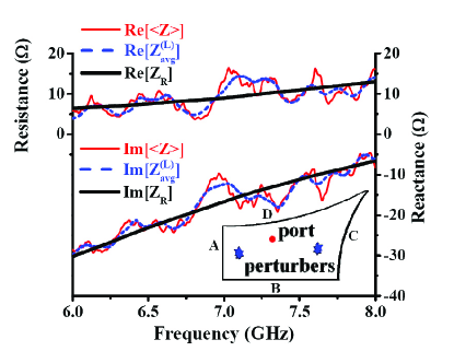
Figure 1: (Color online) Plot of the impedance from the average of 100 cavity realizations $\langle Z\rangle$, versus frequency from 6 to 8 GHz with perturbers inside the cavity. Shown are the real (three upper curves) and the imaginary parts (three lower curves) of the impedance for the theory ($Z^{(L)}_{avg}$ with $L=200$ cm, blue dashed) and the experiment ($\langle Z\rangle$, red solid), as well as the measured radiation impedance of the port ($Z_{R}$, black thick). Inset: The wave chaotic two-dimensional cavity with perturbers and a single port.

To verify that Eq. (2) describes non-universal characteristics of wave-chaotic systems, we first proceed to determine universal statistics by applying the ensemble average. Two irregular-shaped pieces of metal (with the maximum diameters 7.9 cm and 9.5 cm) are added as perturbers in the wave-chaotic system that is shown in the inset of Fig. 1, where the circular dot shows the port and the two starlike objects represent the perturbers. The locations of the two perturbers inside the cavity are systematically changed to produce a set of 100 realizations for the ensemble Sameer . Typically, the shifts of resonances between two realizations are about one mean level spacing. The scattering parameter $S$ is measured from 6 to 18 GHz, covering roughly 1070 modes of the cavity. After the ensemble average, longer ray trajectories have higher probability of being blocked by the two perturbers, and therefore, the main non-universal contributions are due to short ray trajectories. We compare the measured ensemble averaged impedance $\langle Z\rangle$ and the theoretical impedance $Z_{avg}^{(L)}$ that is calculated from Eq. (2) with the sum up to the maximum trajectory length $L=200$ cm, corresponding to a total of 584 trajectories. We multiply each term in the sum, Eq. (2), by a weight equal to the fraction of perturbation configurations that are not intercepted by the trajectory corresponding to that term. The result is shown in Fig. 1 where the three upper curves are the real part of the impedance (resistance) and the three lower curves are the imaginary part (reactance). The experiment curves (red solid) follow the trend of the radiation impedance curves (black thick), and the theory curves (blue dashed) reproduce most of the fluctuations in the experiment curves with only a modest number of trajectories. The good agreement between the measured data and the theoretical prediction verifies that the new theory, Eq. (2), predicts the non-universal features embodied in the ensemble averaged impedance. We believe that the differences between the measured data and the theory are due to the finite number of realizations in the ensemble and diffraction effects that are not taken into account in the theory.

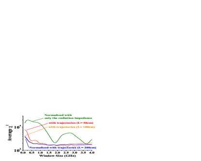
Figure 2: (Color online) The average $\chi^{2}$ of distributions of the phase of the scattering parameter $\varphi_{s}$ on a semi-log scale, where the scattering parameters are calculated from impedance normalized with only the radiation impedance (green) and with ray trajectories according to the maximum trajectory length from $L=50$ cm (red) up to $L=200$ cm (blue), versus frequency window sizes from 0.1 to 4.0 GHz.

We further test our theory by consideration of the statistics of the scattering parameter for an ensemble of perturbation configurations and an ensemble of frequencies. Random matrix theory predicts that, after all non-universal effects have been removed, the resulting scattering parameter, which we denote as $s=(i\xi-1)/(i\xi+1)=|s|e^{i\varphi_{s}}$, should be distributed uniformly in phase in $0\leq\varphi_{s}\leq 2\pi$, and this result is independent of loss, frequency, and mean level spacing Poisson_Kernel_Original ; Henry_paper . The previous work of Refs. S1 ; Sameer ; Sirko removed the non-universal properties by performing normalization with only the radiation impedance, as $i\xi=(Z-iX_{R})/R_{R}$. Here we add ray trajectory corrections based on the maximum trajectory length $L$,

$$i\xi^{(L)}=(Z-iX_{avg}^{(L)})/R_{avg}^{(L)},$$ (3)

and use the $\chi^{2}$ test to evaluate how uniform the resulting phase distributions are. $R_{avg}^{(L)}$ and $X_{avg}^{(L)}$ are the analytic continuations of the real and imaginary parts of $Z_{avg}^{(L)}$ as $k\rightarrow k+ik/(2Q)$ in the experimental case with loss. Experimental distributions of the phase $\varphi_{s}$ of $s$ are calculated from 100 realizations and different frequency windows. $\displaystyle\chi^{2}=\frac{1}{\langle n_{i}\rangle}\sum_{i=1}^{N}(n_{i}-\langle n_{i}\rangle)^{2}$ measures the deviation between the experimental distributions of $\varphi_{s}$ and a perfectly uniform distribution, where $n_{i}$ is the number of elements in the $i^{th}$ bin in the histogram (with ten bins, $N=10$) of the probability of the phase of the scattering parameter $P(\varphi_{s})$, and $\langle n_{i}\rangle$ is the average of $n_{i}$ over $i$. A smaller $\chi^{2}$ value means the experimental data are closer to the theoretical prediction.

Fig. 2 shows the averaged $\chi^{2}$ evaluated over the spectral range from 6 to 18 GHz. The results indicate that the distributions of the measured data are systematically more uniform as more ray trajectories are taken into account in the impedance normalization (Eq. (3)). The improvement is dramatic after including just a few short ray trajectories ($L=50$ cm, 7 trajectories) and saturates beyond $L=100$ cm (36 trajectories). The periodic wiggles represent the effects of the strongest remaining trajectory not taken into account in the theory. Thus, we see that non-universal effects of ray trajectories in the ensemble of wave-chaotic systems can be efficiently removed by considering a few short ray trajectories or by increasing the window size for the frequency ensemble.

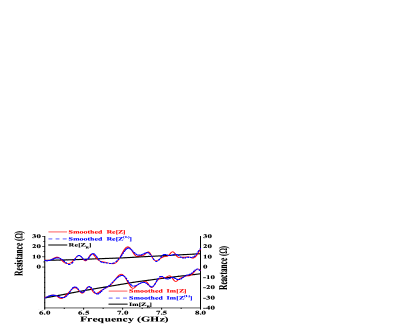
Figure 3: (Color online) Plot of the smoothed impedance versus frequency from 6 to 8 GHz. Shown are the real (three upper curves) and the imaginary part (three lower curves) of the smoothed impedance for the theory ($Z^{(L)}$ with $L=200$ cm, blue dashed) and the experiment (red solid), as well as the measured radiation impedance of the port ($Z_{R}$, black thick).

In addition to experiments with ensemble averaging over perturber positions, we now examine the theory in the stringent case of just a single realization without scatterers, and we use only a frequency ensemble. We consider frequency smoothed experimental data and compare it with the smoothed theoretical prediction. Fig. 3 shows that the smoothed measured impedance $Z$ (red solid) agrees with the smoothed theoretical impedance $Z^{(L)}$ (blue dashed). Notice that $Z_{avg}^{(L)}\rightarrow Z^{(L)}$ because there is only a single realization now. The smoothing function is a Gaussian with standard deviation $\sigma=240$ MHz, which inserts an effective low-pass Gaussian filter on the trajectory length, thus limiting the terms in Eq. (2) to those with a path length $l\lesssim c/\sigma=125$ cm. The results in Fig. 3 shows that the theory correctly captures systematic contributions from short trajectories.

In conclusion, the non-universal effects of coupling and short ray trajectories on wave scattering in chaotic systems are predicted by a newly developed theory Hart and verified experimentally. This is accomplished through statistical tests of the scattering parameter and comparisons of impedance in an ensemble of perturbed systems, as well as a single-realization wave-chaotic system. In particular, non-universal effects have been better considered and removed from measured data to reveal underlying universally fluctuations in the scattering parameter. These results should be useful in many fields, such as nuclear scattering, atomic physics, quantum transport in condensed matter systems, electromagnetics, acoustics, geophysics, etc.

We acknowledge seminal discussions with R. E. Prange and assistance from Michael Johnson. This work was supported by the Air Force Office of Scientific Research Grant No. FA95500710049.

References

- (1) M. C. Gutzwiller, Chaos in Classical and Quantum Mechanics (Springer-Verlag, New York, 1990).
- (2) F. Haake, Quantum Signatures of Chaos (Springer, Berlin, 2000), 2nd ed.
- (3) S. Hemmady, et al., Phys. Rev. Lett. 94, 014102 (2005).
- (4) C. Beenakker, Rev. Mod. Phys. 69, 731 (1997); T. Guhr, A. Müller-Groeling, and H. A. Weidenmüller, Phys. Rep. 299, 189 (1998).
- (5) Y. Alhassid, Rev. Mod. Phys. 72, 895 (2000).
- (6) S. Gnutzmann and U. Smilansky, Adv. Phys. 55, 527 (2006).
- (7) J. A. Hart, T. M. Antonsen, and E. Ott, Phys. Rev. E 80, 041109 (2009).
- (8) F. J. Dyson, J. Math. Phys. 3, 140 (1962).
- (9) P. A. Mello, P. Pereyra, and T. H. Seligman, Ann. Phys. 161, 254 (1985).
- (10) E. Doron and U. Smilansky, Nucl. Phys. A 545, 455 (1992).
- (11) H. U. Baranger and P. A. Mello, Europhys. Lett. 33, 465 (1996).
- (12) P. A. Mello and H. U. Baranger, Waves in Random Media 9, 105 (1999); J. Barthélemy, O. Legrand, and F. Mortessagne, Phys. Rev. E 71, 016205 (2005); J. Barthélemy, O. Legrand, and F. Mortessagne, Europhys. Lett. 70, 162 (2005).
- (13) U. Kuhl, et al., Phys. Rev. Lett. 94, 144101 (2005).
- (14) E. N. Bulgakov, V. A. Gopar, P. A. Mello, and I. Rotter, Phys. Rev. B 73, 155302 (2006).
- (15) Note that consideration of short ray trajectories arises naturally in the semiclassical approach to quantum scattering theory, see C. H. Lewenkopf and H. A. Weidenmüller, Ann. Phys. (N.Y.) 212, 53 (1991); J. Stein and H.-J. Stöckmann, Phys. Rev. Lett. 68, 2867 (1992); J. P. Bird, et al., Phys. Rev. B 52, 14336(R) (1995); H. Ishio and J. Burgdörfer, Phys. Rev. B 51, 2013 (1995); Y.-H. Kim, et al., Phys. Rev. B 68, 045315 (2003); H. Ishio and J. P. Keating, J. Phys. A: Math. Gen. 37, L217 (2004); J. D. Urbina and K. Richter, Phys. Rev. E 70, 015201(R) (2004); R. E. Prange, J. Phys. A: Math. Gen. 38, 10703 (2005); J. D. Urbina and K. Richter, Phys. Rev. Lett. 97, 214101 (2006).
- (16) T. Kottos and U. Smilansky, J. Phys. A: Math. Gen. 36, 3501 (2003).
- (17) Y. V. Fyodorov and D. V. Savin, JETP Lett. 80, 725 (2004); D. V. Savin, H.-J. Sommers, and Y. V. Fyodorov, JETP Lett. 82, 544 (2005); Y. V. Fyodorov, D. V. Savin, and H.-J. Sommers, J. Phys. A 38, 10731 (2005).
- (18) X. Zheng, Ph.D. thesis, University of Maryland (2005), http://hdl.handle.net/1903/2920.
- (19) X. Zheng, T. M. Antonsen, and E. Ott, Electromagnetics 26, 3 (2006); X. Zheng, T. M. Antonsen, and E. Ott, Electromagnetics 26, 37 (2006).
- (20) S. Hemmady, et al., Phys. Rev. E 71, 056215 (2005); S. Hemmady, et al., Phys. Rev. E 74, 036213 (2006); S. Hemmady, et al., Phys. Rev. B 74, 195326 (2006).
- (21) O. Hul, et al., J. Phys. A: Math. Gen. 38, 10489 (2005).