Exploring Case-Control Genetic Association Tests Using Phase Diagrams

Abstract

Backgrounds: By a new concept called “phase diagram”, we compare two commonly used genotype-based tests for case-control genetic analysis, one is a Cochran-Armitage trend test (CAT test at $x=0.5$, or CAT0.5) and another (called MAX2) is the maximization of two chi-square test results: one from the two-by-two genotype count table that combines the baseline homozygotes and heterozygotes, and another from the table that combines heterozygotes with risk homozygotes. CAT0.5 is more suitable for multiplicative disease models and MAX2 is better for dominant/recessive models. Methods: We define the CAT0.5-MAX2 phase diagram on the disease model space such that regions where MAX2 is more powerful than CAT0.5 are separated from regions where the CAT0.5 is more powerful, and the task is to choose the appropriate parameterization to make the separation possible. Results: We find that using the difference of allele frequencies ($\delta_{p}$) and the difference of Hardy-Weinberg disequilibrium coefficients ($\delta_{\epsilon}$) can separate the two phases well, and the phase boundaries are determined by the angle $tan^{-1}(\delta_{p}/\delta_{\epsilon})$, which is an improvement over the disease model selection using $\delta_{\epsilon}$ only. Conclusions: We argue that phase diagrams similar to the one for CAT0.5-MAX2 have graphical appeals in understanding power performance of various tests, clarifying simulation schemes, summarizing case-control datasets, and guessing the possible mode of inheritance.

Introduction

Comparing allele and genotype frequencies of a single marker between the patients and normal people (Sasieni, 1997; Lewis, 2002; Li, 2008) remains the core of a case-control genetic association analysis, prior to a haplotype analysis and bioinformatic analysis to determine the spatial extent and gene context of the signal. The success of a genetic association study crucially depends on study design (Amos, 2007), but the choice of test is also somewhat important. If we focus on genotype-based tests, i.e., each observed genotype is a sample instead of two allele samples (Sasieni, 1997), there are many possible types of tests to choose from. For example, the Pearson’s goodness-of-fit test on the 2-by-3 genotype count table, Cochran-Armitage trend (CAT) tests with a single parameter value $x$ which determines the relative risk of heterozygote with respect to the two homozygotes (Sasieni, 1997; Devlin and Roeder, 1999; Slager and Schaid, 2001), tests that are maximized over two or more tests (Yamada et al., 2001; Freidlin et al., 2002; Tokuhiro et al., 2003; Zheng et al., 2006a), and those that stepwisely use a few tests sequentially (Zheng et al., 2008). This quote from (Balding, 2006) might capture the feeling about the current state: “there is no generally accepted answer to the question of which single-(marker) test to use” in genetic case-control association analysis. The widespread use of whole-genome association in the study of complex diseases nowadays (Wellcome Trust Case Control Consortium, 2007) adds an urgency in having a better understanding of this issue.

If one statistical test is always more powerful than another test, the first test should of course be used all the time. However, each test may have its own strength and weakness depending on the true underlying model. For example, Cochran-Armitage trend as a family of tests is to test the equality of genotype frequencies in the case and the control group, but as a test at a parameter $x$ is to test the null hypothesis $P_{case}(AA)+xP_{case}(Aa)=P_{control}(AA)+xP_{control}(Aa)$ ($AA$ is the risk genotype, and $P(AA)$ is its frequency; similarly for heterozygous genotype $Aa$). The CAT test at $x=0$ is most powerful for detecting recessive disease genes, whereas it is more powerful at $x=0.5$ when Hardy-Weinberg equilibrium (HWE) holds for case and control groups. For a pair of tests, in the space of all possible disease models, the first test can be more powerful in some regions whereas the second test is more powerful in other regions. This simple picture is reminiscent of the phase diagram in physics (e.g., Gibbs, 1873; Lifshitz and Landau, 1980) where a phase can be solid, liquid or gas depending on the temperature, pressure, or other relevant quantities. In our case-control genetic test example, the aim of phase diagram is to graphically depict regions where specific test is more powerful than others. Note that one should not confuse the usage of “phase” here with the meaning often used in genetics, i.e., of the “parental origin” of an allele in a genotype (e.g. Scheet and Stephens, 2006).

Although the principle of our phase diagram can be established as discussed above, there are several practical considerations. First, a disease model is specified by many parameters, and one may wonder whether the phase structure can be seen in a two-dimensional space. Second, if the two phases are highly intermingled in one parameterization, we may ask if other parameterization schemes are better suited for separating the two phases. Third, besides the definition of phases which are based on statistical power, we can also define phases that are based on $p$-value, and the question is whether the two ways of defining phase diagrams are similar. This paper uses a specific pair of tests to address these questions and to show the utility of this approach.

The motivation of our study is to discuss the issue of in what circumstances, one should use a particular test instead of others. We first study the parameterization of phase diagram, then construct two phase diagrams, one power-based and another $p$-value-based, for a pair of commonly used tests. The phase boundary in both versions of phase diagram will be determined. And we examine several whole-genome association datasets using the phase diagram. Several other applications of the phase diagram are also discussed, including comparison of two random simulations of disease models, and graphical display of case-control data of many SNPs.

Methods

Case-control difference of allele frequency and Hardy-Weinberg disequilibrium (HWD) coefficient given a disease model

A single-locus biallelic disease model can be specified by four parameters: three penetrances $f_{i}=$Prob(disease$|G_{i}$) ($i=0,1,2$) where $\{G_{i}\}$ are the three genotypes $aa,aA,AA$, and the population $A$-allele frequency $p$. Alternatively, one can use the allele frequency $p$, two relative genotype risks $\lambda_{i}=f_{i}/f_{0}$ ($i=1,2$), and disease prevalence $K=f_{0}[(1-p)^{2}+2p(1-p)\lambda_{1}+p^{2}\lambda_{2}]$ to specify the disease model. Denote $A$-allele frequency in case and control group as $p_{1}$ and $p_{0}$, and HWD coefficient (Weir, 1996) in case and control group as $\epsilon_{1}$ and $\epsilon_{0}$; all four ($p_{1},p_{0},\epsilon_{1},\epsilon_{0}$) can be derived from a given disease model, under the assumption that HWE holds true for the general population that contains both cases and controls (Wittke-Thompson et al., 2005). We use the difference of $A$-allele frequency ($\delta_{p}$) and the difference of HWD coefficients ($\delta_{\epsilon}$) in case and control group as the parameters for our phase diagram:

$$\delta_{p}\equiv p_{1}-p_{0} = \frac{f_{0}(p^{2}\lambda_{2}+p(1-p)\lambda_{1})}{K}-\frac{p^{2}(1-f_{0}\lambda_{2})+p(1-p)(1-f_{0}\lambda_{1})}{1-K}$$

$$\delta_{\epsilon}\equiv\epsilon_{1}-\epsilon_{0} = \frac{f_{0}^{2}p^{2}(1-p)^{2}(\lambda_{2}-\lambda_{1}^{2})}{K^{2}}-\frac{f_{0}p^{2}(1-p)^{2}(2\lambda_{1}-1-\lambda_{2}-f_{0}\lambda_{1}^{2}+f_{0}\lambda_{2})}{(1-K)^{2}}$$

When $\lambda_{1}>1$ and $\lambda_{2}>1$, $A$-allele is enriched in the case group, and $\delta_{p}$ is always positive. On the other hand, if $\lambda_{1}<1$ and $\lambda_{2}<1$, $A$-allele is depleted in the case group and $\delta_{p}$ is negative. To be consistent, we call $A$ the risk allele when $\delta_{p}>0$. Whether $A$-allele is a minor allele ($p<0.5$) or a major allele ($p>0.5$) does not by itself affect the sign of $\delta_{p}$ and $\delta_{\epsilon}$.

Case-control difference of allele frequency and Hardy-Weinberg disequilibrium coefficient given a genotype count table

Table 1(A) shows a case-control genotype count table $\{N_{ij}\}$ ($i=$1,0 for case, control, and $j=$0,1,2 for genotypes with 0, 1, 2 copies of allele $A$) with total $N=N_{1}+N_{0}$ samples. The same table is parameterized in Table 1(B) using the estimated $\{\hat{p}_{i}\}$ and $\{\hat{\epsilon}_{i}\}$ ($i=$1,0 for case, control). The estimated $A$-allele frequency ($\hat{\delta}_{p}$) and the estimated difference of HWD coefficients ($\hat{\delta}_{\epsilon}$) in case and control group can be obtained from Table 1(A) as:

$$\hat{\delta}_{p} = \hat{p}_{1}-\hat{p}_{0}=\frac{N_{11}/2+N_{12}}{N_{1}}-\frac{N_{01}/2+N_{02}}{N_{0}}$$

$$\hat{\delta}_{\epsilon} = \hat{\epsilon}_{1}-\hat{\epsilon}_{0}=\frac{N_{12}}{N_{1}}-\left(\frac{N_{11}/2+N_{12}}{N_{1}}\right)^{2}-\frac{N_{02}}{N_{0}}+\left(\frac{N_{01}/2+N_{02}}{N_{0}}\right)^{2}$$ (2)

For notation simplicity, the hat ($\hat{}$) will be removed later on, and whether the model-based or data-based usage is applied should be clear from the context.

Note that switching the $A$ and $a$ allele, or equivalently, switching the first and the third column in Table 1, changes the sign of $\delta_{p}$, whereas the sign of $\delta_{\epsilon}$ is unaffected. Eq.(Case-control difference of allele frequency and Hardy-Weinberg disequilibrium coefficient given a genotype count table) also shows another advantage of using the difference of two HWD coefficients: if the disequilibrium is sensitive to typing errors, its effect is minimized when the difference $\hat{\delta}_{\epsilon}$ is used.

Cochran-Armitage trend test and MAX2 test

Cochran-Armitage trend (CAT) test at parameter $x$ assigns a score of 0, $x$, and 1 for genotypes $aa$, $aA$, and $AA$, for log-risk relative to the baseline $aa$ genotype (Sasieni, 1997; Devlin and Roeder, 1999; Slager and Schaid, 2001). Sometimes, the name of Cochran-Armitage trend test is used to only refer to that at parameter $x=0.5$ (Balding, 2006), which we will call as CAT0.5. On the other hand, CAT at parameter settings of $x=0$ and $x=1$ is equivalent to assuming recessive and dominant models, which we will refer to as CAT0 and CAT1.

With the genotype count in Table 1, the test statistic of CAT0.5, CAT0, and CAT1 can be derived (see, e.g., Sasieni, 1997). We re-parameterize these test statistics using a new set of parameters including $\delta_{p}$ and $\delta_{\epsilon}$:

$$X^{2}(CAT0.5) = \frac{N_{1}N_{0}}{N}\cdot\frac{2\delta_{p}^{2}}{\overline{p}+\overline{p^{2}}-2\overline{p}^{2}+\overline{\epsilon}}$$

$$X^{2}(CAT0) = \frac{N_{1}N_{0}}{N}\cdot\frac{(2\stackrel{{\scriptstyle=}}{{p}}\delta_{p}+\delta_{\epsilon})^{2}}{(\overline{p^{2}}+\overline{\epsilon})(1-\overline{p^{2}}-\overline{\epsilon})}$$

$$X^{2}(CAT1) = \frac{N_{1}N_{0}}{N}\cdot\frac{(2(1-\stackrel{{\scriptstyle=}}{{p}})\delta_{p}-\delta_{\epsilon})^{2}}{(2\overline{p}-\overline{p^{2}}-\overline{\epsilon})(1-2\overline{p}+\overline{p^{2}}+\overline{\epsilon})}$$ (3)

where $\delta_{p}\equiv p_{1}-p_{0}$, $\overline{p}\equiv(N_{1}/N)p_{1}+(N_{0}/N)p_{0}$, $\overline{p^{2}}\equiv(N_{1}/N)p_{1}^{2}+(N_{0}/N)p_{0}^{2}$, $\overline{\epsilon}\equiv(N_{1}/N)\epsilon_{1}+(N_{0}/N)\epsilon_{0}$, $\stackrel{{\scriptstyle=}}{{p}}\equiv(p_{1}+p_{0})/2$. CAT0.5 usually leads to very similar result to the allele-based test. But since CAT0.5 is a genotype-based test, it does not have the problem of allele-based test for artificially doubling the sample size (Sasieni, 1997).

The MAX2 test is defined by the maximization of the CAT0 and CAT1 test statistics: $X^{2}(MAX2)\equiv\max(CAT0,CAT1)$. Although MAX2 has been used in a few analyses (e.g., Yamada et al., 2001; Tokuhiro et al., 2003), it did not have a formal name. The name of MAX2 used here is to distinguish it from the MAX3 test ($\max(CAT0,CAT1,CAT0.5)$) proposed in (Freidlin et al., 2002).

Since MAX2 involves a multiple testing whereas CAT0.5 does not, its $p$-values are calculated differently. For CAT0.5, the $p$-value is simply derived by the $\chi^{2}$ distribution with 1 degree of freedom. For MAX2, Dunn-S̆idák multiple testing correction (Ury, 1976) is exact if CAT0 and CAT1 test statistics were independent:

$$p_{MAX2} = P_{0}(X^{2}(MAX2)>T)=1-P_{0}(X^{2}(MAX2)<T)=1-P_{0}(X^{2}<T)^{2}$$ (4)

$$= 1-(1-p_{X2})^{2}=2p_{X2}-p_{X2}^{2}$$

where $P_{0}$ is the null distribution, $p_{X2}$ is the $p$-value for a $\chi^{2}$-distributed test statistic. In R code (http://www.r-project.org/), the command for calculating $p$-value for MAX2 is 1-pchisq(MAX2, df=1)^2.

For dataset generated by a known disease model, CAT test statistics follow chi-square distributions with non-central parameters. The non-central parameters for CAT0.5, CAT0 and CAT1 are given in Eq.(Cochran-Armitage trend test and MAX2 test), only that $\delta_{p}$, $\delta_{\epsilon}$, and other parameters are determined by the disease model, not from the data. Alternatively, power can be determined empirically by simulation.

Simulation

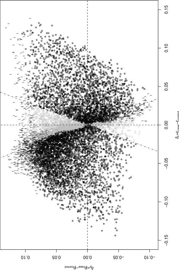
Figure 2: The CAT0.5-MAX2 phase digram, with $\delta_{\epsilon}=\epsilon_{1}-\epsilon_{0}$ (difference of two HWD coefficients in case and control group) as the $x$-axis, and $\delta_{p}=p_{1}-p_{0}$ (difference of allele frequencies in case and control group) as the $y$-axis, determined by comparing the empirical power of CAT0.5 and MAX2 tests. More than 10000 disease models are randomly sampled, each is used to randomly generate 5000 replicates of 500 cases and 500 controls. The empirical power of CAT0.5 and MAX2 based on these 5000 replicates are compared when the type I error is controlled at 0.05. A black circle is drawn when the empirical power of MAX2 is larger than that of CAT0.5, and a gray circle when CAT0.5 is more powerful than MAX2. If the empirical powers of both tests are larger than 0.99, a symbol “1” is marked. The two dashed lines form angles of 73.125^∘ and 106.875^∘ ($13\pi/32$ and $19\pi/32$) with the $x$-axis, or, $\pm 16.875^{\circ}$ ($3\pi/32$) with the $y$-axis.

For empirical power calculation, we sampled $N_{r}$ (=5000) replicates of genotypes for $N_{case}$ (=500) cases and $N_{control}$ (=500) controls, given a disease model. In Fig.2, $N_{m}$ (=10000) disease models were generated randomly. The relative genotype risks $\lambda_{1}$ and $\lambda_{2}$ are randomly selected from a range (e.g., (0.5-2)), and the population $A$-allele frequency is randomly selected (e.g., from (0.1-0.9)). The type I error is set at 0.05 and we have determined the test statistic threshold for MAX2 either by permutation or by Dunn-S̆idák formula. Due to the consistency between the two approaches, the type I error is controlled mostly by using the Dunn-S̆idák formula in Eq.(4). The empirical power of CAT0.5 or MAX2 at the given type I error is determined by the proportion of replicates that exceeds the threshold.

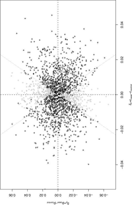
Figure 4: The CAT0.5-MAX2 phase diagram based on $p$-value of two tests. 2000 genotype count tables are simulated using the null model with 500 cases and 500 controls, and $A$-allele frequency being samples from the range of ($10^{-5}$-0.5). If the $p$-value by MAX2 is smaller (larger) than that by CAT0.5, a black (grey) circle is drawn. The two dashed lines are the same as those in Fig.2, with angles of 73.125^∘ and 106.875^∘ ($13\pi/32$ and $19\pi/32$) with the $x$-axis.

For the phase diagram in Fig.4 under the null model (i.e., same allele and genotype frequency according to the HWE), $N_{r}$ (=2000) replicates of genotype were generated for $N_{case}$ (=500) cases and $N_{control}$ (=500) controls.

Results

Phase diagrams based on power given the disease model

In the $\delta_{\epsilon}$-$\delta_{p}$ space, known types of disease models such as dominant, recessive, additive, multiplicative, and over-dominant models fall in different regions of the plane, after requiring the risk allele $A$ to have higher frequency in cases than in controls, as can be seen from Fig.1. For example, recessive models reside in the first quadrant, additive, dominant, over-dominant models are in the second quadrant, and the multiplicative models sit along the $y$-axis.

We pick CAT0.5 and MAX2 as the two tests to compare for the following reasons. First, allele-based test is still one of the most commonly used tests in case-control genetic analysis, and we would like to choose a similar genotype-based test. Second, we want to choose a test that is robust against disease model mis-specification. These two considerations lead to CAT0.5 and MAX2. Fig.2 shows the power-based CAT0.5-MAX2 phase diagram, where empirically obtained statistical power of CAT0.5 and MAX2 are compared while controlling the type I error, in the space parameterized by $\delta_{\epsilon}$ and $\delta_{p}$.

The region in Fig.2 where power(MAX2) $>$ power(CAT0.5), or phase 1, covers most of the model space. On the other hand, region where power(CAT0.5) $>$ power(MAX2), or phase 2, is limited to a narrow angle around the $y$-axis. For regions far away from the $x$-axis, both tests lead to close to 100% power (the symbol “1” is used to mark the points when both power(CAT0.5) and power(MAX2) are larger than 0.99). The phase boundary in the first (and the third) quadrant can be roughly approximated by the line $\theta=tan^{-1}(\delta_{p}/\delta_{\epsilon})=73.125^{\circ}$ ($13\pi/32$). The phase boundary in the second (and the fourth) quadrant is not sharp with some degree of overlap between the two phases. However, the line $\theta=tan^{-1}(\delta_{p}/\delta_{\epsilon})=106.875^{\circ}$ ($19\pi/32$) seems to provide a reasonable boundary to phase 2 points.

The phase structure presented in Fig.2 is consistent with our current knowledge that allele-based test and CAT0.5 are most powerful for multiplicative models. In fact, it can be shown that non-central parameter in the $\chi^{2}$ distribution for the allele-based test is strictly larger than that of either CAT0 or CAT1 (i.e., either one of two ways to combine heterozygote counts with the homozygote counts), if (1) $\epsilon_{1}=\epsilon_{0}=0$ and (2) $N_{1}=N_{0}$ (Suh and Li, 2007). However, it was somewhat surprising that the two phases in Fig.2 are not separated by vertical lines. The two-phase genetic model selection method proposed in (Zheng and Ng, 2008) attempts to infer the underlying disease model by $\delta_{\epsilon}$ value alone. Here we show that the model selection could be more accurate if both $\delta_{\epsilon}$ and $\delta_{p}$ parameters are considered.

To have a better understanding of the phase structure, in Fig.3, we plot the power of CAT0.5 as a function of $|\delta_{p}|$ as well as power of MAX2 as a function of radius $\sqrt{\delta_{p}^{2}+\delta_{\epsilon}^{2}}$. As expected, the power of CAT0.5 increases as the allele frequency difference is larger, because CAT0.5 is very close to the allele-based test which is designed to detect allele frequency differences. On the other hand, it was unexpected that the power of MAX2 increases with the radius, and the increase follows a similar way as power of CAT0.5 increases with $|\delta_{p}|$. If we draw the two plots in one, the two more or less overlap. In a crude approximation, suppose power(CAT0.5) vs. $|\delta_{p}|$ and power(MAX2) vs. $\sqrt{\delta_{p}^{2}+\delta_{\epsilon}^{2}}$ follow the same functional form, then the power of MAX2 should be larger than that of CAT0.5 over the whole plane except the $y$-axis, because radius is always larger than the $y$ value except for the $y$-axis. Although this is only an approximation, Fig.3 helps us to understand why the robust MAX2 test is more likely to be more powerful than the CAT0.5 test in the space of all possible models.

Phase diagrams based on $p$-values given the genotype data

Power analysis is always discussed in a theoretical context because it requires our knowing of the true disease model. In reality, the disease model is not supposed to be known. Towards a data-driven concept of phase diagram, we define the following phase diagram based on $p$-values.

As can be seen from Eq.(Cochran-Armitage trend test and MAX2 test), the relative magnitude of CAT0.5 and MAX2 test statistics depends on the estimated value of four parameters $p_{1},p_{0},\epsilon_{1},\epsilon_{0}$, as the common factor $N_{1}N_{0}/N$ is canceled out. If we assume that averaged quantities such as $\overline{p}$ and $\overline{\epsilon}$ do not vary dramatically with different $p_{1},p_{0},\epsilon_{1},\epsilon_{0}$ values, then the relative magnitude of CAT0.5 and MAX2 test statistics are mainly determined by the parameters $\delta_{p}$ and $\delta_{\epsilon}$.

Because of the multiple testing in MAX2, even if a MAX2 test statistic is larger than that of CAT0.5, the MAX2 $p$-value may not be smaller than the $p$-value by CAT0.5. It should be noted that the assumption to apply Dunn-S̆idák formula in Eq.(4), i.e., the independence between the two terms to be maximized, does not hold exactly. However, the correlation between CAT0 and CAT1 is actually small. It was shown in (Freidlin et al., 2002; Zheng et al., 2006a) that the correlation between CAT0 and CAT1 test statistics under the null hypothesis ($p_{1}=p_{0}$), if HWE is true, is $\sqrt{p_{1}(1-p_{1})/[(1+p_{1})(2-p_{1})]}$. This correlation is at most 1/3 which is reached when $p_{1}=p_{0}=0.5$. Simulation shows that Dunn-S̆idák formula leads to an accurate estimation of $p_{MAX2}$, despite a weak violation of the assumption. This is in a contrast with MAX3, where the correlation between CAT0.5 and either CAT1 or CAT0 is too strong to apply the Dunn-S̆idák formula (González et al., 2008; Li et al., 2008).

Fig.4 shows the phase diagram based on comparing $p$-values of CAT0.5 and MAX2 when genotype count tables are randomly sampled from the null model. The MAX2 (CAT0.5) test is preferred over CAT0.5 (MAX2) in phase 1 (2) because it has a smaller $p$-value (black (grey) dots). When we draw the same straight lines as Fig.2 with 73.125^∘ and 106.875^∘, a similar observation can be made that the phase separation is much better in the first (and the third) quadrant, and a low level of overlap occurs in the second (in the fourth) quadrant. We conclude that the CAT0.5-MAX2 phase diagram based on $p$-values is very similar to the CAT0.5-MAX2 phase diagram based on power. Because the ranges of $x$ and $y$ in Fig.4 are smaller than those in Fig.2, another understanding of $p$-value-based phase diagram is that it is the “extension” of power-based phase diagram towards the origin.

Illustration of the CAT0.5-MAX2 phase digram by results of several genome-wide association studies

Recently, the largest scale whole-genome association study was carried out by Wellcome Trust Case Control Consortium on several common complex diseases (Wellcome Trust Case Control Consortium, 2007). We take the genotype count for SNPs that showed the strongest, and for many of them, validated association signal using extra samples, to illustrate the use of phase diagram. The association signal in (Wellcome Trust Case Control Consortium, 2007) s mainly ranked by the CAT0.5 test.

Table 2(A) lists the raw genotype count data of 11 SNPs that are associated with one of these diseases: ankylosing spondylitis (Wellcome Trust Case Control Consortium & Australo-Anglo-American Spondylitis Consortium, 2007), type 1 diabetes (Todd et al., 2007), Crohn’s disease (Parkes et al., 2007), and type 2 diabetes (Zeggini et al., 2007). Table 2(B) shows the estimated case or control minor allele frequency ($p_{1},p_{0}$) and their difference ($\delta_{p}$), case or control HWD coefficients ($\epsilon_{1},\epsilon_{0}$) and their difference ($\delta_{\epsilon}$), the angle $\theta$ in the $\delta_{p}-\delta_{\epsilon}$ phase diagram with respect to either $x$ or $y$ axis, and CAT test statistics at $x=0.5,0,1$.

There are several observations made from Table 2(B). As expected, the estimated HWD coefficient in case group $\epsilon_{1}$ is usually larger in magnitude than that in control group $\epsilon_{0}$. However, the largest observed $\epsilon_{1}$ is only around 0.01. On the other hand, allele frequency difference is large (0.03-0.07) due to the fact that these SNPs are selected by significant CAT0.5 test. A consequence of the two facts is that the angle with respect to the $y$-axis in Table 2(B) tends to be small, with the exception of SNP rs27044 which is associated with ankylosing spondylitis ($\theta-90^{\circ}=16.4^{\circ}$).

The closeness to the $y$ axis of these SNPs on the phase diagram should indicate, on average, CAT0.5 test to be better than MAX2 test. Indeed, the $X^{2}$(CAT0.5) test statistics are larger than $X^{2}$(MAX2) except for two SNPs: rs27044 and rs2542151. It is not surprising to see rs27044 in the exception list as it has the largest angle with respect to the $y$-axis, and the negative sign of $\delta_{\epsilon}$ indicates that the disease model for rs27044 is more likely dominant. For rs27044, MAX2 test leads to a more significant result ($p$-value = 1.8 $\times 10^{-7}$) than the CAT0.5 test ($p$-value= 10^-6). For rs2542151, its position in the phase diagram forms a smaller angle with the $y$-axis than the rs27044 SNP (8.5^∘ vs. 16.4^∘), but the angle is still large enough such that MAX2 leads to a more significant test ($p$-value =$3.7\times 10^{-14}$) than CAT0.5 test ($p$-value = $1.9\times 10^{-13}$).

Discussion and conclusions

Our choice of $\delta_{p}$ is to capture the linear or first-order term from the disease model or data, and $\delta_{\epsilon}$ to capture the nonlinear or second-order term. In quantitative genetics, there is a similar approach in using the additive variance $\sigma_{a}^{2}$ and dominance variance $\sigma_{d}^{2}$ (Fisher, 1918; Falconer and Mackay, 1996). When these concepts from quantitative genetics are translated to dichotomous traits, $\sigma_{a}^{2}=2p(1-p)(p(f_{2}-f_{1})+(1-p)(f_{1}-f_{0}))^{2}$, and $\sigma_{d}^{2}=p^{2}(1-p)^{2}(f_{2}+f_{0}-2f_{1})^{2}$ (see, e.g., Blackwelder and Elston, 1985). Using Eq.(Case-control difference of allele frequency and Hardy-Weinberg disequilibrium (HWD) coefficient given a disease model), we have

$$\delta_{p} = \frac{f_{2}-K}{K(1-K)}p^{2}+\frac{f_{1}-K}{K(1-K)}p(1-p)$$ (5)

$$= \frac{pf_{2}+(1-p)f_{1}-K}{K(1-K)}\cdot p=\frac{p(f_{2}-f_{1})+q(f_{1}-f_{0})}{K(1-K)}\cdot p(1-p).$$

In other words, the square of our first-order parameter $\delta_{p}^{2}$ is proportional to the additive variance $\sigma_{a}^{2}$. Similarly, using Eq.(Case-control difference of allele frequency and Hardy-Weinberg disequilibrium (HWD) coefficient given a disease model) for $\delta_{\epsilon}$, we have

$$\delta_{\epsilon} = p^{2}(1-p)^{2}\left(\frac{1}{K^{2}}-\frac{1}{(1-K)^{2}}\right)(f_{2}f_{0}-f_{1})+\left(\frac{p(1-p)}{1-K}\right)^{2}(2f_{1}-f_{2}-f_{0})$$ (6)

$$= \frac{p^{2}(1-p)^{2}(1-2K)}{K^{2}(1-K)^{2}}(f_{2}f_{0}-f_{1}^{2})+\frac{p^{2}(1-p)^{2}}{(1-K)^{2}}(f_{2}+f_{0}-2f_{1}).$$

When the disease prevalence $K$ is low, $\delta_{\epsilon}$ is roughly proportional to $f_{2}f_{0}-f_{1}^{2}$, as versus the $f_{2}+f_{0}-2f_{1}$ expression in $\sigma_{d}^{2}$. Actually, the HWD coefficient in the control group, which is small, is proportional to the difference between $f_{2}f_{0}-f_{1}^{2}$ and $f_{2}+f_{0}-2f_{1}$, and two are approximately equal when $\lambda_{1},\lambda_{2}$ are small (Zheng et al., 2006b). Crudely, the square of $\delta_{\epsilon}$ can be said to be proportional to the dominance variance $\sigma_{d}^{2}$.

The idea to use the test that is most powerful to the underlying model sounds straightforward, but in reality the true disease model is unknown. There have been attempts to infer the disease model by the HWD information. For example, (Wittke-Thompson et al., 2005) distinguishes HWD from different disease models and proposed its use for data fitting (note that the additive model defined in (Wittke-Thompson et al., 2005), $\lambda_{2}=2\lambda_{1}$, is different from that defined here, $f_{2}-f_{1}=f_{1}-f_{0}$ or $\lambda_{2}=2\lambda_{1}-1$). In (Zheng and Ng, 2008), the signs of $\epsilon_{1}$ and $\epsilon_{0}$ are used for genetic model selection: (+,$-$) for recessive models, ($-$,+) for dominant models, and ($-$,$-$) for multiplicative and additive models. Since the amount of HWD in control group is usually much smaller than that in case group, the sign of $\delta_{\epsilon}=\epsilon_{1}-\epsilon_{0}\approx\epsilon_{1}$ may serve the purpose in selecting recessive and dominant models. All these previous works use HWD alone in genetic model selection, without considering a joint effect of HWD and allele frequency difference.

The result discussed in this paper shows that a joint consideration of $\delta_{\epsilon}$ and $\delta_{p}$ could be more effective, than a consideration of $\delta_{\epsilon}$ only, in selecting disease model. The following simple procedure might be reasonable: first draw a line from origin to the data-determined $(x,y)=(\delta_{\epsilon},\delta_{p})$ position, then calculate the angle formed by this line and the $y$-axis. If the angle is smaller than 3$\pi$/32 (or 16.875^∘), the underlying model is more likely to be multiplicative and CAT0.5 is the preferred test to use. On the other hand, if the angle with respect to the $y$-axis is larger, the underlying model is more likely to be recessive (if it’s in the first quadrant) or dominant (second quadrant), and MAX2 is preferred over CAT0.5. A caution on this procedure is that, unless the sample size is very large and unless the true model is away from the phase transition line, the disease model can still be incorrectly inferred.

Comparing the power of two tests is always tricky because the answer depends on what is known about the true model. It is very much in the spirit of Bayesian statistics that the posterior probability distribution depends on the prior. Any claim on discovering a more powerful test may contain a caveat on how the alternative model is sampled. Phase diagram discussed here provides a framework to visually inspect distributions on the $\delta_{p}$-$\delta_{\epsilon}$, for the simulated models,

Fig.5 shows the distribution on the phase diagram of two different ways of simulating genotype count tables. The first is by randomly sampling two allele frequencies $p_{case}$ and $p_{control}$ that are close to each other (difference is less than 0.1), then the genotype frequencies in the model are determined by the HWE. One such model is used to generate one replicate dataset and $\delta_{\epsilon}$, $\delta_{p}$ values are determined from the replicate. The second way to generate a random model is to randomly sample two sets of genotype frequencies, for case and control group, that are close to each other (difference is less than 0.1), and that model is used to simulate one replicate dataset.

When we compare the empirical power of MAX2 and MAX3, MAX3 is more powerful than MAX2 in the first simulation, whereas MAX2 is slightly more powerful than MAX3 in the second simulation. The phase diagram in Fig.5 easily solves the puzzle: from Fig.5, it can be seen that simulated datasets by the first method centered around the $y$-axis, as genotype frequencies in the model are obtained by HWE, whereas those by the second method are more widespread in the $x$-axis. If we require a graphic showing of the phase diagram like Fig.5 in any power comparison between two tests, there would be less misunderstanding of seemingly conflicting empirical results.

The phase-diagram can also be used to summarize a case-control dataset with many SNPs. Fig..6 shows 2147 SNPs on chromosome 18q21 for 460 cases and 459 controls used in Genetic Analysis Workshop 15 (Amos et al., 2007; Wilcox et al., 2007), with $\hat{\delta}_{p}$ and $\hat{\delta}_{\epsilon}$ calculated by Eq.(Case-control difference of allele frequency and Hardy-Weinberg disequilibrium coefficient given a genotype count table). These SNPs are filtered from the original list of 2719 SNPs by requiring no more than 10 missing typings and minor allele frequency to be larger than 0.05. For some SNPs, alleles are switched to make sure $\delta_{p}$ is positive. One striking visual impression of Fig.6 is that the SNPs with the largest $\delta_{p}$ values are not located on $y$-axis, but in the first quadrant, indicating that recessive model better describes the effect of these SNPs than the multiplicative model.

In Fig.6, the SNP rs3745064 at position 53.305Mb exhibits the largest $\delta_{p}$ value (=0.076) (Kuo et al., 2007; Tapper et al., 2007). The distribution of case samples among the three genotypes is 37, 180, 243, and that of control samples is 50, 223, 186, leading to $p_{1}=0.724$, $p_{0}=0.648$, $\delta_{1}=0.0042$, $\delta_{0}=-0.015$. For this SNP, we expect the largest test statistic value to be CAT($x=0$) because it is located in the first quadrant on the phase diagram. Indeed, CAT($x=0$)=13.97, CAT($x=0.5$)=12.47, CAT($x=1$)=2.18, and MAX2 test statistic is more powerful than CAT($x=0.5$).

Using the phase diagram to examine the most recent whole-genome association data shows that SNPs with the strongest association signal tend to be multiplicative, and CAT0.5 test is more powerful than MAX2 test in this situation. However, we should not exclude the possibility that it is due to a selection bias, as the top ranking genes were chosen by CAT0.5 test result. Also, if the most significant SNPs exhibit larger allele frequency differences, whereas their $\delta_{\epsilon}$ value is limited, their positions in the phase diagram is expected to be closer to the $y$-axis.

Whether the result in Table 2(B) is due to selection bias or not, our approach could be useful in analyzing whole-genome association data, as illustrated by Fig.6. Applying MAX2 may change the rank order of some SNPs that are near the top, and consequently change the pool of SNPs to be studied further. If MAX2 test does improve the $p$-value over CAT0.5 for a SNP, one can check whether the HWD mainly occurs in the case instead of the control group. The location of a SNP on the phase diagram provides a quick filtering of SNPs where the inclusion of non-multiplicative models may improve the association signal, such as the example of rs3745064 on Fig.6. Due to a high cost of typing extra samples in validating the associated SNPs for the second round, it is important to carry out careful analyses including the consideration of alternative disease models.

In conclusion, using the phase diagram is to partition the violation of null hypothesis of equal genotype frequency in case and control groups into two components, one $\delta_{p}$ for allele frequency difference and another $\delta_{\epsilon}$ for difference in HWD coefficients. The relative magnitude of $\delta_{p}$ and $\delta_{\epsilon}$ determines which test, e.g., between CAT0.5 and MAX2, is more powerful. The phase diagram highlights the point that no uniformly powerful test exists, and a test is only more powerful regionally in the model space. We believe the use of phase diagram can aid the design of test when some knowledge of the mode of inheritance is available, as well as inferring the underlying mode of inheritance from the data.

REFERENCES

Amos CI (2007). Successful design and conduct of genome-wide association studies, Hum. Mol. Genet., 16, R220-R225.

Amos CI, Chen WV, Remmers E, Siminovitch KA, Seldin MF, Criswell LA, Lee AT, John S, Shephard ND, Worthington J, Cornelis F, Plenge RM, Begovich AB, Dyer TD, Kastner DL, Gregersen PK (2007). Data for Genetic Analysis Workshop (GAW) 15 Problem 2, genetic causes of rheumatoid arthritis and associated traits, BMC Proc., 1(suppl 1), S3.

Balding DJ (2006). A tutorial on statistical methods for population association studies. Nat. Rev. Genet., 7,781-791.

Blackwelder WC, Elston RC (1985). A comparison of sib-pair linkage tests for disease susceptibility loci, Genet. Epid., 2, 85-97.

Devlin B & Roeder K (1999). Genomic control for association studies. Biometrics, 55,997-1004.

Falconer DS, Mackay TFC (1996). Introduction to Quantitative Genetics, 4th edition, (Benjamin Cummings).

Fisher RA (1918). The correlation between relatives on the supposition of Mendelian inheritance, Phil Tran Royal Soc Edinburgh, 52, 399-433.

Freidlin B, Zheng G, Li Z, Gastwirth JL (2002). Trend tests for case-control studies of genetic markers, power, sample size and robustness. Hum. Heredity, 53,146-152.

Gibbs JW (1873). Graphical methods in the thermodynamics of fluids, Transactions of Connecticut Academy of Arts and Science, 2(11), 309-342; A method of geometrical representation of the thermodynamic properties of substances by means of surfaces, ibid., 2(14), 382-404.

González JR, Carrasco JL, Dudbridge F, Armengol L, Estivill X, Morento V (2008). Maximizing association statistics over genetic models, Genet. Epid., 32, 246-254.

Kuo TY, Lau W, Hu C, Zhang W (2007). Association mapping of susceptibility loci for rheumatoid arthritis, BMC Proc., 1(Suppl 1), S15.

Lewis CM (2002). Genetic association studies, design, analysis and interpretation. Brief. Bioinformatics, 3,146-153.

Li Q, Zheng G, Li Z, Yu K (2008). Efficient approximation of p-value of the maximum of correlated tests, with applications to genome-wide association studies, Ann. Hum. Genet., 72, 397-406.

Li W (2008). Three lectures on case-control genetic association analysis. Brief. Bioinformatics, 9,1-13.

Lifshitz EM & Landau LD (1980). Statistical Physics, Course of Theoretical Physics, Volume 5, 3rd edition (Butterworth-Heinemann).

Parkes M, Barrett JC, Prescott NJ, Tremelling M, Anderson CA, Fisher SA, Roberts RG, Nimmo ER, Cummings FR, Soars D (2007). Sequence variants in the autophagy gene IRGM and multiple other replicating loci contribute to Crohn’s disease susceptibility. Nat. Genet., 39,830-832.

Sasieni PD (1997). From genotypes to genes, doubling the sample size. Biometrics, 53,1253-1261.

Scheet P & Stephens M (2006). A fast and flexible statistical model for large-scale population genotype data: applications to inferring missing genotypes and haplotypic phase. Am. J. Hum. Genet., 78,629-644.

Slager SL & Schaid DJ (2001). Case-control studies of genetic markers, power and sample size approximations for Armitage’s test for trend. Hum. Heredity, 52,149-153.

Suh YJ, Li W (2007). Genotype-based case-control analysis, violation of Hardy-Weinberg equilibrium, and phase diagram, in Sankoff D, Wang L, Chin F (ed), Proceedings of the 5th Asia-Pacific Bioinformatics Conference, pp.185-194 (Imperial College Press).

Tapper W, Collins A, Morton NE (2007). Mapping a gene for rheumatoid arthritis on chromosome 18q21, BMC Proc., 1(Suppl 1), S18.

Todd JA, Walker NM, Cooper JD, Smyth DJ, Downes K, Plagnol V, Bailey R, Nejentsev S, Field SF, Payne F (2007). Robust associations of four new chromosome regions from genome-wide analyses of type 1 diabetes. Nat. Genet., 39,857-864.

Tokuhiro S, Yamada R, Chang X, Suzuki A, Kochi Y, Sawada T, Suzuki M, Nagasaki M, Ohtsuki M, Ono M, Furukawa H, Nagashima M, Yoshino S, Mabuchi A, Sekine A, Saito S, Takahashi A, Tsunoda T, Nakamura Y, Yamamoto K (2003). An intronic SNP in a RUNX1 binding site of SLC22A4, encoding an organic cation transporter, is associated with rheumatoid arthritis. Nat. Genet., 35,341-348.

Ury HK (1976). A comparison of four procedures for multiple comparisons among means (pairwise contrasts) for arbitrary sample sizes. Technometrics, 18,89-97.

Weir BS (1996). Genetic Analysis II (Sinauer Associates, Sunderland, MA).

Wellcome Trust Case Control Consortium (2007). Genome-wide association study of 14,000 cases of seven common diseases and 3,000 shared controls, Nature, 447,661-678.

Wellcome Trust Case Control Consortium & Australo-Anglo-American Spondylitis Consortium (TASC) (2007). Association scan of 14,500 nonsynonymous SNPs in four diseases identifies autoimmunity variants, Nat. Genet., 39,1329-1337.

Wilcox MA, Li Z, Tapper W (2007). Genetic association with rheumatoid arthritis - Genetic Analysis Workshop 15: summary of contributions from Group 2, Genet. Epid, 31(S1), S12-S21.

Wittke-Thompson JK, Pluzhnikov A, Cox NJ (2005). Rational inferences about departures from Hardy-Weinberg equilibrium. Am. J. Hum. Genet., 76,967-986.

Yamada R, T. Tanaka, M. Unoki, T. Nagai, T. Sawada, Y. Ohnishi, T. Tsunoda, M. Yukioka, A. Maeda, K. Suzuki, H. Tateishi, T. Ochi, Y. Nakamura, K. Yamamoto (2001). Association between a single-nucleotide polymorphism in the promoter of the human interleukin-3 gene and rheumatoid arthritis in Japanese patients, and maximum-likelihood estimation of combinatorial effect that two genetic loci have on susceptibility to the disease. Am. J. Hum. Genet., 68,674-685.

Zeggini E, Weedon MN, Lindgren CM, Frayling TM, Elliott KS, Lango H, Timpson NK, Perry JRB, Rayner NW, Freathy RM, Barrett JC, Shields B, Morris AP, Ellard S, Groves CJ, Harries LW, Marchini JL, Owen KR, Knight B, Cardon LR, Walker M, Hitman GA, Morris AD, Doney ASF, The Wellcome Trust Case Control Consortium (WTCCC). McCarthy MI, Hattersley AT (2007), Replication of genome-wide association signals in UK samples reveals risk loci for type 2 diabetes. Science, 316,1336-1341.

Zheng G, Freidlin B, Gastwirth JL (2006a). Comparison of robust tests for genetic association using case-control studies. in Optimality, The Second Erich L. Lehmann Symposium – IMS Lecture Notes Vol.49, ed. Rojo J, pp.253-265 (Institute of Mathematical Statistics).

Zheng G, Freidlin B, Gastwirth JL (2006b). Robust genomic control for association studies, Am. J. Hum. Genet., 78, 350-356.

Zheng G, Meyer G, Li W, Yang Y (2008). Comparison of two-phase analyses for case-control association studies, Stat. Med., to appear.

Zheng G, Ng HKT (2008). Genetic model selection in two-phase analysis for case-control association studies. Biostat., 9, 391-399.

(A) genotype count table

	sample size	aa	aA	AA
case(1)	$N_{1}$	$N_{10}$	$N_{11}$	$N_{12}$
control(0)	$N_{0}$	$N_{00}$	$N_{01}$	$N_{02}$

(B) same genotype count table parameterized by $p_{1},p_{0},\epsilon_{1},\epsilon_{0}$

	aa	aA	AA
case(1)	$N_{1}[(1-p_{1})^{2}+\epsilon_{1}]$	$N_{1}[2(1-p_{1})p_{1}-2\epsilon_{1}]$	$N_{1}[p_{1}^{2}+\epsilon_{1}]$
control(0)	$N_{0}[(1-p_{0})^{2}+\epsilon_{0}]$	$N_{0}[2(1-p_{0})p_{0}-2\epsilon_{0}]$	$N_{0}[p_{0}^{2}+\epsilon_{0}]$

Table 1: Genotype count table (A) and its parameterization using $p_{1},p_{0},\epsilon_{1},\epsilon_{0}$ (B).

(A) genotype count table

disease	gene	SNP	chromosome	case(aa/aA/AA)	control (aa/aA/AA)
ASa	ARTS1	rs27044	5	793/553/119	395/432/94
AS	LNPEP	rs2303138	5	738/176/8	1269/193/4
T1Db	C12orf30	rs17696736	12	1984/3115/1168	1545/2891/1373
T1D	ERBB3	rs2292239	12	2592/2805/801	1956/2816/946
T1D	KIAA0350	rs12708716	16	2652/2857/779	2834/2429/569
T1D	PTPN2	rs2542151	18	4219/1635/182	3628/1889/220
T1D	PTPN22	rs2476601	1	4674/998/55	3754/1580/178
CDc	IRGM	rs13361189	5	2061/705/59	8907/1476/54
CD	NOD2	rs17221417	16	1505/1175/256	747/754/245
CD	IL23R	rs11805303	1	1385/1236/313	655/815/276
T2Dd	FTO	rs8050136	16	1063/1407/464	550/987/378

(B) position on the phase diagram

disease/SNP	$p_{1}$	$p_{0}$	$\delta_{p}$	$\epsilon_{1}$	$\epsilon_{0}$	$\delta_{\epsilon}$	$\theta$	$\theta-90^{\circ}$	CAT(0.5/0/1)
AS/rs27044	.34	.27	.067	$-$.011	.0083	$-$.020	106.4	16.4	23.9/3.0/28.6
AS/rs2303138	.069	.10	$-$.036	$-$.0020	$-$.0022	$2\times 10^{-4}$	$-$89.7	0.3	19.4/4.0/17.9
T1D/rs17696736	.49	.43	.050	$9\times 10^{-4}$	$-$.0028	.0037	85.8	-4.2	61.5/45.3/37.3
T1D/rs2292239	.41	.36	.056	$-$.004	.0028	$-$.0069	97.0	7.0	79.3/31.2/73.0
T1D/rs12708716	.31	.35	$-$.045	.004	$6\times 10^{-4}$	.0034	$-$85.7	4.3	55.4/21.2/50.3
T1D/rs2542151	.20	.17	.037	$-$.0029	.0027	$-$.0056	98.5	8.5	54.7/5.6/58.7
T1D/rs2476601	.18	.097	.079	.0015	$2\times 10^{-4}$	.0012	89.1	-0.9	292.6/71.2/273.2
CD/rs13361189	.076	.15	$-$.070	$-6\times 10^{-4}$	$-3\times 10^{-4}$	$-3\times 10^{-4}$	$-$90.2	-0.2	261.5/65.0/238.4
CD/rs17221417	.36	.29	.069	.013	.0047	.0088	82.8	-7.2	46.5/32.3/31.5
CD/rs11805303	.39	.32	.074	.0048	.0060	$-$.0012	90.9	0.9	51.7/26.3/41.8
T2D/rs8050136	.46	.40	.057	$-$.0097	$-2\times 10^{-4}$	$-$.0095	99.5	9.5	31.4/12.4/29.4

Table 2: (A) Genotype counts of SNPs that show strong (and validated) association signal with several common diseases. a. ankylosing spondylitis (Wellcome Trust Case Control Consortium & Australo-Anglo-American Spondylitis Consortium, 2007). b. type 1 diabetes (Todd et al., 2007). c. Crohn’s disease (Parkes et al., 2007). d. type 2 diabetes (Zeggini et al., 2007). Other information includes gene and SNP name, as well as the chromosome number on which the SNP is located. (B) For the SNP listed in (A), minor allele frequency in case ($p_{1}$) and control ($p_{0}$) group, their difference ($\delta_{p}=p_{1}-p_{0}$), HWD coefficients in case ($\epsilon_{1}$) and control ($\epsilon_{0}$) group, and their difference ($\delta_{\epsilon}=\epsilon_{1}-\epsilon_{0}$), angle $\theta=tan^{-1}(\delta_{p}/\delta_{\epsilon})$ in the phase diagram, angle with respect to the $y$-axis ($\theta-90^{\circ}$ if $\theta>0$, or $\theta+90^{\circ}$ if $\theta<0$), and test statistics for CAT0.5, CAT0, CAT1.

Figure 1: Locations in the phase diagram parameterized by $x=\delta_{\epsilon}$ and $y=\delta_{p}$ for some commonly encountered disease models, recessive (R/r), dominant (D/d), additive (A/a), multiplicative (M/m) and over-dominant (O/o). The upper case is used when the power of MAX2 is larger than the power of CAT0.5, and lower case for the opposite. The model parameters are sampled from these ranges, population $A$-allele frequency is randomly sampled from (0-0.5), phenocopy rate $f_{0}$ from ($10^{-6}$-$10^{-3}$), with the exception of over-dominant models, $\lambda_{2}$ from (1.001-2) and $\lambda_{1}$ is derived from $\lambda_{2}$ ($\lambda_{1}=\lambda_{2}$, 1, $(\lambda_{2}+1)/2$, $\sqrt{\lambda_{2}}$ for for dominant, recessive, additive models, and multiplicative models). For over-dominant models, $\lambda_{1}$ is randomly chosen from (1.001-2), and $\lambda_{2}$ from (1.001, $\lambda_{1}$).

Figure 3: (A) The statistical power of MAX2 as a function of the radius in the $\delta_{\epsilon}-\delta_{p}$ plane, $\sqrt{\delta_{\epsilon}^{2}+\delta_{p}^{2}}$. (B) The statistical power of CAT0.5 as a function of vertical distance to the $x$-axis, $|\delta_{p}|$.

Figure 5: Distribution of datasets in two random sampling of disease models: (1) $p_{A,case}$ is randomly selected from (0.1, 0.9), and $p_{A,control}$ from ($p_{A,case}$-0.1, $p_{A,case}$+0.1). Genotype frequencies in cases and in controls follow the Hardy-Weinberg equilibrium within the respective group. One replicate of genotype counts is simulated which is used to calculated the location in phase diagram by Eq.(Case-control difference of allele frequency and Hardy-Weinberg disequilibrium coefficient given a genotype count table). (2) Genotypes $aa,Aa,AA$ in case group are randomly selected by the interval probabilities: from 0 to $L_{1}$, from $L_{1}$ to $L_{2}$, and from $L_{2}$ to 1, where $L_{1}$ and $L_{2}$ are sampled from (0.1,0.45) and (0.55, 0.9). The genotype frequencies for control group are determined by the interval probabilities [0, $L_{1}^{\prime}$, $L_{2}^{\prime}$, 1] also, with $L_{1}^{\prime}$ and $L_{2}^{\prime}$ randomly sampled from ($L_{1}$-0.1, $L_{1}$+0.1), ($L_{2}$-0.1, $L_{2}$+0.1).

Figure 6: Distribution of 2147 SNPs on chromosome 18q of a case-control dataset (Amos et al., 2007) on the $\delta_{\epsilon}$-$\delta_{p}$ phase diagram. The SNP with the largest allele frequency difference, rs3745064, is marked with a circle. Note that rs3745064 is not on the $y$-axis, but inside the first quadrant, indicating that the recessive model describes its effect better than the multiplicative model.