Effects of Thermal Noise on Pattern Onset in Continuum Simulations of Shaken Granular Layers

Abstract

The author investigates the onset of patterns in vertically oscillated layers of dissipative particles using numerical solutions of continuum equations to Navier-Stokes order. Above a critical accelerational amplitude of the cell, standing waves form stripe patterns which oscillate subharmonically with respect to the cell. Continuum simulations neglecting interparticle friction yield pattern wavelengths consistent with experiments using frictional particles. However, the critical acceleration for standing wave formation is approximately $10\%$ lower in continuum simulations without added noise than in molecular dynamics simulations. This report incorporates fluctuating hydrodynamics theory into continuum simulations by adding noise terms with no fit parameters; this modification yields a critical acceleration in agreement with molecular dynamics simulations.

A successful theory of granular hydrodynamics would allow scientists and engineers to apply the powerful methods of fluid dynamics to granular flow. Despite experimental Bocquet et al. (2001); Rericha et al. (2001) and computational Ramírez et al. (2000); Bougie et al. (2005) evidence demonstrating the potential utility of hydrodynamics models for grains, a general set of hydrodynamic governing equations is not yet recognized for granular media Dufty (2002); Campbell (1990); Aranson and Tsimring (2006).

One granular hydrodynamics approach derives continuum equations for number density $n$, velocity ${\bf u}$, and granular temperature $T$ ($\frac{3}{2}T$ is the average kinetic energy due to random particle motion) by modeling particle interactions with binary, hard sphere collision operators in kinetic theory Goldshtein and Shapiro (1995); Jenkins and Richman (1985); Sela and Goldhirsch (1998). These equations represent a different approach from other popular methods of modeling grains, such as molecular dynamics (MD) simulations which simulate individual grain motion. This report is the first to directly incorporate fluctuating hydrodynamics theory into continuum simulations of three-dimensional (3D) time-dependent granular flow.

Vertically shaken layers provide an important testbed for granular phenomena Goldshtein et al. (1995); Knight et al. (1996); Brey et al. (2001); Eshuis et al. (2005); Melo et al. (1994). A flat layer of grains with depth $H$ oscillated sinusoidally in the direction of gravity with frequency $f$ and amplitude $A$ leaves the plate at some time during the cycle if the maximum acceleration of the plate $a_{max}=A\left(2\pi f\right)^{2}$ is greater than the acceleration of gravity $g$. Thus the layer leaves the plate if the dimensionless accelerational amplitude $\Gamma=a_{max}/g$ exceeds unity. When $\Gamma$ exceeds a critical value $\Gamma_{C}$, the layer spontaneously forms standing waves which are subharmonic with respect to the plate. Various standing wave patterns are found experimentally, depending on $\Gamma$ and the dimensionless frequency $f^{*}=f\sqrt{H/g}$ Melo et al. (1994).

Previous experiments Goldman et al. (2003) and MD simulations Moon et al. (2004) have shown that friction between grains plays a role in these patterns. Experimentally, adding graphite to reduce friction decreased $\Gamma_{C}$ and prevented the formation of stable square or hexagonal patterns found for certain ranges of $f^{*}$ and $\Gamma$ in experiments without graphite Goldman et al. (2003). Similarly, MD simulations with friction between particles have quantitatively reproduced stripe, square, and hexagonal subharmonic standing waves seen experimentally Bizon et al. (1998), but MD simulations without friction yield only stable stripe patterns and display a lower $\Gamma_{C}$ Moon et al. (2004). In this report, I investigate the onset of stripe patterns in continuum simulations of frictionless particles.

Continuum equations for granular media have been proposed using a variety of approximations Bocquet et al. (2001); Ramírez et al. (2000); Goldshtein and Shapiro (1995); Jenkins and Richman (1985); Sela and Goldhirsch (1998); Aranson and Tsimring (2006). I use a continuum simulation previously used to model shock waves Bougie et al. (2002) and patterns Bougie et al. (2005) in a granular shaker in order to directly compare to previous results Bougie et al. (2005). The granular fluid is contained between two impenetrable horizontal plates at the top and bottom of the container. The lower plate oscillates sinusoidally between height $z=0$ and $z=2A$, and the ceiling is located at a height $L_{z}$ above the lower plate. Periodic boundary conditions are used in the horizontal directions $x$ and $y$ to eliminate sidewall effects. The dimensions of the box $L_{x}$, $L_{y}$, and $L_{z}$ can be varied. This simulation numerically integrates equations of Navier-Stokes order proposed by Jenkins and Richman Jenkins and Richman (1985) for a dense gas of frictionless (smooth), inelastic hard spheres with uniform diameter $\sigma$. Energy loss due to collisions is characterized by a single parameter, the normal coefficient of restitution $e=0.70$. Integrating these hydrodynamic equations using a second order finite difference scheme on a uniform grid in 3D with first order adaptive time stepping Bougie et al. (2002) yields number density, momentum, and granular temperature.

Above $\Gamma_{C}$, stripes are seen experimentally for a range of parameters, including nondimensional frequency $f^{*}=0.4174$, and layer depth $H=5.4\sigma$ Melo et al. (1994). In this report, I compare to previous continuum and MD simulations Bougie et al. (2005), where $\Gamma$ was varied while frequency $f^{*}=0.4174$ and the number of particles ($6/\sigma^{2}$ particles per unit area which experimentally corresponds to a layer depth $H=5.4\sigma$ as poured Bizon et al. (1998)) were fixed. This corresponds to a frequency of 56 Hz for particles with diameter $\sigma=0.1mm$. To compare current results to that previous investigation, I use the same frequency, layer depth, and cell size horizontally $L_{x}=L_{y}=42\sigma$ and vertically $L_{z}=80\sigma$ Bougie et al. (2005).

In that report, continuum simulations produced flat layers for accelerational amplitudes below $\Gamma_{C}^{cont}=1.955\pm 0.005$, and stripe patterns above this critical value. MD simulations produced disordered peaks and valleys below the onset of stripes, but only displayed stripe patterns above $\Gamma_{C}^{MD}=2.15\pm 0.01$, roughly 10% higher than in continuum simulations Bougie et al. (2005). That study hypothesized that this discrepancy may be due to fluctuations which were unaccounted for in the continuum model.

In Rayleigh-Bénard convection of fluids near the onset of convection patterns, fluctuations caused by thermal noise create deviations from the dynamics predicted by Navier-Stokes equations without a noise source. Fluctuating hydrodynamics (FHD) theory models these fluctuations by adding noise terms to the Navier-Stokes equations Landau and Lifshitz (1959); Zaitsev and Shilomis (1971); Swift and Hohenberg (1977). FHD theory accurately describes the dynamics of fluids near convection onset Wu et al. (1995); Oh and Ahlers (2003). Experiments indicate that fluctuations due to individual grain movement play a larger role in granular media than do thermal fluctuations in ordinary fluids Goldman et al. (2004).

Extending FHD theory to granular media is not trivial. The noise terms derived by Landau and Lifshitz Landau and Lifshitz (1959) treat fluctuations near equilibrium which are small compared to the hydrodynamic fields and do not provide for local energy loss due to particle inelasticity. However, granular shaker experiments show fluctuations much larger than in ordinary fluids Goldman et al. (2004), and any fluidized granular system is far from equilibrium due to inelastic particle collisions. In the shaken layers considered here, the mean free path of a particle is on the order of a particle diameter or less, so fluctuations due to small number statistics may be significant. Finally, recent simulations of a dilute granular gas Brey et al. (2009) showed that Landau-Lifshitz theory underestimates fluctuations in a 1D homogeneous cooling state by neglecting memory effects of inelastic particles.

As a test of the applicability of FHD, I treat fluctuations in the granular system analogously to thermal fluctuations in ordinary fluids. At each timestep, the simulation calculates random local stresses and heat fluxes given by Landau and Lifshitz Landau and Lifshitz (1959) at each grid point with no fit parameters, and includes these terms in the continuum equations Jenkins and Richman (1985); Bougie (2010).

To visualize peaks and valleys formed by standing wave patterns, I calculate the height of the center of mass of the layer, $z_{cm}\left(x,y,t\right)$ as a function of horizontal location in the cell at various times $t$. At a given time $t_{0}$ and horizontal location $\left(x_{0},y_{0}\right)$, $z_{cm}\left(x_{0},y_{0},t_{0}\right)$ is the center of mass of all particles whose horizontal coordinates lie within a bin of size $\Delta x_{bin}\times\Delta y_{bin}$ centered at $\left(x_{0},y_{0}\right)$. The simulation grid size defines the bins: $\Delta x_{bin}=\Delta y_{bin}=2\sigma$. Throughout this report, I characterize the patterns at the beginning of a cycle, when the plate is at its equilibrium position and moving upwards. Peaks in the pattern correspond to maxima of $z_{cm}$; valleys correspond to minima.

An example standing wave stripe pattern is shown in Fig. 1. Continuum simulations both with (Fig. 1b) and without noise (Fig. 1a) produce stripe patterns for $\Gamma=2.2$ and $f^{*}=0.4174$. These patterns oscillate subharmonically, repeating every $2/f$, so the location of a peak of the pattern becomes a valley after one cycle of the plate, and vice versa Melo et al. (1994). When the accelerational amplitude is reduced to $\Gamma=1.9$, stripes do not appear.

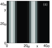
(a)

(b)

(c)

Figure 1: An overhead view of a layer of grains, showing the center of mass height $z_{cm}$ as a function of horizontal position $\left(x,y\right)$ in a cell with horizontal dimensions $L_{x}\times L_{y}=42\sigma\times 42\sigma$, from continuum simulations (a) without noise and (b) with noise. Peaks of the layer corresponding to large center of mass height $z_{cm}$ are shown in white; valleys corresponding to low $z_{cm}$ are shown in black.

In both cases, two wavelengths fit in the box for this box size and frequency (Fig.  1), although simulations without noise show sharper peaks and valleys with larger amplitude than simulations with noise. To compare these amplitudes, I examine the deviation of the height of the center of mass of the layer as a function of horizontal location in the cell from the center of mass height averaged over the entire cell:

$$\psi(x,y,t)=z_{cm}(x,y,t)-\left<z_{cm}(x,y,t)\right>,$$ (1)

where brackets represent an average over all horizontal locations in the cell at a given time $t$. Thus, $\left<\psi^{2}(t)\right>$ represents the mean square deviation of the height of the layer from the mean height of the layer. Note that $\left<\psi^{2}\right>$ is large for layers with high amplitude peaks and valleys, and goes to zero as the layer becomes perfectly flat.

To distinguish between ordered patterns (stripes) and disordered fluctuations, I characterize the long range order of the pattern. I first calculate the power spectrum of the pattern $S\left(k_{x},k_{y},t\right)$ as a function of wavenumbers $k_{x}$ and $k_{y}$. Transforming to polar coordinates $k_{r}$ and $k_{\theta}$ in $k$ space and integrating radially yields the angular orientation of the power spectrum $S(k_{\theta})$. I bin $k_{\theta}$ into 21 bins between $k_{\theta}=0$ and $k_{\theta}=\pi$, and characterize the long range order by the fraction of the total integrated power that lies in the bin with the maximum power:

$$P_{max}=\frac{S_{max}}{\int_{0}^{\pi}S\left(k_{\theta}\right)dk_{\theta}},$$ (2)

where $S_{max}$ is the integrated power within an angle $\pi/21$ of the maximum value of $S(k_{\theta})$. For a perfectly disordered state, with equal power in all directions, $P_{max}$ would approach $\frac{1}{21}\approx 0.05$, while $P_{max}=1$ for a state with all power in a single bin. Thus $P_{max}$ provides a measure of order when stripes form.

I examine $\left<\psi^{2}\right>$ and $P_{max}$ for simulations with varying $\Gamma$. In each case, the simulation begins with a flat layer above the plate with small amplitude initial random fluctuations. The simulation runs for 400 cycles of the plate to reach a periodic steady state. Then $\left<\psi^{2}\right>$ and $P_{max}$ are averaged over the next 50 cycles. Compared to simulations without noise, simulations with noise show greater variation between cycles in their final state; I run these simulations three times for each $\Gamma$ to find an average less influenced by transient behavior. As patterns occur for $\Gamma=2.20$, but not for $\Gamma=1.90$, three additional simulations (for a total of six) were run for each $\Gamma$ in the range $1.90\leq\Gamma\leq 2.20$ to more precisely locate pattern onset.

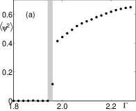
(a)

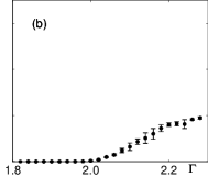
(b)

Figure 2: The mean square deviation $\left<\psi^{2}\right>$ of the local center of mass height from the average center of mass height of the layer as a function of accelerational amplitude $\Gamma$ for simulations without noise (a), and with noise (b). In (a), $\left<\psi^{2}\right>$ is averaged over 50 cycles of a single simulation for each $\Gamma$ (dots). The shaded region $1.94\leq\Gamma\leq 1.96$ indicates the transition between flat layers and layers with non-negligible peaks and valleys. For simulations with fluctuations, the data in (b) are averages (dots) with root mean square deviation (bars) from 50 cycles from each of six trials within the range $1.90\leq\Gamma\leq 2.20$, and each of three trials outside that range.

For simulations without noise, fluctuations in the initial condition decay over time for $\Gamma\lesssim 1.94$, producing a flat layer (Fig. 2a). As $\Gamma$ increases, there is a jump to a periodic state of non-negligible $\left<\psi^{2}\right>$ for $\Gamma=1.96$, and large amplitude waves occur for all $\Gamma>1.96$ (the region $1.94\leq\Gamma\leq 1.96$ is shaded in Fig. 2a). When noise is added, the layer remains flat for some values $\Gamma>1.96$ (Fig. 2b). Non-negligible amplitudes of $\left<\psi^{2}\right>$ occur for $\Gamma\gtrsim 2.0$, but there is not a sharp jump in amplitude.

Since $\left<\psi^{2}\right>$ in Fig. 2b increases gradually with increasing $\Gamma$ rather than showing a sharp onset of waves, I examine the order parameter $P_{max}$ to distinguish between stripes and disordered fluctuations as shown in Fig. 3. For simulations without noise, all layers with $\Gamma\gtrsim 1.96$ show a nearly constant value of $P_{max}\approx 0.4$ (Fig. 3a), corresponding to the stripe patterns seen in Fig. 1a. For $\Gamma\lesssim 1.94$, the initial fluctuations decrease over time, leading to a very flat layer (cf Fig. 2a) with lower $P_{max}$. I identify the critical value $\Gamma_{C}^{cont}=1.95\pm 0.01$ above which stripe patterns are formed in simulations without noise.

For noisy simulations, there is relatively large uncertainty in $P_{max}$ in the shaded region $2.07\lesssim\Gamma\lesssim 2.17$ (Fig. 3b). Visual inspection shows transient behavior in this region, with temporary order appearing and then disappearing, yielding variation in $P_{max}$ from simulation to simulation. Above this shaded region, $P_{max}\approx 0.4$ with low variation, indicating consistently reproducible stripes. Below this region, $P_{max}$ is consistently lower, indicating disordered fluctuations. I thus identify the critical value above which stripe patterns form in simulations with FHD terms $\Gamma_{C}^{FHD}=2.12\pm 0.05$.

These results for continuum simulations without noise $\Gamma_{C}^{cont}=1.95\pm 0.01$ agree with previous continuum simulations showing an abrupt transition from a flat layer to stripe patterns at $\Gamma_{C}^{cont}=1.955\pm 0.005$ Bougie et al. (2005). Simulations with FHD noise, however, show a gradual increase of disordered fluctuations below the onset of ordered stripes, and a transition to stripes at $\Gamma_{C}^{FHD}=2.12\pm 0.05$. While continuum simulations with noise differ from those without noise, they are consistent with previous MD simulations showing the transition to stripe patterns at $\Gamma_{C}^{MD}=2.15\pm 0.01$, with a gradual increase in amplitude of disordered fluctuations below this value Bougie et al. (2005).

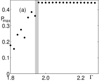
(a)

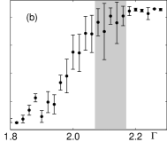
(b)

Figure 3: Global ordering $P_{max}$ as a function of nondimensional accelerational amplitude $\Gamma$ for continuum simulations without noise (a), and with noise (b). For simulations without noise, $P_{max}$ is averaged over 50 cycles from a single simulation and represented as dots, while for simulations with noise, $P_{max}$ is averaged (dots) over multiple simulations, with error bars calculated as root mean square deviation from this average. In both cases, there is a transition (shown in gray) to an approximately constant $P_{max}\approx 0.4$. The transition area shown in gray is $1.94\leq\Gamma\leq 1.96$ in (a) and $2.07\leq\Gamma\leq 2.17$ in (b).

Finally, I investigate the wavelengths of these patterns. Experiments have shown that wavelength $\lambda$ depends on the frequency of oscillation Melo and Douady (1993); Umbanhowar and Swinney (2000). For a range of layer depths and oscillation frequencies, experimental data for frictional particles near pattern onset were fit by the function $\lambda^{*}=1.0+1.1f^{*-1.32\pm 0.03}$, where $\lambda^{*}=\lambda/H$ Umbanhowar and Swinney (2000).

I investigate frequency dependence by holding dimensionless accelerational amplitude $\Gamma=2.2$ constant, while varying dimensionless frequency $f^{*}$. Simulations were conducted in a box of size $L_{x}=168\sigma$, $L_{y}=10\sigma$, and $L_{z}=160\sigma$. This orientation causes stripes to form parallel to the $y-$ axis. The dominant wavelength was calculated from the wavenumber $k_{x}$ in the $x-$ direction which exhibited the maximum power during 50 cycles of the oscillatory state. Due to the periodic boundary conditions and finite box size, wavelengths must fit in the box an integer number of times, yielding uncertainty in the wavelength that would be selected in an infinite box.

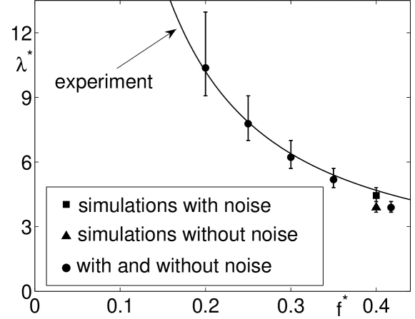
Figure 4: Dispersion relations for stripes which form perpendicular to the long dimension of cells with horizontal dimensions $168\sigma\times 10\sigma$. Data for simulations with noise are shown as squares, without noise as triangles, and points where the two simulations yield the same wavelength are shown as circles. Error bars are calculated exclusively from discretization due to periodic boundary conditions in a finite size box. In both simulations, the dominant wavelength of the final oscillatory state $\lambda$ fits very well to the dispersion relation found in experiments $\lambda^{*}=1.0+1.1f^{-1.32\pm 0.03}$ (solid line) Umbanhowar and Swinney (2000).

For this box size, frictionless MD simulations and continuum simulations without noise have been shown to agree with experimental results for frictional particles through the range $0.20\lesssim ft\lesssim 0.45$; friction appears unimportant in wavelength selection through this range Bougie et al. (2005). Wavelengths found in continuum simulations with and without noise are compared to the dispersion relation fit to experimental data in Fig. 4. Both simulations agree quite well with the experimental fit throughout this range. The addition of noisy fluctuations does not appear to significantly affect the wavelength of the patterns.

In conclusion, continuum simulations without friction can describe important aspects of pattern formation in granular media. With or without noise, frictionless continuum simulations produce patterns with wavelengths consistent with experimental results in layers of particles with friction. For the shaken layers studied in this report, patterns in continuum simulations without noise occur for critical accelerational amplitude $\Gamma_{C}$ approximately 10% lower than in experimentally verified molecular dynamics simulations. Including fluctuating hydrodynamics (FHD) alters the onset of patterns; $\Gamma_{C}$ for continuum simulations with noise is consistent with MD simulations, but not with continuum simulations lacking this noise. These results indicate that fluctuations play a significant role in this system, and also suggest directions for further research. Simulations including memory effects Brey et al. (2009) or other variations in the FHD model could be compared to test which approximations significantly alter pattern formation. In addition, testing the effects of noise on other granular systems will be important in establishing a general theory of granular hydrodynamics and the role of fluctuations within that theory.

References

- Bocquet et al. (2001) L. Bocquet, W. Losert, D. Schalk, T. C. Lubensky, and J. P. Gollub, Phys. Rev. E 65, 011307 (2001).
- Rericha et al. (2001) E. C. Rericha, C. Bizon, M. D. Shattuck, and H. L. Swinney, Phys. Rev. Lett. 88, 014302 (2001).
- Ramírez et al. (2000) R. Ramírez, D. Risso, R. Soto, and P. Cordero, Phys. Rev. E 62, 2521 (2000).
- Bougie et al. (2005) J. Bougie, J. Kreft, J. B. Swift, and H. L. Swinney, Phys. Rev. E 71, 021301 (2005).
- Dufty (2002) J. W. Dufty, in Challenges in Granular Physics, edited by T. Halsey and A. Mehta (World Scientific, 2002).
- Campbell (1990) C. S. Campbell, Annu. Rev. Fluid Mech. 22, 57 (1990).
- Aranson and Tsimring (2006) I. Aranson and L. Tsimring, Rev. Mod, Phys. 78, 641 (2006).
- Goldshtein and Shapiro (1995) A. Goldshtein and M. Shapiro, J. Fluid Mech. 282, 75 (1995).
- Jenkins and Richman (1985) J. T. Jenkins and M. W. Richman, Arch. Rat. Mech. Anal. 87, 355 (1985).
- Sela and Goldhirsch (1998) N. Sela and I. Goldhirsch, J. Fluid Mech. 361, 41 (1998).
- Knight et al. (1996) J. B. Knight, E. E. Ehrichs, V. Y. Kuperman, J. K. Flint, H. M. Jaeger, and S. R. Nagel, Phys. Rev. E 54, 5726 (1996).
- Brey et al. (2001) J. J. Brey, M. J. Ruiz-Montero, and F. Moreno, Phys. Rev. E 63, 061305 (2001).
- Eshuis et al. (2005) P. Eshuis, K. van der Weele, D. van der Meer, and D. Lohse, Phys. Rev. Lett. 95, 258001 (2005).
- Melo et al. (1994) F. Melo, P. Umbanhowar, and H. L. Swinney, Phys. Rev. Lett. 72, 172 (1994).
- Goldshtein et al. (1995) A. Goldshtein, M. Shapiro, L. Moldavsky, and M. Fichman, J. Fluid Mech. 287, 349 (1995).
- Goldman et al. (2003) D. I. Goldman, M. D. Shattuck, S. J. Moon, J. B. Swift, and H. L. Swinney, Phys. Rev. Lett. 90, 104302 (2003).
- Moon et al. (2004) S. J. Moon, J. B. Swift, and H. L. Swinney, Phys. Rev. E 69, 031301 (2004).
- Bizon et al. (1998) C. Bizon, M. D. Shattuck, J. B. Swift, W. D. McCormick, and H. L. Swinney, Phys. Rev. Lett. 80, 57 (1998).
- Bougie et al. (2002) J. Bougie, S. J. Moon, J. B. Swift, and H. L. Swinney, Phys. Rev. E 66, 051301 (2002).
- Landau and Lifshitz (1959) L. D. Landau and E. M. Lifshitz, Fluid Mechanics (Pergamon Books Ltd., Oxford, 1959).
- Zaitsev and Shilomis (1971) V. M. Zaitsev and M. I. Shilomis, Soviet Physics JETP 32, 866 (1971).
- Swift and Hohenberg (1977) J. B. Swift and P. C. Hohenberg, Phys. Rev. A 15, 319 (1977).
- Wu et al. (1995) M. Wu, G. Ahlers, and D. S. Cannell, Phys. Rev. Lett. 75, 1743 (1995).
- Oh and Ahlers (2003) J. Oh and G. Ahlers, Phys. Rev. Lett. 91, 094501 (2003).
- Goldman et al. (2004) D. I. Goldman, J. B. Swift, and H. L. Swinney, Phys. Rev. Lett. 92, 174302 (2004).
- Brey et al. (2009) J. J. Brey, P. Maynar, and M. I. G. García de Soria, Phys. Rev. E. 79, 051305 (2009).
- Bougie (2010) See supplementary material at http://link.aps.org/supplemental/10.1103/PhysRevE.81.032301 for a list of equations used.
- Melo and Douady (1993) F. Melo and S. Douady, Phys. Rev. Lett. 71, 3283 (1993).
- Umbanhowar and Swinney (2000) P. Umbanhowar and H. L. Swinney, Physica A 288, 344 (2000).