Spin current generation and detection by a double quantum dot structure

Abstract

We propose a device acting as a spin valve which is based on a double quantum dot structure with parallel topology. Using the exact analytical solution for the noninteracting case we argue that, at a certain constellation of system parameters and externally applied fields, the electric current through the constriction can become almost fully spin-polarized. We discuss the influence of the coupling asymmetry, finite temperatures and interactions on the efficiency of the device and make predictions for the experimental realization of the effect.

Future progress in the recently very fast developing field of spintronics heavily depends on reliable techniques for the generation and detection of spin-polarized electric currents Wolf et al. (2001). While the majority of proposed devices uses ferromagnetic electrodes of some form, purely semiconductor-based structures possess a number of advantages such as lower power consumption and smaller dimensions as well as better integration options into the conventional circuitry. Probably the best studied elementary structures are quantum point contacts and quantum dots which can, among other things, be used to induce spin currents. Up to now numerous studies have been devoted to the investigation of these possibilities, to name just a few of them: Sergueev et al. (2002); Pustilnik and Borda (2006); Tao et al. (2008). In its simplest form a quantum dot is just an isolated electronic energy level coupled to a number of metallic electrodes by tunneling (and possibly capacitively). The transmission coefficient is then of Lorentzian shape with half-width $\Gamma$ given by the contact transparency between the dot and the electrode. Its resonant behavior immediately suggests one possibility for spin-polarized current generation: the Zeeman-splitting of the level in a finite external field leads to different transmission probabilities for electrons with different spin orientation (the magnetic field is assumed to be finite only on the dot). This method is, however, extremely inefficient since the level-splitting is of the order $0.025$ meV/T for GaAs-based heterostructures and thus even in strong fields significantly smaller than the typical $\Gamma$ ranging between $0.1-10$ meV Goldhaber-Gordon et al. (1998); Cronenwett et al. (1998); Schmid et al. (1998). Generally, the current through the constriction grows with increasing $\Gamma$ such that a compromise must be arranged between the spin polarization quality factor and the current strength. Therefore one has to search for systems which show up transmission properties with even higher degree of nonlinearity than that of a simple (non-interacting) dot. Exactly this situation can be found in double quantum dot systems van der Wiel et al. (2002).

In general a double quantum dot structure even in its simplest incarnation, in which it is modelled by two coupled Anderson impurities, is described by a large number of parameters. The corresponding Hamiltonian is given by Weidenmüller (2003)

$$H=H_{0}+H_{I}+H_{T}\,.$$ (1)

$H_{0}$ is the part describing the two dots ($i=1,2$) via respective fermion annihilators/creators $d_{i,\sigma}^{\dagger},d_{i,\sigma}$ with spin variable $\sigma=\uparrow,\downarrow=\pm$ and two (left/right, $\alpha=L,R$) metallic electrodes. These are modelled by free fermionic continua with field operators $\psi_{\alpha,\sigma}(x)$, which are kept at chemical potentials $\mu_{\alpha}$,

$$H_{0}=\sum_{\alpha,\sigma}H_{\alpha}[\psi_{\alpha,\sigma}]+\sum_{\sigma}\sum_{i=1,2}(E_{i}+\mu_{B}g\sigma h/2)\,d^{\dagger}_{i,\sigma}d_{i,\sigma}\,,$$ (2)

where $E_{i}$ are the bare dot level energies, $\mu_{B}$ is the Bohr’s magneton, $g$ and $h$ are the Landé factor and magnetic field, respectively. Electron exchange between the electrodes and the dots is accomplished by

$$H_{T}=\sum_{i,\alpha,\sigma}\gamma_{i,\alpha}\,d_{i,\sigma}^{\dagger}\psi_{\alpha,\sigma}(0)+\gamma_{\perp}\,d^{\dagger}_{1,\sigma}d_{2,\sigma}+\mbox{H.c.}\,,$$ (3)

where $\gamma_{i,\alpha}$ is the tunneling amplitude between dot $i$ and electrode $\alpha$ and $\gamma_{\perp}$ is responsible for the electron exchange between the dots. The tunnelling is assumed to be local and occur at $x=0$ in the coordinate system of the respective electrode. In general, the tunneling amplitudes are allowed to be complex. Finally, the interactions in the system are taken into account via the last term,

$$H_{I}=\sum_{i}U_{i}\,\,n_{i,\uparrow}\,n_{i,\downarrow}+\sum_{\sigma,\sigma^{\prime}}U_{\perp}n_{1,\sigma}\,n_{2,\sigma^{\prime}}\,.$$ (4)

where $n_{i,\sigma}=d^{\dagger}_{i,\sigma}d_{i,\sigma}$. While $U_{i}$ is responsible for the intradot interaction, $U_{\perp}$ describes the interdot correlation.

In order to illustrate our idea we first neglect the interactions, use $\gamma_{\perp}=0$ and equalize all other tunneling amplitudes to $\gamma$. Transport in such a setup has been investigated in great detail in a number of works, see e. g. Akera (1993); Loss and Sukhorukov (2000); Holleitner et al. (2001); König and Gefen (2002). The fundamental result for the energy-dependent transmission coefficient reads Kubala and König (2002)

$$D_{0}(\omega)=\frac{\Gamma^{2}}{\left[1/(\omega-E_{1})+1/(\omega-E_{2})\right]^{-2}+\Gamma^{2}}\,,$$ (5)

where $\Gamma=2\pi\rho_{0}|\gamma|^{2}$ is the dot-lead contact transparency with dimension of energy. It consists of the tunneling amplitudes and the local density of states $\rho_{0}$ in the leads which is assumed to be very weakly energy-dependent in the relevant range of energies. When the energies of both dots are equal the system is equivalent to the conventional single-site Anderson model as far as the transmission properties are concerned. However, contrary to a single-site quantum dot here perfect reflection is possible when the energy of the incident particles is given by $\omega_{0}=(E_{1}+E_{2})/2$ as soon as $E_{1,2}$ become different. We speculate that this kind of destructive interference is very similar to the one leading to weak localization. Electrons with energy $\omega_{0}$ which travel in the (anti)clockwise direction through the device (and thus on the time-reversal equivalent paths) experience exactly the same phase shift leading to constructive interference at the starting point. The precise form of this kind of antiresonance can be found by rewriting the transmission coefficient (5) in the following form

$$D_{0}(\omega)=\frac{\Gamma}{\sqrt{\Gamma^{2}-E^{2}}}\left(\frac{\Omega_{+}^{2}}{\omega^{2}+\Omega_{+}^{2}}-\frac{\Omega_{-}^{2}}{\omega^{2}+\Omega_{-}^{2}}\right)\,,$$ (6)

where we measure the energy from $\omega_{0}$ and restrict ourselves to $\Gamma>E$, $E=E_{1}=-E_{2}$. Unsurprisingly it is a difference of two Lorentz-shaped curves with the widths $\Omega_{\pm}=\Gamma\pm\sqrt{\Gamma^{2}-E^{2}}$. The antiresonance thus can be made extremely sharp by choosing $E$ very small in comparison to $\Gamma$ by appropriate choice of the gate voltages. In presence of the magnetic field $h$ (we assume that it is not generating any Aharonov-Bohm phase either due to the small area of the dot structure or due to its in-plane orientation) the antiresonance splits in two for electrons with different spin orientation $\sigma$,

$$D_{\sigma}(\omega)=D_{0}(\omega+\sigma h)\,,$$ (7)

where we have redefined $h=\mu_{B}gh/2$ to become the effective energy scale generated by the magnetic field. Thus the transmission coefficients for the electrons with different spin orientations are completely different, see Fig.  1. In fact, the electrons with the energy matching their ‘own’ antiresonance are perfectly reflected while the ones with opposite spin orientation can be made to pass through the structure almost unimpeded.

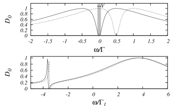
Figure 1: Upper panel: the operation mode of the spin filter. The energy levels are set to $E_{1,2}=\pm 0.5$. The offset $2h=0.5$ is chosen in such a way that the efficiency of the filter reaches its maximum value. All energies are measured in units of $\Gamma$. The shaded area represents a voltage window for the generation of highly spin-polarized current. Lower panel: the effect of asymmetric coupling and inter-dot tunneling. The Fano-lineshape can clearly be identified. Here, the parameters are $E_{1,2}=\pm 1$, $2h=0.15$, $\Gamma_{2}=0.9$ and $\gamma_{\perp}=3.5$. All energies are measured in units of $\Gamma_{1}$. The local maximum of the dotted line coincides with the zero of the solid line to achieve optimal operation of the spin filter.

This is in strong contrast to the single dot structure discussed in the introduction, where perfect transport suppression is difficult to achieve.

Applying finite bias voltage $V$ across the double dot we can in fact generate almost fully spin polarized current as long as $V\ll\Omega_{-}$ and both chemical potentials are symmetrically arranged around the preselected antiresonance, see Fig. 1. In the experimental realization this procedure would amount to a fine-tuning of the dot level energies $E_{1,2}$ as well as of the applied magnetic field. The points where the current is maximally spin-polarized coincide exactly with the points, where the spin-unresolved (conventional) transmission has a dip. Needless to say, in analogy to optical polarizators this effect can also be used for detection of spin-polarized currents.

There are different mechanisms which can destroy the interference and thus significantly affect the quality of spin filtering: (i) finite temperature effects; (ii) the finite interdot tunneling amplitude $\gamma_{\perp}$ as well as the coupling asymmetry; (iii) the effects of intra- as well as interdot interactions. While (i) and (ii) can be (at least in principle) very well controlled in experiments the interactions can be influenced only slightly.

We first analyze the finite-$T$ case. We assume the voltage applied symmetrically around the $\sigma=\uparrow=+$ antiresonance, then the spin-resolved currents are given by

$$I_{\pm} = G_{0}\int d\omega D_{0}(\omega+h_{\pm})$$ (8)

$$\times \left[n_{F}(\omega-V/2)-n_{F}(\omega+V/2)\right]\,,$$

where $n_{F}(\omega)=1/[\exp(\omega/T)+1]$ is the Fermi distribution function, $G_{0}=e^{2}/h$ the conductance quantum per spin orientation and the Zeeman splitting of the dot level energies is taken into account by $h_{+}=0$ and $h_{-}=-2h$ (Without an additional gating of the dot levels by $h$ the antiresonances would, of course, lie at $\pm h$. In order to achieve optimal spin filtering we choose to perform such adjustment of $E_{1,2}$). It is sensible to make predictions for the universal linear response regime first, where the linear conductance $G_{\pm}=I_{\pm}(V)/V$ at $V\rightarrow 0$ is the fundamental quantity. Then for the quality factor of the spin filtering we obtain the following result

$$q=\left|\frac{G_{+}-G_{-}}{G_{+}+G_{-}}\right|\,,$$ (9)

where $G_{\pm}$ is defined by

$$G_{\pm} = \frac{\Gamma}{\sqrt{\Gamma^{2}-E^{2}}}\Biggl{[}\sum_{r,s,t=\pm}\frac{rst\Omega_{r}}{4\pi T}\psi^{\prime}\left(\frac{1}{2}+t\frac{ih_{\pm}+s\Omega_{r}}{2\pi T}\right)$$ (10)

$$+ \sum_{r,s=\pm}\frac{s\left|\Omega_{r}\right|}{4\pi T}\psi^{\prime}\left(\frac{1}{2}-\frac{ish_{\pm}+\left|\Omega_{r}\right|}{2\pi T}\right)\Biggr{]}$$

and $\psi^{\prime}$ is the derivative of the digamma function. As a function of temperature it is plotted in Fig. 2. Well below $T=\Gamma$ very high quality factors are achievable. The effect is more robust for higher values of bare dot energies and applied local field $h$.

Figure 2: Temperature dependence of the quality factor as defined in Eq. (9). Main plot: as a function of the dot energies $E=(0.5,0.75,0.95)=(\text{solid},\text{dotted},\text{dot-dashed})$ for fixed $h=0.5$. Inset: the same for $E=0.95$ and different magnetic fields $h=(0.1,0.25,0.5)$. All energies are measured in units of $\Gamma$.

As far as the asymmetry and $\gamma_{\perp}$ issues are concerned analytical results are possible as well. Interestingly, in both cases the perfect destructive interference is still possible. Hence the spin filter can still be realized as illustrated in the lower panel of of Fig. 1.

The electron-electron interactions on such small quantum dots can usually be quite strong. Despite quite extensive literature the fate of the antiresonance in the case of finite interactions has not yet been addressed. We consider the onsite interactions with amplitudes $U_{1,2}$ first. The transmission coefficient (5) can be found in different ways. One of them is the straightforward calculation of the scattering amplitude of a structure consisting of two Y-shaped junctions arranged in a ring geometry with two in- and outputs between which the two dots are arranged Büttiker et al. (1984); Kubala and König (2003). It is the special property of the dot scattering phases or transmission/reflection amplitudes $r_{\alpha},t_{\alpha}$ as functions of energy $\omega$, which give rise to the antiresonance. In the noninteracting case they are given byKubala and König (2002)

$$r_{\alpha}=\frac{-i\Gamma}{\omega-E_{\alpha}-i\Gamma}\,,\,\,\,\,\,t_{\alpha}=\frac{\omega-E_{\alpha}}{\omega-E_{\alpha}-i\Gamma}\,.$$ (11)

Being plugged into the expression for the full transmission of the structure Büttiker et al. (1984):

$$D_{0}=4\left|\frac{t_{1}t_{2}\bar{r}_{1}-\bar{t}_{1}t_{2}r_{2}-t_{1}t_{2}\bar{r}_{1}+\bar{t}_{1}\bar{t}_{2}r_{2}}{t_{1}t_{2}-\bar{t}_{1}\bar{t}_{2}-\bar{t}_{2}r_{1}-\bar{t}_{1}r_{2}+\bar{t}_{1}\bar{r}_{2}}\right|^{2}$$ (12)

they immediately lead to (5). In fact, (11) are related to the retarded Green’s function (GF) of the individual dots Meir and Wingreen (1992); Yamada (1975a):

$$G^{R}_{\alpha}(\omega)=\frac{1}{\omega-E_{\alpha}+i\Gamma}\,.$$ (13)

On the other hand, the retarded GF (or the transmission matrix) for the case with finite interactions is known to possess the representation Yamada (1975a)

$$G^{R}_{\alpha}(\omega)=\frac{1}{\omega-E_{\alpha}-\mbox{Re}\Sigma^{R}(\omega)+i[\Gamma-\mbox{Im}\Sigma^{R}(\omega)]}\,,$$ (14)

where $\Sigma^{R}(\omega)$ is the self-energy due to the onsite interaction. Because we are only interested in the transmission properties around $\omega=0$ it is sufficient to possess information about the self-energy behavior around this point. A good approximation for the self-energy is the one of the ordinary Anderson impurity model. Luckily, there is a low-energy expansion for this $\Sigma^{R}(\omega)$ due to Yamada (1975b, a); Yosida and Yamada (1975, 1970); Zlatić and Horvatić (1980, 1983). The main message is that the leading order expansion in $\omega$ is provided by the correction to the real part Oguri (2001),

$$\mbox{Re}\Sigma^{R}_{\alpha\sigma}(\omega)=\chi_{c}(E_{\alpha}+U/2)+\sigma h\chi_{s}$$

$$+\left(1-\frac{\chi_{c}-\chi_{s}}{2}\right)\,\omega+\dots\,,$$ (15)

where $\chi_{c,s}$ are the static charge/spin susceptibilities and are known for arbitrary $U$ from the Bethe ansatz calculations Zlatić and Horvatić (1983). $(E_{\alpha}+U/2)$ plays the role of the electron-hole symmetry breaking field. Thus we conclude that up to the finite shift $\delta E_{\alpha}=\mbox{Re}\Sigma^{R}_{\alpha\sigma}(0)$ the antiresonance survives and we expect the same quality of spin filtering is achievable. The next question about the antiresonance width can only be answered with the next order expansion in $\omega$ at hand. Since the leading order for the imaginary part of the self-energy is $\omega^{2}$ (which is not surprising since it is responsible for the dissipative part and thus for inelastic processes) the form of the antiresonance is dominated by the second term of (Spin current generation and detection by a double quantum dot structure). Then the transmission is given by

$$D_{0}=\frac{\Gamma^{2}}{\Gamma^{2}+\left(\frac{1}{\omega\frac{\chi_{1c}-\chi_{1s}}{2}-\left(E_{1}+\delta E_{1}\right)}+\frac{1}{\omega\frac{\chi_{2c}-\chi_{2s}}{2}-\left(E_{2}+\delta E_{2}\right)}\right)^{-2}}\,.$$

In case of a small-$U$ expansion Zlatić and Horvatić (1980) one can rewrite this again as a sum of two Lorentzians. Apart from a rescaling of the $\Omega_{\pm}\rightarrow\Omega_{\pm}/\alpha$ where $\alpha=\frac{U^{2}}{2\pi^{2}}\left(3-\frac{\pi^{2}}{4}+\left(\frac{25}{3}-\frac{3\pi^{2}}{4}\right)\frac{E^{2}}{\Gamma^{3}}\right)$ one finds equation (6). The effects of higher order terms of $\omega$ can be understood using the $U$-expansion results of Zlatić and Horvatić (1980). To illustrate their influence on the transmission we plotted the antiresonance upon inclusion of the $\omega^{2}$ terms in Fig. 3. The effect of interactions on the quality factor of spin filtering is presented in Fig. 4.

Interactions between electrons on different dots are often weak in comparison to $U_{1,2}$. Thus we can treat them perturbatively. It is a tedious but straightforward calculation so we suppress the details. Already in the lowest order the correction to the transmission coefficient reveals an interesting effect of antiresonance enhancement, see Fig. 5. While the intradot interactions appear to narrow the antiresonance the effect of the interdot interactions is quite the opposite.

Figure 3: Influence of weak interactions on the effective tranmission coefficient around the antiresonance. Main plot: antiresonance with self-energy correction up to linear order in $\omega$ and second order in $U/\pi$. The energy levels of the dots are $E=0.5$. Inset illustrates the effect of second order corrections in $\omega$ and $U/\pi$. Again, the dot energies are $E=0.5$ and the intra-dot interaction is $U=1$. Energies are measured in units of $\Gamma$.

Figure 4: Temperature dependence of the quality factor in the interacting case for $E=0.95$ and $h=0.5$ and different interaction strengths. Energies are measured in units of $\Gamma$.

As we have shown above the perfect antiresonance is not destroyed by the not too strong Coulomb interactions within the device. However, we expect that this is not the case as soon as interactions with the environment are included. These effects can be discussed by modifying the respective dot Green’s function (14) or using the appropriate self-energy. It is not only possible to analyze perturbations with particle exchange with the environment (leakage currents etc.) but also to include interactions with phonon baths and electromagnetic environments.

Figure 5: Effect of inter-dot interactions on the transmission coefficient around the antiresonance for different values of the interaction strength. The energy levels of the dot are given by $E=0.5\Gamma$. All energies are measured in units of $\Gamma$.

To conclude, we propose a device for spin-polarized current generation and detection. It is based on the double quantum dot structure and operates around the antiresonance in transmission achieved at certain constellation of dot parameters and external fields. We discuss the quality factor of spin filtering as well as its robustness against intrinsic and extrinsic factors such as finite temperature, interaction effects and contact to the environment. We expect that the discussed spin-filtering techniques can be implemented in the up-to-date double quantum dot devices such as those presented in Holleitner et al. (2001); Wilhelm et al. (2002).