New efficient methods to calculate watersheds

Abstract

We present an advanced algorithm for the determination of watershed lines on Digital Elevation Models (DEMs), which is based on the iterative application of Invasion Percolation (IIP) . The main advantage of our method over previosly proposed ones is that it has a sub-linear time-complexity. This enables us to process systems comprised of up to $10^{8}$ sites in a few cpu seconds. Using our algorithm we are able to demonstrate, convincingly and with high accuracy, the fractal character of watershed lines.

We find the fractal dimension of watersheds to be $D_{f}=1.211\pm 0.001$ for artificial landscapes, $D_{f}=1.10\pm 0.01$ for the Alpes and $D_{f}=1.11\pm 0.01$ for the Himalaya.

1 Introduction

The concept of watershed arises naturally in the field of Geomorphology, where it plays a fundamental role in e.g. water management [1, 2, 3], landslide [4, 5, 6, 7] and flood prevention [6, 8, 9]. Moreover, important applications can also be found in seemingly unrelated areas such as Image Processing [10, 11, 12] and Medicine [13, 14, 15, 16, 17]. Watersheds divide adjacent water systems going into different seas and have been used since ancient times to delimit boundaries. Border disputes between countries, like for example the case of Argentina and Chile [18], have shown that it is important to fully understand the subtle geometrical properties of watersheds. Geographers and geomorphologists have studied watersheds extensively in the past. There have also been preliminary claims about fractality [19] but they were restricted to small-scale observations and therefore inconclusive. Despite the far reaching consequences of scaling properties on the hydrological and political issues connected to watersheds no detailed numerical or theoretical study has yet been performed.

In particular in image processing or computer vision the interest in development of efficient algorithms is high. There one tries to simplify and/or change an images representation such that it is more meaningful or easier to analyze. This is done by image segmentation, e.g. partitioning a digital image into multiple segments (sets of pixels, also known as superpixels). Typically one locates like this objects and boundaries (lines, curves, etc.) in images. More precisely, image segmentation is the process of assigning a label to every pixel in an image such that pixels with the same label share certain visual characteristics as color, intensity or texture. Adjacent segments are significantly different with respect to the same characteristic(s) [12]. This sounds familiar and, although many other methods, such as clustering, histograms [20], edge-detection [21], region growing [10], level-set or graph partitioning [22], have been developed for that purpose, also watersheds are currently used. This because, if one transforms an image to its color gradient representation and calculates the watersheds on the so achieved DEM like data, one can identify the obtained catchment basins as the different (color) regions and their boundaries to be represented by the watersheds.

It is the purpose of the present paper to present an advanced method, which allows us to study the geometrical properties of watersheds on huge landscapes and with high statistics. Applied to an artificial landscape model we show results on length scales spanning over three orders of magnitude yielding highly accurate estimates of the fractal dimension of watersheds. Our algorithm is based on an iterative invasion-percolation (IP) like model. We compare to other algorithms in use and show the advances of our method. Furthermore, we prove the equivalence of our IP-based method to the so called flooding algorithm. Finally the method is applied to Digital Elevation Maps (DEM) from regions including the Alps and the Himalayas.

2 The two methods

Traditional cartographical methods for basin delineation relied on manual estimation from iso-elevation lines and required a good deal of guess work. Modern procedures are based upon the automatic processing of DEM or Grayscale Digital Images where gray intensity is transformed into height. One of the most popular algorithms for watershed determination [10] (compare also flooding later) uses rather complicated data structures and at least one pass over all pixels in order to calculate watersheds, and is adequate for grayscale images, i.e. integer-height spaces. In the following, we will present a much more efficient technique.

Let us consider a DEM with sites $i$ having heights $h_{i}$. We define the set of sites $S_{k}$, $k=0,1,\ldots,N_{sinks}$, to be the sinks of our system. On natural landscapes these sinks are the natural water-outlets of the terrain, as for example a lake, a river or an ocean. We consider that at each time step, water flows to the lowest-lying site on the perimeter of a flooded region. If when starting from $i$, sink $S_{k}$ is flooded before any other, then site $i$ and the whole flooded region are considered to belong to the catchment basin of sink $S_{k}$, equivalently one says that $i$ drains to $S_{k}$. This procedure introduces a classification of lattice sites, i.e. a subdivision into non-overlapping subsets whose union is the entire lattice. The sets of bonds separating neighboring basins we call watersheds. We are interested in the geometrical properties of a single watershed line. But as natural landscapes normally contain more than one sink and hence more than one single line, it is difficult to study long range properties. We therefore restrict ourselves to study two-sink systems, or in other words studying only the main watershed with respect to these two sinks. Although we use these restrictions, our algorithm, which we will describe in the following, is able to deal also with multiple-sink systems. This because it is not restricted to certain number of sinks/labels but is free to deal with as many as one would like to.

In our algorithm, that we call IP-based algorithm, a cluster is started from site $i$ and grown by adding, similar to Invasion Percolation (IP), at each step, the smallest-height site on its perimeter until the first sink is reached (see figure 1). This can be done rather quickly when using binary heaps or other tree methods to sort the list of perimeter sites according to their height values. This procedure is related to Prim’s algorithm for growing Minimum Spanning Trees (MST) from $i$ [24, 25]. When implemented blindly over the whole lattice, however, this process would be inefficient since in principle a new cluster has to be grown from each site $i$. By noting that all sites occupied by a cluster at the time the sink is reached also drain to that sink, it becomes clear that we can set for each site in the cluster a link to that sink. This leads to two improvements, first, we do not need to treat again the sites contained in the cluster as we can directly link them to the sink reached by the cluster, and second, we can stop growing clusters already when we reach a site which has an existing link to a sink. Like this, the algorithm has to visit each site only once. But still each site on the map has to be visited. Let us assume we already know a line dividing the system and we want to check if this line is really the watershed of the current system. To prove this we actually only need to test the sites adjacent to the watershed line if they belong to different sinks on the two sides of the line. Hence the subset of the system, formed by these adjacent sites, is the minimal subset we have to test, meaning to grow IP-clusters from them, in order to clearly determine the watershed. Unfortunately we do not know in advance the exact form or position of the watershed, neither we know any of the sites in that minimal subset. The only thing we know is, that the watershed is located somewhere in between the two sinks. This means that, whatever path we follow, to go from one sink to the other, we have to cross the watershed. The sites we visited on such a path, before the watershed traversal, belong to the sink we started from and the sites afterwards belong to the second sink. This is what we now can use to find the first two sites of the minimal subset. We follow a straight line of sites connecting the two sinks. Starting from one sink we follow the connection site by site and grow IP-clusters from these sites. We proceed until we reach the first site that drains to the second sink, which means that we have crossed the watershed (see figure 1). The bond between the last two sites, that drain to different sinks, is part of the watershed line and the two sites belong to the minimal subset as mentioned above. Now we can reconstruct the minimal subset and the set of bonds forming the watershed line by just following step by step the direction of the already found watershed at one of its two ends and testing the next two sites to find if the direction changes by $\pm 90$ degrees or remains the same. We just walk along the watershed and hence have only to test slightly more sites than in the minimal subset (see figure 1). Of course the IP-clusters for these sites have to be grown until they reach a sink or sink-connected site, but there are typically large parts of the terrain that need not be visited at all by the algorithm in order to determine the entire divide. For use in multiple sink systems one would only have to consider additionally branching and joining of the watershed lines (also only one starting bond has to be found).That only a part of the system has to be considered (compare figure 2) and there each site only once, is probably the biggest advantage of this procedure. The described algorithm is fast enough to allow for the determination of watersheds on lattices comprising $10^{8}$ sites, in a few CPU seconds on a normal workstation.

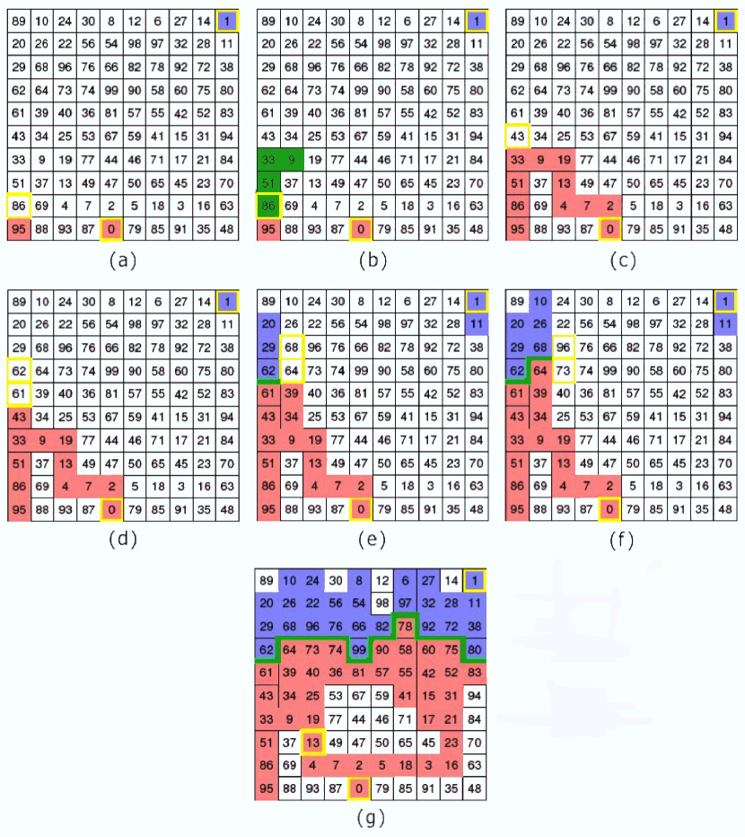
Figure 1: Different stages during the search for the main watershed (green lines), red/blue for the labels to the two sinks, green are visited but not yet labeled sites, the numbers mark the integer heights of the corresponding site and the yellow box surrounds the starting site of the current IP-cluster, right and left periodic boundary conditions are applied. Upper most and lower most bonds connect to the sinks (which are entire rows). Further the lowest two sites are already labeled. (a)-(c) shows the growth of an IP-cluster until reaching a sink. (a)-(e) search for the first watershed bond, growing IP-clusters of each site along the first column consecutively. (e)-(g) Following the watershed.

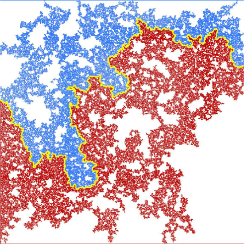
Figure 2: Labels of the sites for a random landscape obtained during the run of the IP-based algorithm. Red labels (lower part) belong to the sink at the bottom row and the blue ones (upper part) to the sink at the upper most row. The watershed is marked in yellow. Only the colored sites are visited by the algorithm, meaning that white sites have not to be considered by the algorithm in order to obtain the right set of watershed bonds.

In the following we describe a slightly adjusted version of the commonly used watershed algorithm for image segmentation ([10]) in order to compare efficiency and prove equivalency to our IP-based algorithm (actually it is making use of disjoint-set data structures). In this procedure, which we call flooding, the whole lattice is flooded (or occupied) in order of increasing height, i.e. at time $t$ all sites with $h_{i}<h(t)$ are occupied and $h(t)$ grows site per site in time. This procedure is also related to Kruskal’s algorithm for growing MST’s [24, 25]. It is assumed that each site has a height, which is a real number, such that after sorting them, a unique sequence of sites is defined. At the beginning, each sink is assigned a different label, and we will furthermore specify that a cluster of occupied sites that gets connected (through a path of occupied sites) with a sink is labelled accordingly, i.e. labels propagate from the sinks. Clusters of occupied sites not yet in contact with any sink remain unlabeled. Whenever two different labels would get in contact with each other because of the addition of a new site, the (unique) bridging site is first labelled with the label of its lowest-lying neighbor. Next all bonds connecting sites with different labels are “cut” so that labels from different sinks never mix. Bonds connecting different labels are called bridges. When this flooding procedure is completed, the different labels identify the corresponding catchment basins and the set of bridges, i.e. the set of bonds separating the different basins, identifies the watershed(s). In the described form the sinks are predefined by hand or applying some criteria. Of course one can reformulate this procedure to identify all intrinsic catchment basins automatically by just introducing new labels when a site gets occupied that has only non-occupied neighbors. This will in fact return all possible watersheds on the current landscape, even of the smallest basins, which is probably not what one would like to have. Unfortunately using the above described flooding algorithm one has in general to consider each site or pixel to completely determine the watershed, such that, already without considering the needed sorting, this algorithm performs less efficient than the presented IP-based algorithm.

3 Equivalence of Methods

We now sketch a simple proof for the equivalence of these two procedures. During the flooding growth a set of unlabeled sites that become labelled by occupying site $b$ is called a lake and $b$ is called its outlet. The height of all sites in a lake is bounded by that of its outlet, i.e. $h(i)\leq h(b(i))$. Let us stop the flood procedure when site $i$ gets labelled for the first time, say with label $S_{k}$. Now start an IP cluster from $i$ and let it grow for as long as it takes until some sink is first occupied. During the growth of this cluster, which proceeds by always adding the lowest-lying site on the perimeter, several lakes and their outlets may be occupied. We need to demonstrate that no bridge will be ever traversed during this IP growth, and therefore that sink $S_{k}$ will be occupied first. During the growth of the IP cluster, a lake will be entirely flooded i.e. the water will reach the level of its outlet. Since all bridges by definition are higher than the outlet of a lake (because by definition bridges were occupied later than the outlet), clearly the next occupation will proceed through the outlet and not through the bridge. Therefore no bridge will be ever traversed thus proving the equivalence of both procedures.

It is important to note that, although conceptually equivalent, the IP and the flooding algorithms are markedly different in terms of computational performance. First, the flooding needs a sorting of the sites according to their heights, which needs at least $O(N)$ time. Additionally it has been shown by Fredman and Saks in [23] that building the disjoint-set data structure, which the algorithm is based on, needs in all cases at least $O(\alpha(N)N)$, where $\alpha(N)$ is the inverse Ackermann function, which is constant for almost all values of $N$. Hence the flooding scales at least with $O(N)$. In figure 3, for the random artificial landscape case, the number of sites visited by the IP-based algorithm is shown together with its scaling in linear dimension $L$, which clearly points out the sub-linear time-complexity of this method. The total number of visited sites $N$ scales as $N\sim L^{D_{f}}$ with $D_{f}=1.8\pm 0.01$. This is comparable to what is found in nature. There, river networks show fractal dimensions between $1.7$ and $1.9$ [26, 27, 28, 29, 30, 31]. On large scales we expect this fractal dimension to be dominated by the largest IP-cluster we grow, for which we found a fractal dimension that is in good agreement with literature and the result for the total number of visited sites. Furthermore we expect that the algorithm is even more efficient on natural landscapes, as the largest IP-cluster will most probably follow the main stream. Hence scaling like the main stream, which is reported to have fractal dimensions between $1.0$ and $1.2$ [26, 27, 28, 29, 30, 31].

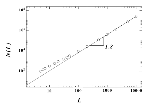
Figure 3: Log-log plot of the number $N(L)$ of sites visited by the IP-based algorithm, in order to determine the watersheds on artificial landscapes, as a function of linear dimension $L$ (circles). Solid line shows the least squares fit to the five last data points, which gives a dimension $D_{f}=1.8\pm 0.01$ for large scales ($N\sim L^{D_{f}}$).

4 Results

As an example we applied the IP-based algorithm to artificial landscapes., where the height of each site on the lattice is an independent random variable uniformly distributed between 0 and 1 , and two sinks are defined respectively as the upper- and lowermost lines of the lattice. Due to the high efficiency of the method we could process a huge amount of data and hence gather a lot of statistics. This enables us to very precisely estimate the fractal dimension of the watershed using the mass-scaling. We measured the total length of the resulting watersheds and averaged this value over at least $10^{4}$ samples for a given lattice size. The results for artificial landscapes are shown in figure 4. Our data is strikingly straight on a log-log plot, which warrants neglecting finite size corrections. Hence, the fractal dimension is measured as the least squares fit to the slope of the shown data. We find that the watershed is a fractal, i.e. $M\sim L^{D_{f}}$, with a fractal dimension $D_{f}=1.211\pm 0.001$ . This value of $D_{f}$ is close to that found for Disordered Polymers ($\approx 1.2$ [32]), “strands” in Invasion Percolation ($1.22\pm 0.01$ [33]), and paths on MST’s ($1.22\pm 0.01$ [24]). The roughness exponent found for the watersheds is equal to unity within the statistical error bars, supporting the fact that they are indeed self-similar fractal objects and not self-affine.

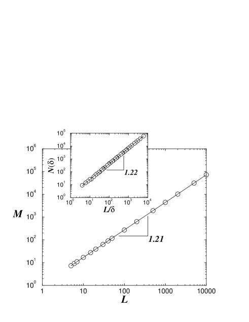
Figure 4: The mass $M$ of the watershed of (uncorrelated) random-height maps scales with linear dimension as $M\sim L^{D_{f}}$, with $D_{f}=1.211\pm 0.001$. A box-counting procedure (inset) gives a consistent result. This fractal dimension is independent of the type of disorder, as long as each height is an uncorrelated random variable.

We also applied the IP algorithm to study the fractal properties of watersheds on naturally occurring landscapes, which clearly have long range correlations [34]. Of course, if we would like to estimate the fractal dimension of a single watershed line of one given landscape, as is the case for these natural topographies, we cannot work with the statistic approach used above for the artificial ones. Therefore we have to choose another method. As we follow the watershed bond per bond and hence have the correct ordered set of bonds, we can easily apply a yard stick method. Measuring now the length of the watershed in terms of a given yard stick size, meaning measuring the length on a certain resolution, we can define the corresponding fractal dimension again. We checked this procedure also on several realizations of artificial landscapes and found the newly estimated fractal dimension to agree with the above presented $D_{f}=1.211\pm 0.001$ within the error bars. Therefore we can assume that this equality is also true for natural landscapes. Now, using topographic data derived from the Shuttle Radar Topography Mission (SRTM) [35], we analyzed several mountainous regions and determined their watersheds within the available resolution of 3 arc-sec (i.e. roughly $90~{}m$). As shown in figure 5, a yard-stick analysis of the watershed performed in the range $100~{}m<L<200~{}km$ for the Alps and Himalayas gives fractal dimensions that are indistinguishable within their error bars, namely $D_{f}^{Al}=1.10\pm 0.01$ and $D_{f}^{Hi}=1.11\pm 0.01$, respectively. The error bars were obtained by determining the lines of maximal and of minimal slope that would still be consistent with the data in figure 5. Again the roughness exponent found for the watersheds is equal to unity within the statistical error bars, hence we have still self-similar fractal objects and not self-affine for intermediate to large scales. The origin of the upper and lower-size scales is clear. On large scales ($>200~{}km$) the watershed follows the direction of the main crust foldings, which depends on processes occurring on the scale of tectonic plates, which are non-fractal. Hence the scaling should be essentially linear ($D_{f}=1$). Although beyond our resolution, at small scales ($<100~{}m$), below the size of an individual mountain, the watershed would connect peaks and troughs, which are typically self-affine.

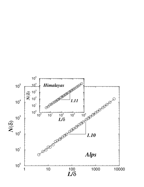
Figure 5: Log-log plot showing the box-counting results for the Alps watershed. The solid line is the best fit to the data which gives a fractal dimension of $D_{f}^{Al}=1.10\pm 0.01$. The inset shows our results for the watershed calculated on the Himalayas. The fractal dimension in this case is $D_{f}^{Hi}=1.11\pm 0.01$.

It is important to notice that the fractal dimension of the watershed line $D_{f}$ is by definition independent of the type of disorder on the landscape, as long as each height is an uncorrelated random variable because only the spatial order of the random variables (heights) in the system matters and not their relative numerical differences. The small discrepancies (around $10\%$) between fractal dimensions of watersheds in the natural topographical data taken from SRTM and the artificial random landscapes can be explained by the presence of correlations in the first case. In particular, long-range correlations in space have been reported in a large variety of physical, biological and geological systems [36, 37, 38, 39, 40].

5 Conclusions

We presented an advanced numerical algorithm of sub-linear time-complexity and showed its equivalence to a currently used watershed algorithm. Giving some qualitative arguments and analysis we pointed out the improved efficiency of the presented method. We further investigated the watershed topology of natural and synthetic DEM’s. Our results show that watersheds generated on very large ($10^{8}$ sites) uncorrelated random landscapes are self-similar with fractal dimension $D_{f}=1.211\pm 0.001$. Natural watersheds calculated from landscapes of mountainous regions like the Alps and Himalayas also display self-similarity, but with slightly smaller fractal dimensions, $D_{f}^{Al}=1.10\pm 0.01$ and $D_{f}^{Hi}=1.11\pm 0.01$, respectively. The difference between the fractal dimensions arises probably due to the fact that long-range correlations exist in the natural system. The fractality of watersheds has widespread consequences on its susceptibility to perturbations of the topology and transport properties at the boundary of catchment basins. These are questions that will be investigated in the future.

References

- [1] Vorosmarty C J, Federer C A and Schloss A L, Evaporation functions compared on US watersheds: Possible implications for global-scale water balance and terrestrial ecosystem modeling., 1998 J. Hydrol. 207 147
- [2] A. Y. Kwarteng et al., Formation of fresh ground-water lenses in northern Kuwait, 2000 J. Arid Environ. 46 137
- [3] Sarangi A and Bhattacharya A K, Comparison of Artificial Neural Network and regression models for sediment loss prediction from Banha watershed in India, 2005 Agr. Water Manage. 78, 195
- [4] Dhakal A S and Sidle R C, Distributed simulations of landslides for different rainfall conditions, 2004 Hydrol. Process.a 18 757
- [5] Pradhan B, Singh R P and Buchroithner M F, Estimation of stress and its use in evaluation of landslide prone regions using remote sensing data, 2006 Adv. Space Res. 37 698
- [6] Lee K T and Lin Y T, Flow analysis of landslide dammed lake watersheds: A case study, 2006 J. Am. Water Resour. As. 42 1615
- [7] Lazzari M et al., Natural hazards vs human impact: an integrated methodological approach in geomorphological risk assessment on the Tursi historical site, Southern Italy, 2006 Landslides 3 275
- [8] Burlando P, Mancini M and Rosso R, FLORA - A distributed Flood Risk Analyzer, 1994 IFIP Trans. B 16 91
- [9] Yang D Q et al., Streamflow response to seasonal snow cover mass changes over large Siberian watersheds, 2007 J. Geophys. Res.-Earth 112 F02S22
- [10] Vincent L and Soille P, Watersheds in digital spaces - an efficient algorithm based on immersion simulations, 1991 IEEE T. Pattern. Anal. 13 583
- [11] Gao H, Siu W C and Hou C H, Improved techniques for automatic image segmentation, 2001 IEEE T. Circ. Syst. Vid. 11 1273
- [12] L. G. Shapiro, and G. C. Stockman, Computer Vision, 2001 New Jersey: Prentice-Hall 279-325
- [13] Bruyant P P and King M A, The Rain Algorithm: An edge-preserving smoothing filter using the watershed transform, 2002 J. Nucl. Med. 43 206P
- [14] Mao K Z, Zhao P and Tan P H, Supervised learning-based cell image segmentation for P53 immunohisto-chemistry, 2006 IEEE T. Bio.-Med. Eng. 53 1153
- [15] Vidal F P et al., Principles and applications of computer graphics in medicine, 2006 Comput. Graph. Forum 25 113
- [16] Yan J Y et al., Marker-controlled watershed for lymphoma segmentation in sequential CT images, 2006 Med. Phys. 33 2452
- [17] Ikedo Y et al., Development of a fully automatic scheme for detection of masses in whole breast ultrasound images, 2007 Med. Phys. 34 4378
- [18] Reports of International Arbitral Awards, The Cordillera of the Andes Boundary Case (Argentina, Chile) (United Nations Treaty Collection, 2006). Available at http://untreaty.un.org/cod/riaa/cases/vol_IX/29-49.pdf.
- [19] Breyer S P and Snow R S, Drainage-basin perimeters - A fractal significance, 1992 Geomorphology 5 143
- [20] Ohlander R, Price K and Raj Reddy D, Picture Segmentation Using A Recursive Region Splitting Method, 1978 Computer Graphics and Image Processing 8 313-333
- [21] Pathegama M P and Göl Ö, Edge-end Pixel Extraction for Edge-based Image Segmentation, 2005 World Academy of Science, Engineering and Technology 2 164
- [22] Shi J and Malik J, Normalized Cuts and Image Segmentation, 2000 IEEE T. Pattern Anal. 22 888
- [23] Fredman M and Saks M, The cell probe complexity of dynamic data structures, 1989 Proc. of the Twenty-First Ann. ACM Symp. on Theory of Computing 345
- [24] Dobrin R and Duxbury P M, Minimum spanning trees on random networks, 2001 Phys. Rev. Lett. 86 5076
- [25] Barabasi A L, Invasion percolation and global optimization, 1996 Phys. Rev. Lett. 76 3750
- [26] Rodriguez-Iturbe I and Rinaldo A, Fractal River Basins, 1997 Cambridge: Cambridge University Press
- [27] Maritan A, Rinaldo A, Rigon R, Giacometti A, and Rodr guez-Iturbe I, Scaling laws for river networks, 1996 Phys. Rev. E 53 1510 - 1515
- [28] De Bartolo S G, Veltri M and Primavera L, , 2006 Journal of Hydrology 322 181 191
- [29] Horton R E, Drainage basin characteristics, 1932 EOS Trans. AGU 13 350 361
- [30] Hack J T , Studies of longitudinal profiles in Virginia and Maryland, 1957 USGS Professional Papers 294-B 46 97
- [31] Melton M A, Correlation structure of morphometric properties of drainage systems and their controlling agents, 1958 J. of Geology 66 35 56.
- [32] Cieplak M, Maritan A and Banavar J R, Optimal paths and domain-walls in the strong disorder limit, 1994 Phys. Rev. Lett. 72 2320
- [33] Cieplak M, Maritan A and Banavar J R, Invasion percolation and Eden growth: Geometry and universality, 1996 Phys. Rev. Lett. 76 3754
- [34] Turcotte D L, Fractals and Chaos in Geology and Geophysics, 1997 Cambridge: Cambridge University Press, 2nd ed.
- [35] Farr T G et al., The shuttle radar topography mission, 2007 Rev. Geophys. 45 RG2004
- [36] Dynamics of Fractal Surfaces, edited by F. Family and T. Vicsek, 1991 Singapore: World Scientific
- [37] Bunde A and Havlin S, Fractals in Science, 1994 Berlin: Springer-Verlag
- [38] Sahimi M, Non-linear and non-local transport processes in heterogeneous media: from long-range correlated percolation to fracture and materials breakdown, 1998 Phys. Rep. 306 213
- [39] Sapoval B, Baldassarri A and Gabrielli A, Self-stabilized fractality of seacoasts through damped erosion, 2004 Phys. Rev. Lett. 93 098501
- [40] Schorghofer N and Rothman D H, Acausal relations between topographic slope and drainage area, 2002 Geophys. Res. Lett. 29 1633