Variable range hopping in the Coulomb glass

Abstract

We use a mean-field (Hartree-like) approach to study the conductance of a strongly localized electron system in two dimensions. We find a crossover between a regime where Coulomb interactions modify the conductance significantly to a regime where they are negligible. We show that under rather general conditions the conduction obeys a scaling relation which we verify using numerical simulations. The use of a Hartree self-consistent approach gives a clear physical picture, and removes the ambiguity of the use of single-particle tunneling density-of-states (DOS) in the calculation of the conductance. Furthermore, the theory contains interaction-induced correlations between the on site energy of the localized states and distances, as well as finite temperature corrections of the DOS.

I Introduction

The unusual temperature dependence of the conductance of strongly disordered samples has generated a great interest in the past four decades. These systems manifest an interplay between disorder and interactions, which is ubiquitous in nature, and which renders the problem difficult theoretically and rich experimentally efros ; efrosbook2 ; Gantmakherbook ; pollakbook1 . In these disordered systems, conductance occurs via phonon assisted hopping between localized states, whose size is roughly the localization length $\xi$. The measured low-temperature conductance of various disordered samples shows temperature dependence different than simple activation, of the type $\sigma\sim e^{-\left(\frac{T_{0}}{T}\right)^{\zeta}}$, with $\zeta<1$.

Mott’s theory (”Mott’s law”) for Variable Range Hopping (VRH) mott , which ignores the Coulomb interactions, gives $\zeta=\frac{1}{d+1}$ and $T_{0}$ equal to the non-interacting mean level spacing in a localization volume $\delta_{\xi}=1/\nu_{0}\xi^{d}$; with $d=1,2$ or 3 the dimension of the system and $\nu_{0}$ the density-of-states.

As first pointed out by Pollak pollak_ , interactions affect the single-particle tunneling density-of-states (DOS), and thus may possibly influence the conductance. Efros and Shklovskii (ES) efros2 obtained an analytic bound for the so-called Coulomb gap in the DOS, which was later observed experimentally coulomb_gap_experimental ; butko . Using the interaction-modified DOS to find the conductance (treating the problem as essentially non-interacting from this point) one obtains (”ES’s law”) $\zeta=\frac{1}{2}$, in any dimension $d$. In ES’s law $T_{0}$ is given by the Coulomb energy of the localized state $E_{\xi}=e^{2}/\xi$. The Mott and the ES laws, as well as the crossover between the two regimes, were observed in various experiments Mott_ES_experiments . Many qualitative features that this complicated system exhibits can be obtained using rather simple and heuristic arguments. However, using the single-particle DOS in the calculation of the conductance, neglecting finite temperature effects on the DOS and ignoring correlations between energies and spatial locations is not discussed or can not be justified in the framework of the heuristic arguments (see [Pollak_1_over_2, ] for an elaborate discussion).

In this work we study the crossover between Mott’s and ES’s laws, using the theoretical framework of a Hartree theory coulomb_gap_mean_field ; amir_glass . The Hartree theory takes into account interactions in a self-consistent manner. Hence, it gives a well defined procedure for calculating various physical properties and allows us to develop a clear intuitive physical picture. Within the Hartree approximation the use of a renormalized single-particle DOS is built in, with the electrons moving in an effective potential due to the other electrons. While various other theories neglect the interaction-induced correlations between on-site energies and position shegelski ; goedsche , these exist in the theory we present: The mean-field equations amir_glass contain both the electronic site positions and the renormalized energies, and therefore correlations between the two exist in the self-consistent solution. We emphasize that within the Hartree theory the average occupation and renormalized energy are different at each electronic site. Albeit, the Hartree method is uncontrolled as there is no small parameter in the theory. It is therefore difficult to estimate rigorously its limit of validity. Nevertheless, due to the long-range nature of the Coulomb interactions, the potential energy at a given site is renormalized by a large number of electronic sites. This suggests that the approximation should be valid, and we believe it should be applicable for a wide range of system parameters. Indeed, the mean-field picture yields the well-established results for the Coulomb gap in two dimensions amir_glass , and captures well the results of aging experiments unpublished .

In this work we demonstrate, in two dimensions, that the Hartree theory yields the ES’s and Mott’s laws including the crossover between them, for which we derive an analytical scaling relation that holds under generic conditions, extending the results of Refs. ora_VRH ; meir_scaling ; aharony_sarachik ; rosenbaum . This is a proof that interaction-induced correlations between location and energy as well as finite temperature corrections are not essential for determining the conductance.

The Hartree approximation involves a numerical procedure. Nevertheless, it clarifies our physical understanding of the complex Coulomb glass. Its success in reproducing equilibrium (the gap in the DOS) and near equilibrium properties (the conductance) and its simplicity indicate that it may be usable in the estimates of dynamical properties. Indeed, this was done in [unpublished, ].

The structure of the paper is as follows. We first present the model, and the heuristic arguments leading to the Mott and ES laws. We show the Hartree theory gives a Coulomb gap consistent with other theoretical and numerical approaches, and study the temperature dependence of the DOS. We then explain the mean-field approach to determining the conductivity, and the numerical procedure involved. Finally, we analyze the crossover between the two regimes analytically, under certain assumptions, and compare this to the numerical results. The discussion that follows is centered around the two-dimensional case, except for the scaling analysis which is done for completeness in arbitrary dimension.

II The model of hopping between localized states

The model analyzed consists of $N$ localized states and $M<N$ interacting electrons, with a coupling between the electrons and a phonon reservoir amir_glass . The states are localized at sites ${r_{i}},\;i=1..N$, and by assumption the average distance between the states is larger than the localization length length $\xi$. The states have different on-site energies, $\epsilon_{i}$, due to the disorder in the hosting lattice. For simplicity, we will neglect in our analysis fluctuations in $\xi$ from site to site. Since the states are localized, the electrons will interact via an unscreened Coulomb potential $e^{2}/|r_{j}-r_{i}|$ (to take into account the dielectric constant $\kappa$, one should replace $e^{2}$ by $\frac{e^{2}}{\kappa}$ throughout). The disorder bandwidth $W$, will be assumed to be much larger than the Coulomb energy term $\frac{e^{2}}{r_{nn}}$ for the transport calculations , with $r_{nn}$ the average nearest-neighbor distance. In the self-consistent Hartree approximation the energies of the states are renormalized from $\epsilon_{i}$ to an energy $E_{i}$ due to the interaction with the other electrons.

Let us denote the energy difference of the electronic system before and after a phonon-induced tunneling event by $E_{ij}=E_{j}-E_{i}$, and the distance between their locations by $r_{ij}=|r_{j}-r_{i}|$. For weak electron-phonon coupling the transition rate $\gamma^{0}_{ij}$ of an electron from site $i$ to site $j$, is approximately (for $E_{ij}<0$)efros :

$$\gamma^{0}_{ij}\sim|M_{q}|^{2}\nu_{p}f\left(E_{i}\right)\left(1-f\left(E_{j}\right)\right)e^{-\frac{r_{ij}}{\xi}}[1+n(|E_{ij}|)],$$ (1)

where $f(E)$ and $n(E)$ are the Fermi-Dirac and the Bose-Einstein distributions, respectively; $M_{q}$ the electron-phonon coupling constant and $\nu_{p}$ the phononic density-of-states. For upward transitions ($E_{ij}>0$) the square brackets are replaced by $n(|E_{ij}|)$ . We emphasize that the energy difference contains the Coulomb interaction with all other charges. The $e^{2}/r$ interaction term present in the Efros-Shklovskii argument should not be included here, as in the master equation approach the charge is continuously transferred. Indeed, only without this term will the approach lead to detailed balance at equilibrium and to the correct result for the Coulomb gap amir_glass , including the coefficient $\frac{2}{\pi e^{4}}$, as demonstrated in Fig. 1. Recent numerical simulations have confirmed the expected form of the three dimensional Coulomb gap goethe , and it would be interesting to see this also for the two dimensional case.

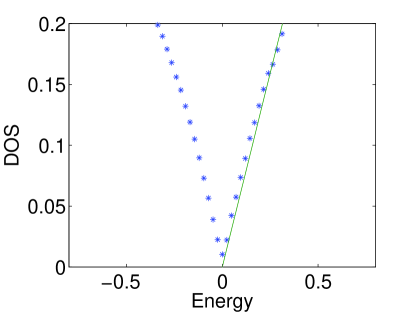
Figure 1: A comparison between the Coulomb gap obtained by the mean-field approximation, in two dimensions, and the theoretical prediction efros_SC of a linear gap with slope $\frac{2}{\pi e^{4}}$. The number of sites used was N=10000, and the Fermi energy was $E_{f}=0$ (half filling). The sites were uniformly distributed in a square, with ${e^{2}}n^{\frac{1}{2}}=1$, where $n$ is the density. The temperature was taken to be zero. The on-site disorder was distributed uniformly in the interval $[-\frac{1}{2},\frac{1}{2}]$. The y axis denotes the probability density of the energies $E_{i}$. The points are an average over 300 instances.

III Analysis using heuristic arguments

The heuristic arguments are based upon the low temperature approximation that the conductance follows efros :

$$\sigma\propto\gamma^{0}_{ij}\propto e^{-\left(r_{ij}/\xi-|E_{ij}|/T\right)}.$$ (2)

Where $\gamma^{0}_{ij}$ are two optimally coupled sites (i.e, with the highest rate between them). To maximize exponential functions it is sufficient to minimize the exponent even if the prefactors are not optimized. Indeed, it pays sometimes for the electron to hop a larger distance, thereby finding a state closer in energy and reducing the necessary inelastic energy transfer mott .

In the Hartree self consistent treatment it is legitimate to use the non-interacting concept of DOS and to ask how interactions modify it. To determine the shape of the interacting DOS, $\nu(E)$, (not to be confused with the non-interacting DOS $\nu_{0}$) we assume that the noninteracting and interacting energy-distance relation are equal, i.e., for two dimensions $E=e^{2}/r=1/\nu(E)r^{2}$. This yields the ES result $\nu(e)\sim E/e^{4}$. The tunneling DOS is suppressed at low energies due to interactions pollak_ ; efros2 ; sarvestani ; vojta ; pankov . Notice that $\nu(E)\sim\nu_{0}$ at $E_{C}=e^{4}\nu_{0}$, an energy above which the DOS becomes $\nu_{0}$. Hence $E_{C}$ determines the scale of the Coulomb gap.

Regarding the conductivity of the system, a-priori there could be four energy scales involved: the bandwidth $W$; the Coulomb energy $\frac{e^{2}}{r_{nn}}$, with $r_{nn}$ the average nearest-neighbor distance; the Coulomb energy over the localization length distance $E_{\xi}\equiv\frac{e^{2}}{\xi}$; and $\delta_{\xi}\equiv\frac{1}{\nu_{0}\xi^{2}}$, the level spacing in a box of size $\xi$. However, it is clear that the conductance as well as other physical quantities can not depend on $W$. Even in the limit of $W\longrightarrow\infty$, while keeping the (non-interacting) DOS at the Fermi level, $\nu_{0}$, constant, the expressions should be finite, since the energies involved in transport processes should occur near the Fermi energy $E_{F}$. Since $\frac{e^{2}}{r_{nn}}=\frac{E_{\xi}\sqrt{W}}{\sqrt{\delta_{\xi}}}$, this scale is also ruled out. Indeed, it is possible to express all the physical properties using $E_{\xi}$ and $\delta_{\xi}$. Using similar arguments we can understand the formula for $E_{C}$: Since the DOS is a static property of the system, determined by interaction energies on scales much larger than the localization length $\xi$, it cannot depend on $\xi$. The only energy scale that we can construct from $E_{\xi}$ and $\delta_{\xi}$ that does not depend on $\xi$ is $E_{\xi}^{2}/\delta_{\xi}=E_{C}$.

Optimizing Eq. (2) with the DOS described above yields Mott’s law for temperatures above a certain temperature and ES’s law efros for lower temperatures. The crossover temperature in two dimensions is given by :

$$T_{x}=E_{\xi}^{3}/\delta_{\xi}^{2}.$$ (3)

Note that this is consistent with the physical picture given previously, where it was shown that all physical properties must depend on $E_{\xi}$ and $\delta_{\xi}$.

So far we have reviewed simple heuristic arguments and discussed Mott’s and ES’s laws in a non-rigorous way. This enabled us to introduce the energy and length scale in the problem we study. In the rest of the paper we will perform analytical and numerical analysis of the Hartree approach, and show that it reproduces the non-rigorous results although it includes temperature and correlation effects that were omitted in the above heuristic approach.

IV Temperature dependence of the Coulomb gap

Determining the value of the finite DOS at the Fermi energy due to the effect of temperature is a problem which has not been settled yet: numerical investigations by [sarvestani, ] seem to be in disagreement with other theoretical predictions raikh . We hereby present the results of the mean-field theory. We calculate the density of states (DOS) at the Fermi-energy in the presence Coulomb interactions and finite temperature. For an infinite system at zero-temperature, the Efros-Shklovskii Coulomb gap will make the DOS vanish at the Fermi-energy. We know that finite-size effects will give rise to a finite DOS, proportional to $\frac{1}{\sqrt{N}}$coulomb_gap_mean_field . Let us assume we have a system large enough so that these finite-size effects will be negligible compared to the effects of the finite temperature. The finite-temperature mean-field equations are amir_glass :

$$E_{i}=\epsilon_{i}+\sum_{j\neq i}\left(\frac{1}{1+e^{\frac{E_{j}-E_{F}}{T}}}\ -Q_{b}\right)\frac{e^{2}}{r_{ij}}.$$ (4)

For half filling, $E_{F}=0$, and the positive background charge $Q_{b}=0.5$.

We have solved these equations numerically in two dimensions, and found a linear dependence of the DOS at $E_{f}$ as function of temperature. This is consistent with ref. [raikh, ]. The results are demonstrated in Fig. 2. Thus $\nu(E_{f})=\alpha T$, and since the Coulomb gap is washed out at a temperature of order $E_{C}$, we know that $\alpha\sim\frac{\nu_{0}}{E_{C}}$. For the data corresponding to Fig. 2 we find that $\alpha\approx 0.15$. In this case the ratio $\frac{\nu_{0}}{E_{C}}\approx 0.1$, which is consistent. We can now understand why this temperature dependence does not affect the crossover discussed in the previous section: while the finite-temperature contribution is linear in $T$, the optimal hop energy scales as $\sqrt{T}$ at low temperatures (before the crossover to Mott’s regime). One can check that even at the crossover temperature the finite-temperature correction to the DOS is not important.

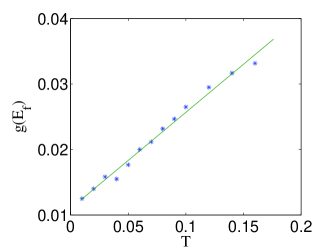
Figure 2: Density of states as a function of energy and temperature. Each graph is an average over 2000 iterations. For each, $N=1000$, and the ratio $\frac{T}{e^{2}n^{\frac{1}{2}}}$, where $T$ is the temperature, and $n$ the density, was varied between 0.01 and 0.58. The on-site disorder was taken uniform in the interval $[-5,5]$.

V Mean-field calculation of the conductance

We calculated the conductance numerically using the following scheme:

1. Find the equilibrium occupation number and energy associated with each electronic site within the mean-field picture, using Eq. (4). This takes the interactions into account, and the density-of-states obtained will manifest the Coulomb gap amir_glass .

2. Construct the Miller-Abrahams resistor network miller_abrahams ; ambegaokar . For a non-interacting problem, this is an exact method to find the resistance of the system by finding that of a certain resistor network. Here, the resistor between the sites $i$ and $j$ is given by $R_{ij}=\frac{kT}{e^{2}\gamma^{0}_{ij}}$, where $\gamma^{0}_{ij}$ are the equilibrium transition rates , which are calculated based on the energies $E_{i}$ and occupation numbers of the sites, see Eq. (1). Two sites which are close to each other in space and close in energy to the Fermi energy, will have a lower value of resistance between them: if the sites are far away in space, the overlap integrals will vanish exponentially. If the sites are far from the Fermi energy, they will be permanently full or empty, and will not contribute to the conductance.

3. Find the resistance of the system. This is done by solving for the energies (voltages) at the sites. In steady-state, the sum of currents into and out of each site must vanish. Expressing these currents in terms of the resistor network values and the energies yields a set of linear equations, solved numerically.

Executing the numerical procedure, we found that above a certain crossover temperature $T_{x}$, given by Eq. (3), approximately $e^{-{(\frac{T_{0}}{T})}^{\zeta}}$ behavior with $\zeta\sim 0.34\pm 0.01$ was observed for the resistivity, close to the Mott value in two dimensions of $\frac{1}{3}$. Below this temperature $\zeta\sim 0.49\pm 0.02$ was observed, in accordance with the Efros-Shklvoskii result finitesize . In the next section we give a scaling argument, which shows that:

$$\rm{log}\sigma\sim\delta_{\xi}/E_{\xi}\emph{f}(\emph{T}_{\emph{x}}/\emph{T}).$$ (5)

This allows us to collapse numerical data obtained for different sets of parameters. The crossover between the Mott and Efros-Shklovskii regimes is manifested in the asymptotics of $f(x)$. Fig. 3 demonstrates the crossover between the two regimes, and the data collapse, validating the scaling relation. We should emphasize, however, that the scaling relation is derived under certain assumptions: we assume that the temperature is low enough such that we do not have the trivial scenario of nearest-neighbor hopping. At $T>W$, we shall have nearest-neighbor hopping, and Mott’s law will not be valid: this gives a ’smoothing off’ of the Mott exponent, to a temperature independent regime. Thus, we do not expect complete data collapse for the regime where the temperature is larger than the disorder. Additionally, at very low temperatures, finite-size effects give rise to a finite DOS, and thus give rise to deviations from the Efros-Shklovskii hopping mechanism. Nevertheless, Fig. 3 shows clearly that data collapse is obtained. The least-squares fits in the asymptotic (linear) regimes gave the exponents discussed previously.

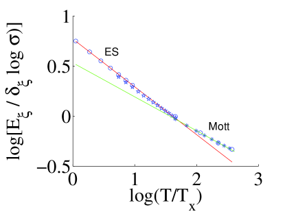
Figure 3: The crossover between ES and Mott VRH as the temperature is varied. Using the scaling relation of Eq. (5), we have collapsed data from different parameter sets onto the same master curve. We use N between 500 and 3000, and each point represents the average over 10 runs. We have verified that logarithmic averaging yields essentially the same results. The sites were chosen with uniform probability in a $\sqrt{N}X\sqrt{N}$ square with density $n=1$, and the energy scale was chosen such that $e^{2}n^{\frac{1}{2}}=1$. $n^{\frac{1}{2}}\xi$ was varied between 0.1 and 0.2, where $\xi$ is the localization length, and the on-site disorder was distributed uniformly in the interval $[-\frac{1}{2},\frac{1}{2}]$. The temperature axis was scaled according to the crossover temperature of Eq. (3). The conductance was scaled according to the scaling relation of Eq. (14) The lower temperature fit has an exponent of $0.49\pm 0.02$, consistent with the Efros-Shklovskii value of $1/2$ while the higher temperature fit has an exponent of $0.34\pm 0.01$, consistent with the Mott value of $1/3$. The lines are the best fits for the relevant data sets. In the Mott regime where the linear fit was taken the conductance changes by more than 3 orders of magnitude. In the ES regime, the conductance changes by more than 6 orders of magnitude.

VI Form of the crossover

The crossover between the Mott and ES regimes was discussed in references ora_VRH ; meir_scaling ; aharony_sarachik ; rosenbaum .

We shall now calculate the form of the crossover within our theoretical framework. We shall show that scaling is obeyed, for any dimensions, regardless of the details of the Coulomb gap. This generalizes previous work, for any DOS which depends only on the parameters $e^{2}$ and $\nu_{0}$. As previously explained, this is the generic form for the DOS. Notice that in principle the DOS is weakly dependent on temperature, and therefore this scaling relation is only an approximation. Let us proceed to the proof, for any dimension $d$. The basic equation connecting the energy $E$ and distance $r$ associated with a hop is obtained by requiring that the average number of sites within an area of order $r^{2}$ and energy lower than $E$ should be of order unity. Denoting the DOS as $\nu(E)$, this gives:

$$r^{2}\int_{0}^{E}\nu(E^{\prime})dE^{\prime}\sim 1.$$ (6)

The second equation comes from optimizing $\eta=\frac{r}{\xi}+\frac{E}{T}$. The optimal $\eta$ will determine the conductance of the system via $\log\sigma\sim-\eta$. Differentiating the first equation with respect to $r$ gives

$$\nu(E)=\frac{-d}{r^{d+1}}\frac{dr}{dE}.$$ (7)

Demanding the derivative of $\eta$ with respect to $r$ to vanish gives

$$\frac{1}{\xi}+\frac{1}{T}\frac{dE}{dr}=0.$$ (8)

Combining the last two equations yields

$$\nu(E)=\frac{\xi d}{\left[r\left(E\right)\right]^{d+1}T},$$ (9)

therefore:

$$\int^{E}\nu(E^{\prime})dE^{\prime}=\left(\frac{\nu(E)T}{d\xi}\right)^{\frac{d}{d+1}}.$$ (10)

To proceed, it is useful to define the function $\psi(E)=\frac{\int^{E}\nu(E^{\prime})dE^{\prime}}{({\frac{\nu(E)}{2})}^{\frac{d}{d+1}}}$. We have by assumption $\psi=\psi(E,\nu_{0},e^{2})$, and we obtain the equation:

$$\psi(E,\nu_{0},e^{2})={\left(\frac{T}{\xi}\right)}^{\frac{d}{d+1}}.$$ (11)

Since the dimensions of the LHS are $[energy/length]^{\frac{d}{d+1}}$, $\psi$ must have the form: $\psi=g(m)[E^{\frac{2}{d}}\nu_{0}^{\frac{2}{d}}e^{2}]^{\frac{d}{d+1}},$ where $m=\frac{E}{e^{\frac{2d}{d-1}}\nu_{0}^{\frac{1}{d-1}}}$ is a dimensionless combination of the parameters of $\psi$, and $g(m)$ is a certain function. Then the equation takes the form:

$$\left(\frac{E}{e^{\frac{2d}{d-1}}\nu_{0}^{\frac{1}{d-1}}}\right)=g^{-1}\left[{\left(\frac{T}{E^{\frac{2}{d}}\nu_{0}^{\frac{2}{d}}e^{2}\xi}\right)}^{\frac{d}{d+1}}\right].$$ (12)

We have an equation of the form $AE=f(BE),$ with $A=\frac{1}{e^{\frac{2d}{d-1}}\nu_{0}^{\frac{1}{d-1}}}$ and $B=e^{d}\nu_{0}(\frac{\xi}{T})^{\frac{d}{2}}$. Both $AE$ and $BE$ are dimensionless. The general solution will give us $E=\frac{1}{A}\phi(\frac{B}{A})$, for a certain function $\phi$. Plugging in the values of $A$ and $B$, we obtain

$$\frac{E}{T}=\frac{1}{(e^{2}\nu_{0})^{\frac{1}{d-1}}\xi}\theta(\frac{T_{x}}{T}),$$ (13)

with $T_{x}$ as defined by Eq. (3), and $\theta$ is a non-universal function, depending on the form of the DOS.

A similar dimensional analysis shows that $\frac{r}{\xi}$ follows an identical scaling law (but with a different function). Using the definition of $\eta$, we reach the conclusion that the conductance follows the proposed scaling, which can be written in terms of the energy scales $\delta_{\xi}$ and $E_{\xi}$ as:

$$\log\sigma\sim\left(\frac{\delta_{\xi}}{E_{\xi}}\right)f\left[\left(E_{\xi}^{d+1}/{\delta_{\xi}^{2}}\right)^{d-1}/{T}\right].$$ (14)

Notice that for $d=2$ we retrieve the crossover temperature of Eq. (3). The analysis did not assume anything on the shape of the DOS, other than the assumption that it is a function of $\nu_{0}$ and $e^{2}$: it does not have to contain a plateau or a power-law Coulomb gap. Nevertheless, if it does contain these features, $f$ must have asymptotics which correspond to the Mott and ES VRH: at $x\gg 1$ we have $f\propto x^{\frac{1}{d+1}}$, while for $x\ll 1$ we have $f\propto x^{\frac{1}{2}}$. An advantage of this calculation compared to other theories is that it allows one to complete the calculation for any DOS. Hence, it can be used by experimentalists to ’reverse-engineer’ and find the function $f$ that described the DOS from the conductivity measurements.

VII Summary

We have given a consistent Hartree-theory for the conductance of the electron glass. The long-range nature of the interactions should justify this approximation. In a previous work we showed the theory gives a linear Coulomb gap at zero temperature amir_glass , in accordance with other theories. Since the interactions are treated on a mean-field level, we can still use the single-particle DOS to characterize the conductance. This explains why the Coulomb gap indeed affects the conductance. Indeed, by numerically solving the Miller-Abrahams resistor network for the system, we found a crossover between the ES and Mott VRH regimes. Scaling is generically obeyed at the crossover, which we have derived analytically (neglecting interaction induced correlations), and compared to the numerics (which takes them into account). In future work we intend to incorporate many-electron tunneling into the theory, as well as study the out-of-equilibrium properties of the system.

We thank A. Aharony, A.L. Efros, O. Entin-Wohlman, Z. Ovadyahu and M. Pollak for useful discussions. This work was supported by a BMBF DIP grant as well as by ISF and BSF grants and the Center of Excellence Program. A.A. acknowledges funding by the Israel Ministry of Science and Technology via the Eshkol scholarship program.

References

- (1) B. Shklovskii and A. Efros, Electronic properties of doped semiconductors (Springer-Verlag, Berlin, 1984).
- (2) Electron-electron interactions in disordered systems, edited by A. L. Efros and M. Pollak (North-Holland, Amsterdam, 1985).
- (3) V. F. Gantmakher, Electrons and Disorder in Solids (Oxford University Press, Oxford, 2005).
- (4) Hopping Transport in Solids, edited by M. Pollak and B. I. Shklovskii (Elsevier, London, 1990).
- (5) N. F. Mott, Phil. Mag. 19, 835 (1969).
- (6) M. Pollak, Discuss. Faraday Soc. 50, 13 (1970).
- (7) A. L. Efros and B. I. Shklovskii, J. Phys. C 8, L49 (1975).
- (8) J. G. Massey and M. Lee, Phys. Rev. Lett. 75, 4266 (1995).
- (9) V. Y. Butko, J. F. DiTusa, and P. W. Adams, Physical Review Letters 84, 1543 (2000).
- (10) A. Mobius et al., J. Phys. C 16, 6491 (1983), A. Mobius et al., J. Phys. C 18, 3337 (1985), A. Mobius, J. Phys. C 18, 4639 (1985), W. N. Shafarman, D. W. Koon, and T. G. Castner, Phys. Rev. B 40, 1216 (1989), Y. Zhang, P. Dai, M. Levy, and M. P. Sarachik, Phys. Rev. Lett. 64, 2687 (1990), R. Rosenbaum, Phys. Rev. B. 44, 3599 (1991), Y. Liu, B. Nease, K. A. McGreer, and A. M. Goldman, Europhys. Lett. 19, 409 (1992) I. Shlimak, M. Kaveh, M. Yosefin, M. Lea and P. Fozooni, Phys. Rev. Lett. 68, 3076 (1992), U. Kabasawa et al., Phys. Rev. Lett. 70, 1700 (1993), J. Lam, M. D’Iorio, D. Brown, and H. Lafontaine, Phys. Rev. B 56, R12741 (1997), M. P. Sarachik and P. Dai, Europhys. Lett. 59, 100 (2002).
- (11) M. Pollak, Phys. Stat. Sol. (c) 5, 667 (2008).
- (12) M. Grunewald, B. Pohlmann, L. Schweitzer, and D. Wurtz, J. Phys. C: Solid State Phys., 15, L1153 (1982).
- (13) A. Amir, Y. Oreg, and Y. Imry, Phys. Rev. B 77, 165207 (2008).
- (14) M. R. A. Shegelski and D. S. Zimmerman, Phys. Rev. B 39, 13411 (1989).
- (15) F. Goedsche, phys. stat. sol. (b) 140, 225 (1987).
- (16) A. Amir, Y. Oreg, and Y. Imry, to appear in PRL.
- (17) O. Entin-Wohlman, Y. Gefen, and Y. Shapira, J. Phys. C 16, 1161 (1983).
- (18) Y. Meir, Phys. Rev. Lett. 77, 5265 (1996).
- (19) A. Aharony, Y. Zhang, and M. P. Sarachik, Phys. Rev. Lett. 68, 3900 (1992).
- (20) R. Rosenbaum, N. V. Lien, M. R. Graham, and M. Witcomb, J. Phys.: Condens. Matter 9, 6247 (1997).
- (21) M. Goethe and M. Palassini, Phys. Rev. Lett. 103, 045702 (2009).
- (22) A. L. Efros, J. Phys. C: Solid State Phys 9, 2021 (1976).
- (23) M. Sarvestani, M. Schreiber, and T. Vojta, Phys. Rev. B 52, R3820 (1995).
- (24) F. Epperlein, M. Schreiber, and T. Vojta, Phys. Rev. B 56, 5890 (1997).
- (25) M. Muller and S. Pankov, Phys. Rev. B. 75, 144201 (2007).
- (26) A. A. Mogilyanski and M. E. Raikh, Sov. Phys. JETP 68, 1081 (1989).
- (27) A. Miller and E. Abrahams, Phys. Rev. 120, 745 (1960).
- (28) V. Ambegaokar, B. I. Halperin, and J. S. Langer, Phys. Rev. B 4, 2612 (1971).
- (29) At low temperatures finite size effects will give rise to a finite DOS at the Fermi energy, modifying this picture and raising the conductance. These were also seen numerically.