The magnetic field particle-hole excitation spectrum
in doped graphene and in a standard two-dimensional electron gas

Abstract

The particle-hole excitation spectrum for doped graphene is calculated from the dynamical polarizability. We study the zero and finite magnetic field cases and compare them to the standard two-dimensional electron gas. The effects of electron-electron interaction are included within the random phase approximation. From the obtained polarizability, we study the screening effects and the collective excitations (plasmon, magneto-excitons, upper-hybrid mode and linear magneto-plasmons). We stress the differences with the usual 2DEG.

I Introduction

The particle-hole excitation spectrum (PHES) of a material is an extremely useful ingredient for the understanding of its electronic properties, namely at low energies. It reveals, for example, collective modes such as the plasmon, the electric polarizability of the material, and the screening properties of the electrons in it. In this paper, we review the particular PHES of two-dimensional electron systems, both for non-relativistic electrons in a usual two-dimensional electron gas (2DEG)Ando et al. (1982) and for massless electrons in graphene.Neto et al. (2009) The main focus of the present review article is on the PHES and the collective modes of doped graphene in a strong perpendicular magnetic field in the integer quantum Hall regime.Iyengar et al. (2007); Shizuya (2007); Bychkov and Martinez (2008); Tahir and Sabeeh (2008); Berman et al. (2008); Roldán et al. (2009); Fischer et al. (2009) For pedagogical reasons, we compare them to the corresponding results of the 2DEGGiuliani and Vignale (2005); Kallin and Halperin (1984) as well as to the PHES in graphene without a magnetic field, which has been theoretically studied in detail recently.Shung (1986); Ando (2006a); Wunsch et al. (2006); Hwang and Sarma (2007)

The main difference between the PHES in graphene and that in the 2DEG, in a strong magnetic field $B$, stems from the quantization of the electrons’ kinetic energy in Landau levels (LL): these levels are equidistantly spaced in the case of non-relativistic electrons in the 2DEG, $\epsilon_{n}^{\rm 2DEG}=\omega_{c}(n+1/2)$, in terms of the cyclotron frequency $\omega_{c}=eB/m_{b}$, where $m_{b}$ is the band mass (we use a system of units such that $\hbar\equiv 1$). In contrast to this, the LLs in graphene occur in two copies as a consequence of the two energy bands ($\lambda=+$ for the conduction and $\lambda=-$ for the valence band), and their level spacing decreases with increasing LL quantum number $n$,

$$\epsilon_{\lambda,n}=\lambda\epsilon_{n}=\lambda\frac{v_{\rm F}}{l_{B}}\sqrt{2n}\propto\lambda\sqrt{Bn}\,.$$ (1)

where $v_{\rm F}$ is the Fermi velocity in graphene and $l_{B}=1/\sqrt{eB}$ is the magnetic length. This difference in LL quantization as well as the absence of backscattering due to the chirality properties of electrons in graphene Shon and Ando (1998) yield a strikingly different PHES for graphene when compared to the 2DEG. Whereas, in the latter, the collective excitations are dominated by essentially horizontal weakly-dispersing magneto-excitons,Kallin and Halperin (1984) in addition to the upper hybrid mode, those in graphene are linear magneto-plasmons Roldán et al. (2009) that disperse roughly parallel to an energy line $\omega=v_{\rm F}q$, as a function of the wave vector $q$. The precursors of these modes are already visible in the PHES for non-interacting electrons and acquire coherence once electron-electron interactions are taken into account, e.g. on the level of the random-phase approximation (RPA).

The paper is organized as follows. In Sec. II, we introduce the basic expressions for the polarization function of graphene in a strong magnetic field. The intermediate steps of the derivation may be found in Appendix A. Section III is devoted to a discussion of the PHES in the standard 2DEG for non-relativistic electrons, whereas that for doped graphene is presented in Sec. IV. Both sections comprise also a short review of the $B=0$ case. In Sec. V, we aim at a physical interpretation of main features of the two different PHES in a strong magnetic field within a wave-function analysis, and the screening properties in the static limit are reviewed in Sec. VI.

II Polarizability

The Hamiltonian for graphene in a magnetic field can be expressed as ${\cal H}_{0}^{K}=v_{\rm F}\,{\boldsymbol{\pi}}\cdot{\boldsymbol{\sigma}}$ for the $K$ valley and ${\cal H}_{0}^{K^{\prime}}=v_{\rm F}\,{\boldsymbol{\pi}}\cdot{\boldsymbol{\sigma}^{*}}$ for the $K^{\prime}$ valley, where ${\boldsymbol{\sigma}=(\sigma^{x},\sigma^{y})}$ are Pauli matrices, and ${\boldsymbol{\pi}}={\bf p}+e{\bf A}$ is the gauge-invariant momentum with ${\bf p}=-i{\boldsymbol{\nabla}}$, and $\bf A$ is the vector potential. In the symmetric gauge, the latter reads ${\bf A}=(-By/2,Bx/2,0)$, where $B$ is the modulus of the magnetic field that we choose in the $z$-direction. The Fermi velocity $v_{\rm F}=3ta/2$ is expressed in terms of the nearest-neighbor hopping integral $t\simeq 3$ eV and the carbon-carbon distance $a\simeq 1.4$ Å. The eigenstates components $|\psi_{\zeta\alpha;\lambda,n,\ell}\rangle$ are:

$$|\psi_{+A;\lambda,n,\ell}\rangle=|\psi_{-B;\lambda,n,\ell}\rangle =-i\lambda 1^{*}_{n}|n-1,\ell\rangle$$

$$|\psi_{-A;\lambda,n,\ell}\rangle=|\psi_{+B;\lambda,n,\ell}\rangle =2^{*}_{n}|n,\ell\rangle$$ (2)

where $n$ is a positive integer, $\lambda=\pm$ for states of positive/negative energy and $\lambda=0$ for $n=0$. The corresponding eigenenergies are given in Eq. (1). The index $\zeta=+(-)$ denotes electrons in the ${\rm K}({{\rm K}^{\prime}})$ valleys and $\alpha=A(B)$ the $A(B)$ sublattice component of the electronic wave function. We have furthermore introduced the simplified notation $1^{*}_{n}=\sqrt{(1-\delta_{n,0})/2}$ and $2^{*}_{n}=\sqrt{(1+\delta_{n,0})/2}$. Here the quantum number $n$ labels the LL, whereas the other quantum number $\ell$, which determines the LL degeneracy, varies from $0$ to $N_{B}-1$, with $N_{B}={\cal A}n_{B}={\cal A}/2\pi l_{B}^{2}$, in terms of the total sample surface $\cal A$ . The states $|n,\ell\rangle$ are the eigenvectors of the Hamiltonian

$$\mathcal{H}_{0}^{\rm 2DEG}=\frac{\pi_{x}^{2}+\pi_{y}^{2}}{2m_{b}}$$ (3)

for the standard 2DEG in a magnetic field.

The bare polarization function

$$i\Pi^{0}({\bf q},\omega)=\int\frac{d\omega^{\prime}d{\bf k}}{(2\pi)^{3}}\,{\rm Tr}\left[G^{0}({\bf k},\omega^{\prime})G^{0}({\bf k}+{\bf q},\omega^{\prime}+\omega)\right].$$ (4)

may be calculated with the help of the Green’s functions $G^{0}({\bf k},\omega)$ for non-interacting electrons [see Eq. (25)] and reads, for the case of a strong magnetic field,Roldán et al. (2009)

$$\Pi^{0}({\bf q},\omega)=\sum_{\lambda\lambda^{\prime}}\sum_{n,n^{\prime}}\frac{\Theta(\lambda^{\prime}\xi_{n^{\prime}})-\Theta(\lambda\xi_{n})}{\lambda\xi_{n}-\lambda^{\prime}\xi_{n^{\prime}}+\omega+i\delta}{\cal\overline{F}}_{nn^{\prime}}^{\lambda\lambda^{\prime}}({\bf q}).$$ (5)

The expression of the functions ${\cal\overline{F}}_{nn^{\prime}}^{\lambda\lambda^{\prime}}({\bf q})$ and the details of the calculation may be found in Appendix A. $\Pi^{0}$ contains two separate contributions,

$$\Pi^{0}({\bf q},\omega)=\sum_{n=1}^{N_{F}}\Pi_{n}^{\lambda_{F}}({\bf q},\omega)+\Pi^{vac}({\bf q},\omega).$$ (6)

The vacuum contribution $\Pi^{vac}({\bf q},\omega)$ takes into account inter-band processes, whereas $\sum_{n=1}^{N_{F}}\Pi_{n}^{\lambda_{F}}({\bf q},\omega)$ represents intra-band contributions when the Fermi energy $\epsilon_{F}=\epsilon_{N_{F}}$ lies in the conduction band, as we assume implicitly from now on.

II.1 Effect of electron-electron interaction

From $\Pi^{0}({\bf q},\omega)$ we can calculate the renormalized polarization function in the RPA, which is defined as

$$\Pi^{RPA}({\bf q},\omega)=\frac{\Pi^{0}({\bf q},\omega)}{\varepsilon^{RPA}({\bf q},\omega)}=\frac{\Pi^{0}({\bf q},\omega)}{1-v({\bf q})\Pi^{0}({\bf q},\omega)}$$ (7)

where $v({\bf q})$ is the unscreened two-dimensional Coulomb potential in momentum space

$$v({\bf q})=\frac{2\pi e^{2}}{\varepsilon_{b}|{\bf q}|}$$ (8)

in terms of the background dielectric constant $\varepsilon_{b}$, and $\varepsilon^{RPA}({\bf q},\omega)=1-v({\bf q})\Pi^{0}({\bf q},\omega)$ is the dielectric function. Long-range electron-electron interaction usually leads to the appearance of collective modes in the spectrum, such as the plasmon, the dispersion of which is defined from the zeros of the dielectric function

$$\varepsilon^{RPA}({\bf q},\omega)=0.$$ (9)

Collective modes will be discussed in detail for both, graphene and a standard 2DEG, in the following sections.

III Particle-hole excitation spectrum of a standard 2DEG

In this section we briefly review the results for the PHES in a 2DEG and start with the case of zero magnetic field. The polarization function Eq. (4) for a system of free electrons with parabolic band $\varepsilon_{{\bf k}}=k^{2}/2m_{b}$ can be expressed, after some manipulation, as Giuliani and Vignale (2005)

$$\Pi^{0}_{\rm 2DEG}({\bf q},\omega)=\rho(\epsilon_{F})\frac{k_{F}}{q}\!\!\!\! \!\!\!\!\left[\Psi\left(\frac{\omega+i\delta}{v_{\rm F}q}-\frac{q}{2k_{F}}\right)\right.$$ (10)

$$\left.-\Psi\left(\frac{\omega+i\delta}{v_{\rm F}q}+\frac{q}{2k_{F}}\right)\right]$$

where $\rho(\epsilon_{F})$ is the density of states at the Fermi level, $\delta\sim\tau^{-1}$ accounts for a finite life time of the quasiparticles, and $\Psi(z)=z-{\rm sgn}({\rm Re}\,z)\sqrt{z^{2}-1}$. In Fig. 1(a) we show a density plot of ${\rm Im}\,\Pi^{0}_{\rm 2DEG}$. From the imaginary part of $\Pi^{0}$ we can obtain the PHES, which is the region of the momentum-energy plane where it is possible to excite electron-hole pairs. This region is defined, for a non-interacting electron gas in the absence of a magnetic field, as the continuum of Fig. 1 with non-zero ${\rm Im}\,\Pi^{0}$, which corresponds (for $\delta\rightarrow 0$) to the region delimited by the solid black lines. The boundaries of the spectrum are defined by $\max[0,\omega_{-}(q)]\leq|\omega|\leq\omega_{+}(q)$, where $\omega_{\pm}(q)=q^{2}/2m_{b}\pm v_{\rm F}q$, in terms of the Fermi velocity $v_{\rm F}=\partial\epsilon/\partial k|_{k_{F}}=k_{F}/m_{b}=\sqrt{2\epsilon_{F}/m_{b}}$, which in contrast to graphene depends on $\epsilon_{F}$. Notice that this PHES is not uniform, but presents some structure. Apart from the quasi-homogeneous yellow region, two other zones are worth describing: the blue one, with a strong spectral weight, which is the precursor of the plasmon mode, as we will see below, and the almost red low energy region, with a very weak spectral weight and which, in a 1D system, would belong to the forbidden zone of the spectrum for particle-hole excitations.

Electron-electron interactions lead to the appearance of a collective mode, the plasmon, which can be captured within the RPA. The imaginary part of $\Pi^{RPA}({\bf q},\omega)$, shown in Fig. 1, reveals above the continuum boundaries a well-defined peak centered at $\omega=\omega_{p}$, the frequency of the plasmon mode. The broadening of the peak depends on the value of $\delta\sim\tau^{-1}$ and is due, e. g., to scattering of electrons by disorder. The dispersion relation of the plasmon may be calculated from the zeros of the RPA polarization function. From the $q\rightarrow 0$ and $\omega\ll v_{\rm F}q$ expansion of the polarization function, the long wavelength limit of the plasmon dispersion is found to beStern (1967)

$$\omega_{p}(q)\simeq\sqrt{\frac{2e^{2}\epsilon_{\rm F}}{\varepsilon_{b}}q+\frac{3}{4}v_{\rm F}^{2}q^{2}},$$ (11)

where the Fermi energy in a 2DEG with a parabolic band can be expressed in terms of the the uniform density of electrons $n_{el}$ as $\epsilon_{\rm F}=\pi n_{el}/m_{b}$. Furthermore, from the analytic solution of Eq. (9), an exact dispersion relation of the plasmon mode may be obtained to all orders in $q$ (see Ref. Czachor et al., 1982). At low energies, it disperses as $\sqrt{q}$, and at some critical wave vector $q_{c}$, the mode touches the electron-hole continuum. This critical value may be obtained from Czachor et al. (1982)

$$\frac{(q_{c}/k_{F})^{2}}{\sqrt{2}r_{s}}+\frac{(q_{c}/k_{F})^{3}}{4r_{s}^{2}}=1,$$ (12)

in terms of the dimensionless interaction parameter $r_{s}\equiv 2m_{b}e^{2}/\varepsilon_{b}k_{F}$. Above $q_{c}$, the plasmon disperses roughly parallel to the boundary of the particle-hole continuum while being Landau-damped due to its decay into electron-hole pairs [see Fig. 1].

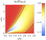
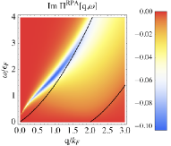
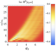
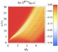
Figure 1: Density plot of ${\rm Im}\Pi({\bf q},\omega)$. Plots (a) corresponds to non-interacting polarization of a 2DEG, Eq. (10), whereas (b) accounts also for electron-electron interactions in the RPA. Plots (c) and (d) show the imaginary part of the non-interacting and RPA polarization function, respectively, of a 2DEG in a magnetic field. In (a) and (b) we have used $\delta=0.2\varepsilon_{F}$. In (c) and (d), $N_{F}=3$ and $\delta=0.2\omega_{c}$. In (b) and (d), we have used $r_{s}\simeq 3$.

In the presence of a strong magnetic field perpendicular to the 2DEG, the bare polarizability can be expressed asKallin and Halperin (1984)

$$\Pi^{0}_{2DEG}({\bf q},\omega)=\sum_{m=1}^{N_{c}}{\sum}^{\prime}\frac{{\cal F}_{n,m}({\bf q})}{\omega-m\omega_{c}+i\delta}+(\omega^{+}\rightarrow-\omega^{-})$$ (13)

where $\sum^{\prime}=\sum_{n=\max(0,N_{F}-m)}^{N_{F}-1}$ and $\omega^{+}\rightarrow-\omega^{-}$ indicates the replacement $\omega+i\delta\rightarrow-\omega-i\delta$. The form factor due to the wave-function overlap is

$${\cal F}_{n,m}({\bf q})=\frac{e^{-\frac{q^{2}l_{B}^{2}}{2}}}{2\pi l_{B}^{2}}\frac{n!}{(n+m)!}\left(\frac{q^{2}l_{B}^{2}}{2}\right)^{m}\left[L_{n}^{m}\left(\frac{q^{2}l_{B}^{2}}{2}\right)\right]^{2}.$$ (14)

A density plot of ${\rm Im}\,\Pi^{0}$ is shown in Fig. 1 for $N_{F}=3$. In the presence of a strong magnetic field, ${\rm Im}\,\Pi^{0}({\bf q},\omega)$ is a sum of Lorentzian peaks centered at $\omega=m\omega_{c}$, with $m\equiv n^{\prime}-n\geq 1$, the difference between the LL indices of the electron $n^{\prime}$ and the hole $n$. Therefore the PHES is chopped into horizontal lines, separated by a constant energy $\omega_{c}$. The width of each horizontal line is proportional to the disorder broadening of the Landau levels. (The peaks become $\delta$-functions in the clean limit $\delta\rightarrow 0^{+}$.) Notice that within each horizontal line, the spectral weight is not homogeneously distributed; one observes indeed a superstructure of $N_{F}+1$ brighter regions in Fig. 1 following lines parallel to the edges of what used to be the particle-hole continuum in the zero-field case. These edges delimit, also for non-zero values of the magnetic field, the PHES region of non-vanishing spectral weight.

In the presence of electron-electron interactions, the density fluctuation spectrum of a 2DEG at integer filling factors is dominated by a single set of collective modes, known as horizontal magneto-excitons. The frequency of these modes tend to $m\omega_{c}$ (where $m$ is a positive integer) in the long wavelength limit, and their dispersion was calculated by Kallin and Halperin in the RPA and in the time-dependent Hartree-Fock approximation.Kallin and Halperin (1984) In Fig. 1 we show the RPA excitation spectrum for $r_{s}\equiv 2m_{b}e^{2}/\varepsilon_{b}k_{F}\approx 3$. Furthermore, one notices that the plasmon energy is renormalized by the magnetic field and evolves into the so called upper hybrid mode. Its dispersion relation can be expressed asChiu and Quinn (1974)

$$\omega_{uh}^{2}(q)=\omega_{p}^{2}(q)+\omega_{c}^{2},$$ (15)

where an approximate expression for $\omega_{p}(q)$ has been given in Eq. (11).

IV Particle-hole excitation spectrum of doped graphene

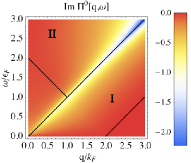
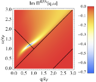
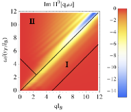
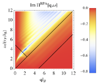
Figure 2: Same as Fig. 1 but for the case of graphene. The solid lines delimitate the boundaries of the PHES. Region I corresponds to the intra-band and region II to the inter-band region of the PHES of doped graphene. In (a) and (b), $\delta=0.1\varepsilon_{F}$. In (c) and (d), $\delta=0.2v_{\rm F}/l_{B}$. In (b) and (d), we have used $r_{s}=1$.

We start with a review of the polarization function in the absence of a quantizing magnetic field, which turns out to be useful in the understanding of the PHES also at $B\neq 0$. In the continuum approximation, the non-interacting polarization function at zero temperature can be calculated from

$$\Pi^{0}({\bf q},\omega)=\frac{g}{{\cal A}}\sum_{{\bf k},\lambda,\lambda^{\prime}}\frac{\Theta(\lambda^{\prime}\xi_{{\bf k}+{\bf q}})-\Theta(\lambda\xi_{{\bf k}})}{\lambda\xi_{{\bf k}}-\lambda^{\prime}\xi_{{\bf k}+{\bf q}}+\omega+i\delta}F_{\lambda\lambda^{\prime}}({\bf k},{\bf k}+{\bf q}),$$ (16)

where $\lambda\xi_{{\bf k}}=\lambda v_{\rm F}|{\bf k}|-\epsilon_{\rm F}$ is the quasiparticle energy relative to the Fermi level, $g=g_{s}g_{v}=4$ accounts for spin and valley degeneracy and

$$F_{\lambda\lambda^{\prime}}({\bf k},{\bf k}+{\bf q})=\frac{1+\lambda\lambda^{\prime}\cos\theta_{{\bf k},{\bf k}+{\bf q}}}{2}$$ (17)

is the chirality factor or wave function overlap, where $\theta_{{\bf k},{\bf k}+{\bf q}}$ is the angle between ${\bf k}$ and ${\bf k}+{\bf q}$. $\Pi^{0}({\bf q},\omega)$ was calculated for undoped graphene in Ref. González et al., 1994, where it was found that ${\rm Im}\,\Pi^{0}({\bf q},\omega)\sim q^{2}(\omega^{2}-v_{\rm F}^{2}q^{2})^{-1/2}$, which implies that the massless non-interacting electrons in graphene have an infinite response at the threshold $\omega=v_{\rm F}q$. The reason for this behavior is twofold: first the threshold is determined by the linear dispersion relation and second, the chirality factor (17) suppresses backscattering in graphene. This feature is still present in doped graphene, although the form of the polarization function is richer than in the absence of doping,Shung (1986); Wunsch et al. (2006); Hwang and Sarma (2007) as may be seen in Fig. 2, where we show a density plot of $\Pi({\bf q},\omega)$ for doped graphene at $B=0$. One notices that most of the spectral weight is actually concentrated around $\omega=v_{\rm F}q$, as one would expect from the suppression of backscattering ($2k_{F}$ processes). This is similar to the case of zero doping.

In doped graphene, however, there are two regions of non-vanishing spectral weight which arise from intra-band (region I) and inter-band processes (region II). These two regions are separated by the diagonal line $\omega=v_{\rm F}q$. For zero doping, there are naturally only inter-band processes. The intra-band contributions are restricted to region I the boundaries of which are $\max(0,v_{\rm F}q-2\varepsilon_{F})\leq|\omega|\leq v_{\rm F}q$. This is the only kind of processes present in the 2DEG, discussed in the preceding section. The features of this zone are, apart from the different shape of the boundaries in the two cases, similar to the PHES of the 2DEG, although the spectral weight is no longer homogeneously distributed within this region but vanishes when approaching the right boundary as a consequence of the chirality factor. Inter-band particle-hole excitations are restricted to region II in the PHES, with boundaries $|\omega|\geq\max(v_{\rm F}q,-v_{\rm F}q+2\varepsilon_{F})$. Indeed, the inter-band excitation of lowest energy needs to overcome the Fermi energy, which is therefore the lower bound of region II and which approaches zero in undoped graphene, where the region of inter-band excitations covers the whole part $\omega>v_{\rm F}q$ of the spectrum. Furthermore, due to the presence of two energy bands, there is the possibility of direct transitions from the valence to the conduction band with $q=0$ momentum transfer. The $q=0$ transition of lowest energy involves an energy cost that is twice the Fermi energy, which yields a gapped region in the PHES in Fig. 2(a), defined by $0<\omega<2\varepsilon_{F}$. Notice however that the $q=0$ transition is suppressed due to the chirality factor (17).

The real and imaginary parts of the polarization function are related via the Kramers-Kronig relations. Their behavior is shown in Fig. 3 where we plot $-\Pi^{0}(q_{0},\omega)$ for different wave-vectors $q_{0}$ for both, 2DEG [plots (a) and (b)] and graphene [plots (c) and (d)]. We note that most of the spectral weight (region with non-zero ${\rm Im}\,\Pi^{0}$) of graphene is concentrated near $\omega=v_{\rm F}q$ (due to the absence of backscattering), whereas in the 2DEG it is more uniformly distributed.

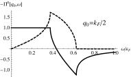
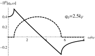
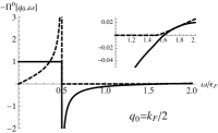
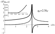
Figure 3: Polarization function of a 2DEG [plots (a) and (b)] and graphene [(c) and (d)] for different wave-vectors $q_{0}$. Solid lines set for ${\rm Re}\,\Pi^{0}(q_{0},\omega)$ and dashed lines for ${\rm Im}\,\Pi^{0}(q_{0},\omega)$. $q_{0}=0.5k_{F}$ in (a) and (c), and $q_{0}=2.5k_{F}$ in (b) and (d). All the plots are done for $\delta\rightarrow 0^{+}$.

When electron-electron interactions are included in the problem, RPA has been shown to capture the essential physics for doped graphene:Wunsch et al. (2006); Hwang and Sarma (2007); Sabio et al. (2008) contrary to undoped graphene, the density of states is finite at the Fermi level once doping moves $\epsilon_{\rm F}$ away from the Dirac points. However, due to the vanishing density of states at the Dirac point,Katsnelson (2006) the RPA description is incomplete for undoped graphene,Gangadharaiah et al. (2008) and it is therefore necessary to consider another class of diagrams in perturbation theory (such as ladder-type vertex corrections) which lead to a plasmon resonance below the threshold $\omega<v_{\rm F}q$. For doped graphene, the poles of $\Pi^{RPA}({\bf q},\omega)$ define the dispersion of a collective plasmon mode, which has the same long-wavelength $\sqrt{q}$ behavior as the plasmon in the 2D electron gas studied in the preceding section [see Eq. (11) and Fig. 2]. An approximate dispersion relation of the plasmon in a single layer of doped graphene was calculated in Ref. Shung, 1986 in the framework of a study of intercalated graphite and was found to coincide with Eq. 11, in which the Fermi energy is now related to the uniform density of electrons $n_{el}$ as $\epsilon_{\rm F}=v_{\rm F}k_{F}=v_{\rm F}\sqrt{\pi n_{el}}$. Within the previous approximation, the plasmon mode enters the inter-band region of the PHES at a momentum

$$q_{c}=4k_{F}\left(2+r_{s}-\sqrt{r_{s}^{2}+4r_{s}+3}\right),$$ (18)

where $r_{s}\equiv e^{2}/\varepsilon_{b}v_{\rm F}$. Note that $r_{s}$ is density-dependent in the 2DEG whereas it is scale-invariant in graphene. One important difference with respect to the 2DEG case is that only for $\omega>v_{\rm F}q$ it is possible to have a solution for the plasmon dispersion $1=v(q){\rm Re}\,\Pi^{0}(q,\omega)$, because ${\rm Re}\,\Pi^{0}({\bf q},\omega)<0$ for $\omega<v_{\rm F}q$ [Fig. 3(c)-(d)]. As a consequence, the collective plasmon mode in graphene at zero magnetic field can only be damped when decaying into inter-band (and never into intra-band) particle-hole excitations. Notice also the difference with respect to the 2DEG case, where the plasmon mode is damped once its dispersion touches, at some critical wave-vector, the boundary of the PHES. The RPA dispersion relation of the 2DEG plasmon itself, however, never enters the intra-band continuum. In the case of graphene, even if the plasmon enters the inter-band region of the PHES at a well defined wave-vector approximately given by Eq. (18), the mode continues to exist in a rather large region of the inter-band continuum.Polini et al. (2008) Recently it has been arguedPolini et al. (2009) that, due to the lack of Galilean invariance in graphene, exchange interactions, which are not included in the RPA, renormalize the plasmon dispersion of doped graphene in the long-wavelength limit. This renormalization is due primarily to non-local inter-band exchange interactions, which reduce the plasmon frequency relative to the RPA value.

We study now the PHES of doped graphene in the presence of a strong magnetic field perpendicular to the sample. As in the zero magnetic field case, the strong contribution to the polarization comes from the divergence of $\Pi^{0}({\bf q},\omega)$ at $\omega=v_{\rm F}q$, as it can be seen in Fig. 2. The effect of the LL wave-function overlap ${\cal\overline{F}}_{nn^{\prime}}^{\lambda\lambda^{\prime}}({\bf q})$ [Eq. (27)] is appreciable, in the intra-band region of the spectrum in Fig. 4(b), where we see that the intensity of the modes is larger near the threshold $v_{\rm F}q$ and practically unappreciable near the second boundary of the intra-band PHES $\omega=\max(0,v_{\rm F}q-2\epsilon_{\rm F})$. But in addition, ${\rm Im}\,\Pi^{0}({\bf q},\omega)$ is finite not only in the intra-band region, but also in the zones of Fig. 2 with a finite weight, as the yellow stripes above and below $\omega=v_{\rm F}q$. This form of the PHES is due to both, the LL structure of the spectrum (1) and the presence of inter-band excitations that lead to the mentioned stripes in region II of the PHES. The most salient feature that we find comparing the PHES of a 2DEG [Fig. 1] to that of graphene [Fig. 2] in a magnetic field, is that in the former the spectrum is composed of horizontal and equidistant non-dispersive lines, while in the latter these modes are not visible, and the important modes are the diagonal lines parallel to the threshold $\omega=v_{\rm F}q$.

This particular feature of the PHES of graphene in a strong magnetic field may be understood in the following manner. Notice first that, in contrast to the 2DEG with its equally spaced LLs, the spacing of the relativistic LLs in graphene (1) decreases at higher energies. In a fixed energy window at high energies, there are therefore more possible inter-LL excitations from the level $n$ in the band $\lambda$ to $n^{\prime}$ in the conduction band, of energy $\omega_{n,n^{\prime}-n}^{\lambda}=\sqrt{2}(v_{\rm F}/l_{B})(\sqrt{n^{\prime}}-\lambda\sqrt{n})$, than at lower energies. Notice further that above an energy of $\epsilon_{F}$ also inter-band transitions with $\lambda=-$ contribute. Even for small values of $\delta$, i.e. in clean samples, neighboring LL transitions overlap in energy such that the horizontal lines, which dominate the PHES of the 2DEG in a strong magnetic field [Fig. 1], are blurred. At fixed energy, the spectral weight is again not homogeneously distributed. This is a consequence of the wave-function overlap between the electron and the hole, as we discuss in more detail in the following section.

The above-mentioned dispersive modes in graphene, acquire coherence once electron-electron interactions are taken into account. This can be seen in Fig. 2, which shows the RPA polarization function, and where the dispersive diagonal lines are now clearly distinguishable. We will refer to them as linear magneto-plasmons. In the inter-band region of the PHES, the number of linear magneto-plasmons depends on the high energy cutoff $N_{c}$. We should keep in mind that the RPA is a good approximation for describing the long-wavelength part of the spectrum, but fails in reproducing many of the physical properties of a system in the short-wavelength regime. The dispersion of the collective modes at short-wavelength is renormalized when diagrammatic contributions beyond the RPA are taken into account. In particular, the inclusion of ladder diagrams, which account for the direct interaction between the electron and hole, as well as the exchange terms, lead to the excitonic and exchange shifts in the magneto-exciton dispersion.Kallin and Halperin (1984); Iyengar et al. (2007); Bychkov and Martinez (2008)

V Structure of the particle-hole excitation spectrum: a wave-function analysis

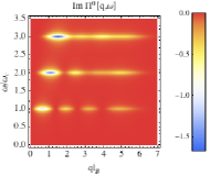
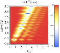
Figure 4: Density plot of ${\rm Im}\,\Pi^{0}({\bf q},\omega)$ in the low energy sector. Plot (a) corresponds to a 2DEG and plot (b) to graphene. We have used $N_{F}=3$ and $\delta=0.05$ in units of $\omega_{c}$ and $v_{\rm F}/l_{B}$, respectively. Islands (see text) are clearly visible in the $\omega=\omega_{c}$ horizontal line in (a) and in every horizontal line in (b).

The boundaries of the PHES in a magnetic field may be understood by considering an electron-hole pair and treating the cyclotron motion of both the electron and the hole in a semiclassical limit. The boundaries are related to the region in real space where the electron and hole cyclotron orbits may overlap. If we decompose the position of an electron ${\bf r}$ into its cyclotron $\boldsymbol{\eta}$ and guiding center $\bf R$ coordinates, ${\bf r}={\bf R}+{\boldsymbol{\eta}}$, the finite overlap of the electron and hole orbits implies that $\eta_{c}^{\prime}-\eta_{c}\leq\Delta R\leq\eta_{c}^{\prime}+\eta_{c}$, where $\Delta{\bf R}={\bf R}^{\prime}-{\bf R}$, $\Delta R=|\Delta{\bf R}|$ and $\eta_{c}^{\prime}$ and $\eta_{c}$ are the cyclotron radius of the electron and the hole, respectively. The latter are given by $\eta_{c}\equiv\langle|{\boldsymbol{\eta}}|\rangle=l_{B}\sqrt{2n+1}$ and $\eta_{c}^{\prime}=l_{B}\sqrt{2n^{\prime}+1}$ in terms of the LL indices $n$ and $n^{\prime}$ of respectively the hole and the electron. As the distance between guiding centers $\Delta R$ is related to the electron-hole pair momentum ${\bf q}$ by $\Delta R=ql_{B}^{2}$ (see Appendix B), the momentum is constrained to

$$\sqrt{2n^{\prime}+1}-\sqrt{2n+1}\leq ql_{B}\leq\sqrt{2n^{\prime}+1}+\sqrt{2n+1}.$$ (19)

As an illustration, the boundaries of the PHES at $m\equiv n^{\prime}-n=1$ and for $N_{F}=3$ obtained from Eq. (19), $0.35\leq ql_{B}\leq 5.65$, coincide with that shown in Fig. 4(a) and (b).

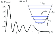
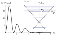
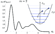
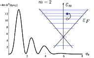
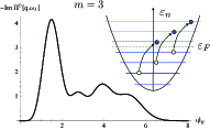
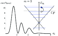
Figure 5: ${\rm Im}\,\Pi^{0}({\bf q},\omega_{m})$ for a 2DEG [plots (a), (c) and (e)] and for graphene [plots (b), (d) and (f)]. Here $\omega^{2DEG}_{m}=m\,\omega_{c}$ in a 2DEG and $\omega^{graph}_{m}=v_{\rm F}l_{B}^{-1}(\sqrt{2(N_{F}+m)}-\sqrt{2N_{F}})$ in graphene. The inset of each figure represents the different particle-hole excitations contributing at that energy. As we use $N_{F}=3$ for all the plots, there are $N_{F}+1=4$ maxima in ${\rm Im}\,\Pi^{0}({\bf q},\omega_{m})$ corresponding to islands (see text). Notice that for graphene, we show the polarizability at the energy of the first, second and fourth horizontal line of Fig. 4. The third line at this filling corresponds to the $(N_{F}+1,N_{F}-1)$ electron-hole pair and presents therefore $N_{F}$ peaks.

The presence of a set of islands – which is the name we give to regions of high spectral weight within each electron-hole contribution $(n+m,n)$ to a given horizontal line $m$ – can be understood from the form of the wave functions of the electron and the hole forming the pair. In the symmetric gauge, the modulus $|\Psi_{n,\ell}(x,y)|$ of the LL wave-function is rotation-invariant, its shape being that of $n+1$ concentric and equidistant rings (of average radius $r_{\ell}\simeq\sqrt{2\ell}l_{B}$).Giuliani and Vignale (2005) Therefore, one expects that electron-hole excitations of momentum $q$ will be possible whenever there is a finite overlap of the particle and hole wave-functions, the guiding centers of which are separated by a distance $\Delta R=l_{B}^{2}q$. If $n^{\prime}$ is the LL index of the electron and $n$ that of the hole, there are $n+1$ substantial overlaps of the rings of the electron and the hole wave functions when $\eta_{c}^{\prime}-\eta_{c}\leq\Delta R\leq\eta_{c}^{\prime}+\eta_{c}$. This will lead to a division of the contribution $(n^{\prime},n)$ to the $m$-th horizontal line of the PHES into $n+1$ regions of preferred momenta or islands.

In order to understand the effect of these overlap functions in more detail, we first consider the line $m=1$ of lowest energy. Both in the 2DEG and in graphene, the only possible inter-LL excitation that contributes to the formation of this energy line involves a hole in the LL $N_{F}$ and an electron in $N_{F}+1$. This is schematically represented in the inset of Fig. 5-(b), where we represent the unique electron-hole transition contributing to the first horizontal line in each case. As argued above, there are $N_{F}+1$ zones of preferred momenta due to the overlap between the wave functions of the electron and the hole. In Fig. 5(a) and (b), we have plotted ${\rm Im}\,\Pi^{0}({\bf q},\omega_{m})$ for the 2DEG and graphene, respectively, at the energy corresponding to the first horizontal line, with $N_{F}=3$. One obtains indeed four peaks which yield the islands observed in the low-energy zoom of the PHES (see Fig. 4 where we have also chosen $N_{F}=3$). Notice, however, that the last island, though present, is hardly visible in graphene due to the suppression of backscattering.

At larger values of $m$, there is an essential difference between the 2DEG and graphene. Due to the equidistant level spacing in LL quantization for non-relativistic electrons in the 2DEG, the horizontal lines in the PHES occur at $\omega_{m}=m\omega_{c}$. If $m>1$, there are $\min(m,N_{F})$ different inter-LL transitions $(n+m,n)$ that contribute to the spectral weight of the $m$-th horizontal line [see the inset of Fig. 5 and (e) which indicates the electron-hole transitions contributing to the second and third horizontal line in a 2DEG]. But all these transitions have different preferred momenta because of different electron-hole overlaps. The spectral weight is therefore a superposition of these different overlap functions [see Fig. 5(c), (e), where we plot ${\rm Im}\,\Pi^{0}({\bf q},\omega_{m})$ for $m=2,\,3$] and the islands are no longer well defined in the horizontal direction, as it may be seen in the second and third horizontal line of Fig. 4, which have lost the dashed structure of the first line. The situation is remarkably different in graphene, where the LL spacing is not constant and where a particular horizontal line is due to the inter-LL transition with energy $\omega_{n,m}^{\lambda}=\sqrt{2}(v_{\rm F}/l_{B})(\sqrt{n+m}-\lambda\sqrt{n})$ and therefore not only determined by the LL-index separation $m$. Apart from very rare events in the high-energy regime where two inter-LL transitions $(n_{1}+m_{1},n_{1})$ and $(n_{2}+m_{2},n_{2})$ may coincide in energy $\omega_{n_{1},m_{1}}^{\lambda}=\omega_{n_{2},m_{2}}^{\lambda^{\prime}}$, each horizontal line therefore consists of a single inter-LL transition and has $N_{F}+1$ well-separated peaks in ${\rm Im}\,\Pi^{0}({\bf q},\omega_{n,m}^{\lambda})$, as we have shown in Fig. 5(d), (f) for $(N_{F}+m,m)$, with $m=2,3$. In contrast to the 2DEG, the islands remain thus well separated in the horizontal direction, whereas they overlap strongly in the vertical direction (i.e. in energy) due to the decreasing level spacing at higher energies and the large number of inter-LL transitions in a fixed energy window [Fig. 4], as we have discussed in the last section. As a consequence, the most prominent modes in graphene in a strong magnetic field are diagonal lines, parallel to $\omega=v_{\rm F}q$, whereas those in the 2DEG remain horizontal. Electron-electron interactions turn these lines of large spectral weight into coherent modes: magneto-excitons in the 2DEG and linear magneto-plasmons in the case of graphene, in addition to the upper hybrid mode that reveals itself in the formerly forbidden energy region of the PHES of non-interacting particles.

VI Static screening

In this section we study the properties of $\Pi^{0}({\bf q})=\Pi^{0}({\bf q},\omega=0)$ in the static limit, for which the polarization is entirely real. The polarizability of graphene is shown in Fig. 6(a) and (b) for $B=0$Shung (1986); Wunsch et al. (2006); Hwang and Sarma (2007) and $B\neq 0$, respectively. For comparison, we also show the corresponding polarizability of a standard 2DEG Giuliani and Vignale (2005) in the absence [Figs. 6] and in the presence [Fig. 6] of a magnetic field. In order to compare the $B\neq 0$ to the $B=0$ polarizability, we have chosen a Fermi wave-vector $k_{F}$ for the $B=0$ case equal to $\sqrt{2N_{F}+1}/l_{B}$, which corresponds to the same carrier density as a graphene layer in a magnetic field with all LLs filled up to the $N_{F}$-th level of the conduction band.

One first notices a difference in the $B=0$ static polarizabilities between graphene and the 2DEG. Although the static polarizability remains constant and equal to the electronic density of states $\rho(\epsilon_{F})$, in both cases up to a wave vector $2k_{F}$, there are two contributions for graphene that stem from intra-band and inter-band excitations, respectively. Whereas the polarizability due to intra-band excitations in graphene [red dotted line in Fig. 6(a)] decreases linearly in $q$, due to the electrons’ chirality (17) and the absence of backscattering, the intra-band contributions yield a linearly increasing polarizability. Beyond $q=2k_{F}$, there are no possible zero-energy particle-hole excitations in the intra-band region, and the associated polarizability therefore tends to zero. This is also the case in the 2DEG [Fig. 6], where there are only intra-band excitations. In graphene, however, inter-band excitations still yield a linearly increasing contribution to the total polarizability, which then asymptotically approaches the inter-band polarizability [blue dashed line in Fig. 6(a)].

Qualitatively, one finds a similar behavior for the static polarizability at $B\neq 0$ except in the small-$q$ limit. Whereas the static polarizability at $B=0$ remains constant and coincides with the density of states at the Fermi energy, it tends to zero as $\Pi^{0}({\bf q}\rightarrow 0)\propto q^{2}$ for $B\neq 0$.Giuliani and Vignale (2005) This is due to the fact that the main contribution to the polarizability comes from ${\bf q}=0$ excitations in the vicinity of the Fermi energy $\epsilon_{F}$. Contrary to the $B=0$ case, where there are ${\bf q}=0$ excitations the energy of which tends to zero, $\epsilon_{F}$ lies now in the cyclotron gap between the highest occupied LL $N_{F}$ and the lowest unoccupied one $N_{F}+1$. This energy gap must be overcome by ${\bf q}=0$ excitations, such that its spectral weight tends to zero then. Indeed, the static polarizability also coincides with the density of states at the Fermi energy because the latter vanishes for $B\neq 0$ when $\epsilon_{F}$ lies in the gap.

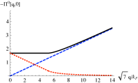
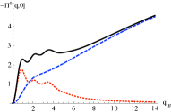
Figure 6: (Color online) (a) Vacuum (inter-band) contribution (blue dashed line), intra-band contribution (red dotted line) and total static polarization function (black thick line) of graphene for $B=0$ (see Ref.Hwang and Sarma, 2007). (b) Same as (a) but for $B\neq 0$. We have used $N_{F}=3$ and $N_{c}=350$. For consistency, the Fermi momentum used in (a) is $k_{F}=\sqrt{2N_{F}+1}/l_{B}=\sqrt{7}/l_{B}$. (c)-(d) Same as (a)-(b) respectively, but for a standard 2DEG.

Furthermore, one notices the oscillatory behavior of the static polarizability, both for graphene and the 2DEG, below $2k_{F}$. These oscillations are again due to the wave-function overlap between the electron and the hole, and one obtains $N_{F}+1$ maxima. Since the main contribution to the polarizability at small wave vectors comes from excitations in the vicinity of $\epsilon_{F}$, the oscillations are dominated by the $(N_{F}+1,N_{F})$ intra-band transition in graphene, as one may also see from the red dotted line in Fig. 6(b), which represents the intra-band contribution to the polarizability. At large values of the wave vector ${\bf q}$ the static polarizability is, as in the $B=0$ case, dominated by inter-band excitations the discrete nature of which is less important than in the small-${\bf q}$ limit. The linear increase therefore coincides with the $B=0$ result.

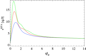
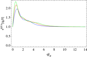
Figure 7: Static ($\omega=0$) dielectric function for graphene (a) and a 2DEG (b) in a magnetic field computed in the RPA. We have used $N_{F}=1,2,3$, corresponding to the blue, red and green lines, respectively.

The static polarizability is a useful quantity for the calculation of the screening properties of electrons. Screening, e.g. of the Coulomb interaction potential between the electrons or the potential of a charged impurity, is indeed determined by the (static) dielectric function $\varepsilon^{RPA}(q,\omega=0)=1-v(q)\Pi^{0}(q)$. At zero field, the long wavelength limit is similar in the two cases: $\varepsilon^{RPA}(q)\approx 1+q_{TF}/q$, where $q_{TF}\equiv 2\pi e^{2}\rho(\epsilon_{F})/\varepsilon_{b}$ is the Thomas-Fermi wave-vector. Note however that $q_{TF}$ is density independent in the 2DEG whereas it scales as $k_{F}$ in graphene. Therefore, the dielectric function diverges as $\varepsilon\sim q_{TF}/q\rightarrow\infty$ in the two cases when $q\to 0$. However, the $k_{F}$ dependence in the numerator of $\varepsilon^{RPA}(q\rightarrow 0)$ in graphene points out the absence of screening in undoped graphene $(k_{F}=0)$ at long distances. In the short wavelength region $q\gg 2k_{F}$, $\varepsilon^{RPA}(q)$ tends to 1 in a 2DEG, whereas for graphene, $\varepsilon^{RPA}(q)\rightarrow 1+\pi r_{s}/2$. This extra contribution of $\pi r_{s}/2$ to the dielectric function of graphene at large wave vectors is due to the linear growth of the polarizability at $q>2k_{F}$ and is therefore related to virtual inter-band particle-hole excitations.Ando (2006a) In summary, at short wavelengths, a 2DEG does not screen at all ($\varepsilon\to 1$), whereas (doped or undoped) graphene screens as a dielectric ($\varepsilon\to 1+\pi r_{s}/2>1$) thanks to its filled valence band.

The situation is different in the presence of a magnetic field. In Fig. 7(a) and (b) we have plotted the static dielectric function for graphene and the 2DEG, respectively, in a magnetic field (see also Ref. Shizuya, 2007, 2008). Notice that at long wavelengths, $\varepsilon^{RPA}(q)-1\propto q$ in the 2DEGAleiner and Glazman (1995) as well as in graphene. In fact, in the limit of $N_{F}\gg 1$,

$$\varepsilon^{RPA}(q)-1\propto r_{s}N_{F}^{3/2}ql_{B}$$ (20)

as $q\rightarrow 0$, this limit being valid for both, a 2DEG and graphene. The difference stems again in the density dependence of $r_{s}$ in the two cases: because $r_{s}\sim N_{F}^{-1/2}$ in a 2DEG, $\varepsilon^{RPA}$ grows linearly with $N_{F}$ in this case. However, $r_{s}$ is density-independent in graphene, leading to a dielectric function proportional to $N_{F}^{3/2}$. Furthermore the maximum of the dielectric function behaves as $\varepsilon_{\max}\simeq\varepsilon^{RPA}(q\sim 1/k_{F}l_{B}^{2})\sim r_{s}N_{F}$. Therefore $\varepsilon_{\max}\propto\sqrt{N_{F}}$ in a 2DEG whereas $\varepsilon_{\max}\propto N_{F}$ in graphene. This different behavior is reflected in Fig. 7 and (b). As we see, there is a considerable increase of the static dielectric function of graphene as we increase $N_{F}$, as compared to the 2DEG. This is due to the relativistic LL quantization of graphene, which leads to an increasing of the quantum effects (virtual inter-level transitions) as the separation between levels becomes narrower. On the other hand, in both graphene and the 2DEG, $\varepsilon^{RPA}(q,\omega=0)\rightarrow 1$ as $q\rightarrow 0$, which implies that there is no screening at long distances (as in the undoped zero field case, as discussed above). The short wavelength behavior of the dielectric function in a magnetic field is, however, similar in both the 2DEG and graphene to their respective zero field limits. Therefore, the short wavelength decay of the effective interaction in graphene, due to inter-band polarization effects, leads to a screening similar to that of an insulator, while the intra-band processes leads to a metallic-like screening.

VII Conclusions and Outlook

In conclusion, we have compared in detail the polarizability of doped graphene with and without a strong magnetic field to that of the 2DEG. In the absence of a magnetic field, the main difference arises from the presence of two different regions of non-vanishing spectral weight in the PHES ${\rm Im}\,\Pi({\bf q},\omega)$ of graphene. These two regions represent contributions from intra- and inter-band excitations, respectively, whereas in the 2DEG with only one parabolic band, there is only one region. Furthermore, the chirality of electrons in graphene suppresses backscattering such that the spectral weight is centered around the main diagonal of the PHES at $\omega=v_{\rm F}q$, whereas it is more or less homogeneously distributed over the particle-hole continuum in the 2DEG. Electron-electron interactions yield in both cases a plasmon mode that disperses as $\sqrt{q}$.

In the presence of a strong magnetic field, the plasmon mode evolves into the upper hybrid mode which is gapped at zero energy. In the 2DEG, this gap is given by the cyclotron frequency $\omega_{c}$, whereas in graphene it is $eBv_{\rm F}^{2}/\epsilon_{F}$ and thus depends on the Fermi energy $\epsilon_{F}$. The most salient difference between graphene and the 2DEG are the additional modes that occur in the interacting system in the parts of the PHES that correspond to the zero-field particle-hole continuum. In the 2DEG, the spectral weight is concentrated along equidistant horizontal lines, due to the equidistant LL spacing, and the resulting magneto-excitons are therefore weakly dispersing. In contrast to these rather well studied modes in the 2DEG, one finds linear magneto-plasmons in graphene that disperse roughly parallel to the central diagonal $\omega=v_{\rm F}q$ in the PHES. These modes are a consequence of a different organization of the regions of highest spectral weight in graphene as compared to the 2DEG. The energy levels in graphene are no longer equally spaced as a consequence of relativistic LL quantization, and the energies of inter-LL transitions are more densely packed than in the 2DEG, especially at higher energies. Even a small level broadening due to impurities therefore leads to an overlap in energy of the inter-LL transitions. Furthermore, spectral weight is highly modulated at a fixed energy due to the wave-function overlap between the electron and the hole involved in the excitation.

We have finally discussed the static polarizability and the dielectric function that describe the screening properties of the system. In contrast to the 2DEG, where the polarizability tends to zero at wave vectors larger than $2k_{F}$, it increases linearly in graphene, due to the increasing relevance of inter-band excitations. Whereas the small-$q$ behavior of the dielectric constant is similar in graphene and the 2DEG, a calculation within the RPA indicates that it tends to a constant different from one in the large-$q$ limit for graphene.

As for an experimental confirmation of the particular high-field collective excitations in graphene discussed above, one may first think of magneto-optical experiments. Transmission spectroscopy has indeed revealed the characteristic $\sqrt{Bn}$ behavior of the graphene LLs in epitaxial Sadowski et al. (2006) and exfoliated graphene,Jiang et al. (2007) in agreement with theoretical expecations.Gusynin et al. (2006); Gusynin and Sharapov (2006); Abergel and Fal ko (2007) Similarly, Raman spectroscopy has been successfully applied to graphene in the absence Yan et al. (2007); Pisana et al. (2007) and in the presence of a magnetic field.Faugeras et al. (2009) Thus the particular electron-phonon interaction Ando (2006b); Neto and Guinea (2007) and the theoretically studied magneto-phonon resonanceAndo (2007); Goerbig et al. (2007); Kashuba and Fal’ko (2009) could be confirmed. However, these techniques are restricted to zero wave-vector excitations, whereas electron-electron interactions and the resulting collective excitations are more prominent at non-zero values of the wave vector. In order to probe the excitation spectrum at non-zero values of the wave vector, inelastic light scattering may be a promissing technique that has been successfully used to study collective quantum-Hall excitations in the 2DEG.Eriksson et al. (1999); (43) (Ed.)

Appendix A Calculation of the polarization function

The electronic wave function in graphene in a magnetic field can be expressed as a four component spinor,

$$\Psi_{+}({\bf r},t)=e^{i{\bf K}\cdot{\bf r}}\left(\begin{array}[]{c}\Phi_{+A}({\bf r},t)\\ \Phi_{+B}({\bf r},t)\\ 0\\ 0\\ \end{array}\right)$$ (21)

$$\Psi_{-}({\bf r},t)=e^{-i{\bf K}\cdot{\bf r}}\left(\begin{array}[]{c}0\\ 0\\ \Phi_{-A}({\bf r},t)\\ \Phi_{-B}({\bf r},t)\\ \end{array}\right)$$ (22)

with the components

$$\Phi_{\zeta\alpha}({\bf r},t)=\sum_{\lambda=\pm}\sum_{n,\ell}\langle{\bf r}|\psi_{\zeta\alpha;\lambda n\ell}\rangle c_{\zeta;\lambda n\ell}(t)$$ (23)

where $c_{\zeta;\lambda n\ell}(t)$ is the annihilation operator of an electron in the state $|n,\ell\rangle$ of the $\lambda$ band with valley index $\zeta$. The ${\rm K}$ valley ($\zeta=+$) part of the single particle Green’s function in reciprocal space can be written as

$$G^{0}_{+}({\bf q},\omega)=\left(\begin{array}[]{cc}G^{0}_{+,AA}({\bf q},\omega)&G^{0}_{+,AB}({\bf q},\omega)\\ G^{0}_{+,BA}({\bf q},\omega)&G^{0}_{+,BB}({\bf q},\omega)\\ \end{array}\right),$$ (24)

with matrix elements

$$G_{\zeta;\alpha\alpha^{\prime}}^{0}({\bf k},\omega)=\sum_{\lambda}\sum_{n}\frac{f_{\zeta,\alpha\alpha^{\prime};\lambda n}({\bf k}+\zeta{\bf K})}{\omega-\lambda\xi_{n}+i\delta{\rm sgn}(\lambda\xi_{n})},\\$$ (25)

where $\lambda\xi_{n}=\lambda\epsilon_{n}-\epsilon_{F}$ is the energy difference between the LL and the Fermi energy $\epsilon_{F}=\epsilon_{N_{F}}$, which we choose in the conduction band ($\lambda=+$). Furthermore, $\delta$ is a positive infinitesimal in the clean limit and the matrix $f_{\lambda n}({\bf q})$ has been derived in Ref. Roldán et al., 2009. The expression for the Green’s function in the $K^{\prime}$ valley ($\zeta=-$) may be obtained with the help of $G_{\zeta;\alpha\alpha^{\prime}}^{0}=G_{-\zeta;\alpha^{\prime}\alpha}^{0}$, and the non-interacting polarization operator $\Pi^{0}({\bf q},\omega)$ can be calculated from Eq. (4). Taking into account both valleys, the particle-hole polarization reads

$$i\Pi^{0}({\bf q},\omega)=i\left[\Pi^{0}_{+}({\bf q},\omega)+\Pi^{0}_{-}({\bf q},\omega)\right]=2i\Pi^{0}_{+}({\bf q},\omega),$$ (26)

where the last step indicates that one obtains equal contributions from both valleys. We may therefore restrict the calculation to only one valley ($\zeta=+$), and take into account the twofold valley degeneracy by a simple factor $g_{v}=2$.

The integration over the frequency integral yields then Eq. (5), where the functions ${\cal\overline{F}}_{nn^{\prime}}^{\lambda\lambda^{\prime}}({\bf q})$ are given by

$${\cal\overline{F}}_{nn^{\prime}}^{\lambda\lambda^{\prime}}({\bf q})=\frac{e^{-l_{B}^{2}q^{2}/2}}{2\pi l_{B}^{2}}\left(\frac{l_{B}^{2}q^{2}}{2}\right)^{n_{>}-n_{<}}\left\{\lambda 1_{n}^{*}1_{n^{\prime}}^{*}\sqrt{\frac{(n_{<}-1)!}{(n_{>}-1)!}}\left[L_{n_{<}-1}^{n_{>}-n_{<}}\left(\frac{l_{B}^{2}q^{2}}{2}\right)\right]+\lambda^{\prime}2_{n}^{*}2_{n^{\prime}}^{*}\sqrt{\frac{n_{<}!}{n_{>}!}}\left[L_{n_{<}}^{n_{>}-n_{<}}\left(\frac{l_{B}^{2}q^{2}}{2}\right)\right]\right\}^{2}.$$ (27)

We defineRoldán et al. (2009)

$$\Pi_{+,nn^{\prime}}^{\,\,\,\lambda\lambda^{\prime}}({\bf q},\omega)=\frac{{\cal\overline{F}}_{nn^{\prime}}^{\lambda\lambda^{\prime}}({\bf q})}{\lambda\xi_{n}-\lambda^{\prime}\xi_{n^{\prime}}+\omega+i\delta}+(\omega^{+}\rightarrow-\omega^{-})$$ (28)

where $\omega^{+}\rightarrow\omega^{-}$ indicates the replacement $\omega+i\delta\rightarrow-\omega-i\delta$ and

$$\Pi_{+,n}^{\lambda}({\bf q},\omega) = \sum_{\lambda^{\prime}}\sum_{n^{\prime}=0}^{n-1}\Pi_{+,nn^{\prime}}^{\,\,\,\lambda\lambda^{\prime}}({\bf q},\omega)$$ (29)

$$+ \sum_{\lambda^{\prime}}\sum_{n^{\prime}=n+1}^{N_{c}}\Pi_{+,nn^{\prime}}^{\,\,\,\lambda\lambda^{\prime}}({\bf q},\omega)$$

$$+ \Pi_{+,nn}^{\lambda-\lambda}({\bf q},\omega)$$

which verify $\Pi_{+,n}^{\lambda}({\bf q},\omega)=-\Pi_{+,n}^{-\lambda}({\bf q},\omega)$. The vacuum polarization, which accounts for the inter-band processes, is defined as

$$\Pi^{vac}_{+}({\bf q},\omega)=-\sum_{n=1}^{N_{c}}\Pi_{+,n}^{\lambda=1}({\bf q},\omega)$$ (30)

where $N_{c}$ is a cutoff. Taking into account that, already in the absence of magnetic field, the validity of the continuum approximation is up to $\Lambda\sim t$, then $\epsilon_{N_{c}}=(v_{\rm F}/l_{B})\sqrt{2N_{c}}\sim t$, which leads to $N_{c}\sim 10^{4}/B[T]$, which is very high even for strong magnetic fields. However, due to the fact that the separation between LL in graphene decreases with $n$, it is always possible to have semiquantitative good results from smaller values of $N_{c}$.

Appendix B Electron-hole pair momentum

In this appendix, we relate the momentum ${\bf q}$ of an electron-hole pair to the distance between the guiding centers $\Delta{\bf R}$ of the electron and the hole. In classical mechanics, the cyclotron motion of an electron leads to ${\boldsymbol{\pi}}=e{\bf B}\times{\boldsymbol{\eta}}$, where ${\boldsymbol{\pi}}$ is the gauge-invariant momentum and ${\boldsymbol{\eta}}$ is the cyclotron coordinate. From Newton’s equation with Lorentz’s force, it is obvious that the quantity ${\bf K}\equiv{\boldsymbol{\pi}}-e{\bf B}\times{\bf r}$ is a constant of the motion, where ${\bf r}$ is the electron position. This constant of the motion is usually called the pseudo-momentum or generator of magnetic translations.Yoshioka (2002) Defining the guiding center coordinate as ${\bf R}={\bf r}-{\boldsymbol{\eta}}$, the pseudo-momentum reads ${\bf K}=e{\bf R}\times{\bf B}$, which actually shows that, apart from a conversion factor $eB=1/l_{B}^{2}$, the guiding center coordinate and the pseudo-momentum correspond to the same constant of the motion.

Now consider an electron-hole pair, where the electron has a pseudo-momentum ${\bf K^{\prime}}$ and the hole a pseudo-momentum $-{\bf K}$ (corresponding to a removed electron of pseudo-momentum ${\bf K}$). The pair has a momentum

$${\bf q}\equiv{\bf K^{\prime}}-{\bf K}=e\Delta{\bf R}\times{\bf B}$$ (31)

and therefore $\Delta R=ql_{B}^{2}$, which is the sought after relation.

References

- Ando et al. (1982) T. Ando, A. B. Fowler, and F. Stern, Rev. Mod. Phys. 54, 437 (1982).
- Neto et al. (2009) A. H. C. Neto, F. Guinea, N. M. R. Peres, K. S. Novoselov, and A. K. Geim, Rev. Mod. Phys. 81, 109 (2009).
- Iyengar et al. (2007) A. Iyengar, J. Wang, H. A. Fertig, and L. Brey, Phys. Rev. B 75, 125430 (2007).
- Shizuya (2007) K. Shizuya, Phys. Rev. B 75, 245417 (2007).
- Bychkov and Martinez (2008) Y. A. Bychkov and G. Martinez, Phys. Rev. B 77, 125417 (2008).
- Tahir and Sabeeh (2008) M. Tahir and K. Sabeeh, J. Phys.: Condens. Matter 20, 425202 (2008).
- Berman et al. (2008) O. L. Berman, G. Gumbs, and Y. E. Lozovik, Phys. Rev. B 78, 085401 (2008).
- Roldán et al. (2009) R. Roldán, J.-N. Fuchs, and M. O. Goerbig, Phys. Rev. B 80, 085408 (2009).
- Fischer et al. (2009) A. M. Fischer, A. B. Dzyubenko, and R. A. Romer (2009), eprint arXiv:0902.4176.
- Giuliani and Vignale (2005) G. F. Giuliani and G. Vignale, Quatum Theory of the Electron Liquid (Cambridge University Press, Cambridge, 2005).
- Kallin and Halperin (1984) C. Kallin and B. I. Halperin, Phys. Rev. B 30, 5655 (1984).
- Shung (1986) K. W. K. Shung, Phys. Rev. B 34, 979 (1986).
- Ando (2006a) T. Ando, J. Phys. Soc. Jpn. 75, 074716 (2006a).
- Wunsch et al. (2006) B. Wunsch, T. Stauber, F. Sols, and F. Guinea, New Journal of Physics 8, 318 (2006).
- Hwang and Sarma (2007) E. H. Hwang and S. D. Sarma, Phys. Rev. B 75, 205418 (2007).
- Shon and Ando (1998) N. H. Shon and T. Ando, J. Phys. Soc. Jpn. 67, 2421 (1998).
- Stern (1967) F. Stern, Phys. Rev. Lett. 18, 546 (1967).
- Czachor et al. (1982) A. Czachor, A. Holas, S. R. Sharma, and K. S. Singwi, Phys. Rev. B 25, 2144 (1982).
- Chiu and Quinn (1974) K. W. Chiu and J. J. Quinn, Phys. Rev. B 9, 4724 (1974).
- González et al. (1994) J. González, F. Guinea, and M. A. H. Vozmediano, Nucl. Phys. B 424, 595 (1994).
- Sabio et al. (2008) J. Sabio, J. Nilsson, and A. H. Castro-Neto, Phys. Rev. B 78, 075410 (2008).
- Katsnelson (2006) M. I. Katsnelson, Phys. Rev. B 74, 201401 (2006).
- Gangadharaiah et al. (2008) S. Gangadharaiah, A. M. Farid, and E. G. Mishchenko, Physical Review Letters 100, 166802 (2008).
- Polini et al. (2008) M. Polini, R. Asgari, G. Borghi, Y. Barlas, T. Pereg-Barnea, and A. H. MacDonald, Phys. Rev. B 77, 081411 (2008).
- Polini et al. (2009) M. Polini, A. H. MacDonald, and G. Vignale (2009), eprint arXiv:0901.4528.
- Shizuya (2008) K. Shizuya, Phys. Rev. B 77, 075419 (2008).
- Aleiner and Glazman (1995) I. L. Aleiner and L. I. Glazman, Phys. Rev. B 52, 11296 (1995).
- Sadowski et al. (2006) M. L. Sadowski, G. Martinez, M. Potemski, C. Berger, and W. A. de Heer, Phys. Rev. Lett. 97, 266405 (2006).
- Jiang et al. (2007) Z. Jiang, E. A. Henriksen, Y.-J. W. L. C. Tung, M. E. Schwartz, M. Y. Han, P. Kim, and H. L. Stormer, Phys. Rev. Lett. 98, 197403 (2007).
- Gusynin et al. (2006) V. P. Gusynin, S. G. Sharapov, and J. P. Carbotte, Phys. Rev. Lett. 96, 256802 (2006).
- Gusynin and Sharapov (2006) V. P. Gusynin and S. G. Sharapov, Phys. Rev. B 73, 245411 (2006).
- Abergel and Fal ko (2007) D. Abergel and V. I. Fal ko, Phys. Rev. B 75 75, 155430 (2007).
- Yan et al. (2007) J. Yan, Y. Zhang, P. Kim, and A. Pinczuk, Phys. Rev. Lett. 98, 166802 (2007).
- Pisana et al. (2007) S. Pisana, M. Lazzeri, C. Casiraghi, K. S. Novoselov, A. K. Geim, A. C. Ferrari, and F. Mauri, Nature Mat. 6, 198 (2007).
- Faugeras et al. (2009) C. Faugeras, M. Amado, P. Kossacki, M. Orlita, M. Sprinkle, C. Berger, W. de Heer, and M. Potemski, arXiv:0907.5498 (2009).
- Ando (2006b) T. Ando, J. Phys. Soc. Jpn. 75, 124701 (2006b).
- Neto and Guinea (2007) A. C. Neto and F. Guinea, Phys. Rev. B 75, 045404 (2007).
- Ando (2007) T. Ando, J. Phys. Soc. Jpn. 76, 024712 (2007).
- Goerbig et al. (2007) M. O. Goerbig, J.-N. Fuchs, V. I. Fal’ko, and K. Kechedzhi, Phys. Rev. Lett. 99, 087402 (2007).
- Kashuba and Fal’ko (2009) O. Kashuba and V. I. Fal’ko, arXiv:0906.5251 (2009).
-
Das Sarma and Pinzcuk (1997)pinczuk
S. Das Sarma and
A. Pinzcuk (Ed.),
Perspectives in Quantum Hall Effects
(John Wiley, New York, 1997).
- Eriksson et al. (1999) M. A. Eriksson, A. Pinczuk, B. S. Dennis, S. H. Simon, L. N. Pfeiffer, and K. W. West, Phys. Rev. Lett. 82, 2163 (1999).
missing- Yoshioka (2002) D. Yoshioka, The Quantum Hall Effect (Springer-Verlag Berlin Heidelberg, 2002).
- Eriksson et al. (1999) M. A. Eriksson, A. Pinczuk, B. S. Dennis, S. H. Simon, L. N. Pfeiffer, and K. W. West, Phys. Rev. Lett. 82, 2163 (1999).