HAWC Timing Calibration

Abstract

The High-Altitude Water Cherenkov (HAWC) Experiment is a second-generation high-sensitivity gamma-ray and cosmic-ray detector that builds on the experience and technology of the Milagro observatory. Like Milagro, HAWC utilizes the water Cherenkov technique to measure extensive air showers. Instead of a pond filled with water (as in Milagro) an array of closely packed water tanks is used. The event direction will be reconstructed using the times when the PMTs in each tank are triggered. Therefore, the timing calibration will be crucial for reaching an angular resolution as low as 0.25 degrees. We propose to use a laser calibration system, patterned after the calibration system in Milagro[1]. Like Milagro, the HAWC optical calibration system will use $\sim$1 ns laser light pulses. Unlike Milagro, the PMTs are optically isolated and require their own optical fiber calibration. For HAWC the laser light pulses will be directed through a series of optical fan-outs and fibers to illuminate the PMTs in approximately one half of the tanks on any given pulse. Time slewing corrections will be made using neutral-density filters to control the light intensity over 4 orders of magnitude. This system is envisioned to run continuously at a low rate and will be controlled remotely. In this paper, we present the design of the calibration system and first measurements of its performance.

Gamma rays, cosmic rays, water Cherenkov

1 Introduction

The High-Altitude Water Cherenkov (HAWC) Experiment will be built at 4100 meters on a plateau below the highest mountain in Mexico, the Pico de Orizaba. It will be 10 to 15 times more sensitive than its predecessor, the Milagro Observatory[2]. Like Milagro, HAWC will survey the sky (from its location at 19^o north latitude) continuously measuring extensive air showers generated by cosmic and gamma rays, leading to a large field-of-view of $\sim$2 sr. The physics goal of HAWC is to make major progress in studying the origin of of cosmic rays. This can be achieved by detecting the highest energy gamma-ray sources ($\sim$100 TEV) and by measuring and mapping the galactic diffuse gamma-ray emission from 1 TeV to 100 TeV. Because of its $\sim 100$% duty cycle, HAWC is particularly well suited to search for transients, new galactic and extragalactic sources of VHE gamma-radiation, and for small- and large-scale anisotropies in the cosmic radiation in an unbiased sky survey. In order to meet these physics goals, good angular resolution is essential. With HAWC we aim for an angular resolution between 0.25^∘ and 0.55^∘, where 0.55^∘ is representative of low energies and 0.25^∘ of high energies. As in Milagro the shower direction will be reconstructed using the relative times at which each of the PMTs is hit. In this paper, we will describe the design of the optical calibration system that will be used to monitor the relative time responses of each PMT in the HAWC detector.

2 The HAWC Detector

The HAWC Observatory is described in more detail elsewhere in these Proceedings [3]. It will re-use the 900 8” PMTs[4] from Milagro. The PMTs will be deployed at a depth of $\sim$4 m of water in separate tanks. The tanks will be closely packed in an array covering an area of approximately 150m x 150m. Depending on the detailed design, more than 60% of this area will be covered with water. Two alternative designs are under consideration: one with 900 individual rotomolded water tanks of $\sim 4$m diameter holding one PMT; a second with 7.3m diameter tanks (which are a combination of corrugated galvanized steel walls and a water-tight bladder) holding three PMTs. Each tank will have one or more 8” baffled, upward-facing PMT(s) anchored to the bottom. Figure 1 shows a sketch of the proposed 900 tank deployment pattern.

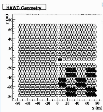
Figure 1: A sketch of one proposed layouts for the tanks of the HAWC detector. The rectangle in the center represents the counting house; this is also the site of the calibration light sources. The black and white pattern of the tanks (in the lower-right of the figure) is explained in the text.

3 The Calibration System

The primary goal of the optical calibration system is to monitor the time stability of the PMTs and related readout/digitization electronics. To achieve an angular resolution of $<$0.55^∘ it is not only necessary to know the position of each PMT to only a few cm, but also to know the relative times at which each PMT in the array has been hit to an uncertainty of $\leq 1$ns. Furthermore the channel to channel timing drifts and the slewing must be monitored and corrected for accordingly[5]. The components of the HAWC optical calibration system are chosen to meet this goal. This includes e.g. the $<1$ns pulse-width laser light source[6] and the use of equal length, duplex optical fibers on all fiber paths. Furthermore to monitor the time slewing and to measure the photo-electron calibration of each (PMT) channel[5], filter wheels at the laser light source will allow control of the light pulses over a dynamic range from $\sim 0.1$ PE to $>1000$ PEs.

For reasons of practicality and redundancy, the tank PMTs are divided into two groups: denoted black and white for optical calibration. This is sketched in Figure 1 where $\sim 16$ physically nearby PMTs form a black (or white) square. The pattern of squares is similar to the pattern on a checker(chess) board. A possible pattern of squares is shown (for the lower-right quadrant of the array) in Figure 1. The calibration design foresees two separate laser light delivery systems. One laser plus optical distribution system will be used to pulse all of the black tanks, a second system will pulse all of the white tanks. The two laser systems and associating monitoring instrumentation will be located in a temperature controlled enclosure at the center of the HAWC array (shown as black rectangle in the center of the array in Figure 1).

Figure 2 shows a sketch of one of the proposed light sources and its associating instrumentation. The light from the Teem Photonics PowerChip laser[6] will be sent through a beam expander[7] into a 1:37 optical splitter[8] at the calibration light source. The 1:37 optical splitter will fan-out the laser light pulses into the ${}^{>}_{\sim}$ 30 paths leading to the centers of all black (or white) squares of tanks. To connect to the approximate center of each square we will use same-length, $\sim$200m long, $62.5\mu$m/125 $\mu$m graded index duplex fibers. Finally at each square the light is split again to be routed on $\sim$25m fibers to each tank (see Figure 3) where the fibers will be terminated with a simple diffuser positioned at a fixed distance from each tank PMT. Additionally there will be one loop-back duplex fiber for monitoring (double) the optical fiber light transmission time for a representative light path for each square, and $\sim 1$ fiber to a tank in the adjacent square to link the timing of black and white optical calibrations.

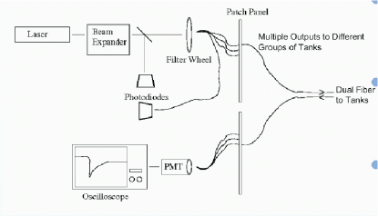
Figure 2: Sketch of one of two HAWC light sources for the optical timing calibration system. The light sources will be located at the center of the array; see Figure 1. See text for details.

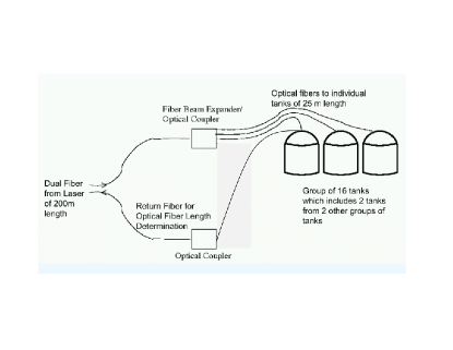
Figure 3: Sketch of one of approximately 60 HAWC field distributions of the laser light for the optical timing calibration system. Each of the field distributions will be located near the center of the black (or white) squares. The field distributions further split the laser light pulses to the fibers that then go to each PMT. Additionally one duplex fiber (per square) will be run to one (representative) tank and the signal looped-back to be monitored for end-to-end timing at the light source; see Figure 2.

The $\sim$200m long, duplex fibers naturally provide an outgoing and a return light path. The outgoing light path is needed to deliver the laser light pulses to the center of each square. The return light path is used to monitor the light pulses by returning one representative signal; see Figure 3. In summary the outgoing light follows the path from: the laser, into the 1:37 splitter, coupled through a patch panel (at the light source see Figure 2), into the $\sim$200m long fiber to the field distribution at the center of each square where the light is split again to be routed on $\sim$25m fibers to each tank. The return light path will be exactly double the total optical fiber light path and is used to return a representative light signal from each square; see Figure 3. Again for both redundancy and practicality reasons, the return light pulses are merged using four 19:1 optical fan-ins[8], one for each quadrant of the array; see Figure 2. The return light will then be monitored with a small photo-tube[9]. Up to small timing differences, all return signals will arrive at the same time. Thus to distinguish each light path, we are considering adding optical delay fibers, in increments of $\sim 5$m of fiber delay, between the return light fibers from the squares and the 1:19 optical fan-ins. In this way each light path can be easily monitored. An example, showing the return light from three separate calibration loop-back signals, is shown in Figure 4. The relative time delay from 5m optical fiber is 25.6ns.

Assuming a relative timing delay of $\geq$5m of optical fiber, the distinct light signals observed in the initial proof of principle study (Figure 4) suggests that it should be straight forward to monitor all light paths to a precision of $\sim 1$ns using e.g. a 4-channel digital oscilloscope digitize the return light pulses for each of the optical calibration light paths.

4 Tests of the Calibration System

Several laboratory tests of the calibration system have already been performed. These have focused on proof of principle tests: e.g. how uniform are the light signals in the 37 output fibers of the 1:37 optical splitter at the light source, or the light signals in the 19 optical fibers of the 1:19 optical splitter at the field distribution at each square. The other critical issue is the expected light at the individual tank PMTs and whether it can result in $>1000$ PEs (the maximum signal needed to monitor the PMT/readout time slewing corrections).

To achieve uniform fiber-to-fiber illumination with any 1:n splitter requires that the size of the light spot is significantly larger than the size of the fiber bundle. Laser beams can be increased in size easily using commercial beam expanders. The balance is then between fiber-to-fiber uniformity and the signal size in each fiber: more uniformity comes at the cost of decreased signal size. First measurements with the JDS Uniphase Power Chip laser[1] find that expanding the beam at the laser by a factor of $\sim 5\times$ results in a rather uniform illumination of the 1:37 optical fiber splitter[8]. A LaserProbe RM6600A radiometer with a RjP-465 silicon sensor[10] has been used to measure the laser intensity and the signals into the optical fibers. As an example, with a $5\times$ beam expander. typical fiber signals were $\sim 15$nJ ($\pm$25%) per pulse, while the measured laser energy was $\sim 22\mu$J.

In tests of the field distribution, an aspheric lens with a focal length of 4.5mm[11] was used to create a collimated beam from the light source fiber into the 1:19 optical splitter. However it was found that the (light source) fiber speckle pattern resulted in a non-uniform light intensity within the collimated beam. One solution was to add a simple ground glass diffuser[12] between the lens and the 1:19 splitter. While this decreased the the light intensity into the individual fibers of the 1:19 splitter, the net impact is on the design and positioning of the tank diffuser (next paragraph). An alternate possibility (yet to be studied) is to reduce the amount of speckle by randomizing the polarization of the laser light at the source.

The design of the tank light diffuser, mounted on the end of the optical fiber(s) in each tank, has not been finalized. However estimates of the light intensity at the HAWC tanks have been made by including all elements of the HAWC calibration up to (but not including) the final tank optical diffusers. The resulting table top mock-up of the HAWC calibration system included: the (existing) PowerChip laser, $5\times$ beam expander, 1:37 fiber splitter, 2 x 150m of $62.5\mu$m/$125\mu$m optical fiber distribution, and the field distribution optics (including the ground glass diffuser and 1:19 fiber splitter). Including a $\sim 8$% quantum efficiency for the 8” Hamamatsu PMTs[4] at the calibration wavelength of 532nm, we expect $>1000$ PEs in the PMTs as long as the light coupling efficiency is $>1$% between the calibration optical fiber (diffuser) and the 8” PMTs. This argues for mounting the tank optical diffusers close to the PMTs. This choice also minimizes possible PMT to PMT laser light time arrival differences from any light path length differences in the tanks.

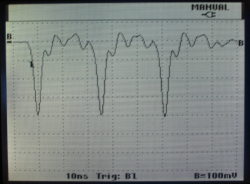
Figure 4: The observed return-light time distribution from three separate calibration light paths. The 200 Mhz oscilloscope has somewhat limited bandwidth for the fast $\sim 1$ns light pulses. The relative time delays between the three light paths is the result of the addition of 5m and 10m of (additional) optical fiber to two of the light paths. The near equality of the signals shows the good uniformity of the light coupling into the 1:37 output and 1:19 return optical fan-outs/fan-ins.

5 Conclusion

A table-top realization of the proposed HAWC optical calibration system was set up to evaluate in detail the timing calibration of the HAWC detector. The components of the calibration system have been tested for their performance, in particular their timing stability and the expected light intensity delivered to the individual tanks. No obstacles have been found. Future efforts will focus on optimizing the light yield (and fiber to fiber uniformity) as well as the design of the tank diffuser and tank diffuser mounting plan.

References

- [1] JDS Uniphase PowerChip NanoLaser with a measured energy of J/pulse at 532nm. This is somewhat less than the original vendor specified energy of J/pulse. This laser is now made by Teem Photonics[6] (below).
- [2] Atkins, R., et al., Astrophys. J., 608 680 (1999)
-
[3]
“HAWC in the Fermi Era”, J. Goodman, University of Maryland, for the HAWC collaboration
“The HAWC observatory and its synergies at volcan Sierra Negra”, H. Salazar for the HAWC collaboration