Deconfining phase transition on a double-layered torus

Abstract:

Deconfined regions in relativistic heavy ion collisions are limited to small volumes surrounded by a confined exterior. Here the geometry of a double layered torus is discussed, which allows for different temperatures in its two layers. This geometry enables one to approach the QCD continuum limit for small deconfined volumes with confined exteriors in a more realistic fashion than by using periodic boundary conditions. Preliminary data from a study for pure SU(3) lattice gauge theory support a substantial increase in a pseudo transition temperature.

1 Equilibrium simulations of the deconfinement transition and lab plasma

Statistical properties of a quantum system with Hamiltonian $H$ in a continuum volume $V$, which is in equilibrium with a heatbath at physical temperature $T$, are determined by the partition function

$$Z(T,V)={\rm Tr}e^{-H/T}=\sum_{\phi}\langle\phi|e^{-H/T}|\phi\rangle,$$ (1)

where the sum extends over all states and the Boltzmann constant is set to one. Imposing periodic boundary conditions (PBC) in Euclidean time $\tau$ and bounds of integration from $0$ to $1/T$, one can rewrite the partition function in the path integral representation:

$$Z(T,V)=\int D\phi\exp\left\{-\int_{0}^{1/T}d\tau L_{E}(\phi,\dot{\phi})\right\}.$$ (2)

Nothing in this formulation requires to carry out the infinite volume limit.

Past LGT simulations of the deconfining transition focused primarily on boundary conditions (BC), which are favorable for reaching the infinite volume quantum continuum limit (thermodynamic limit of the textbooks) quickly with temperature and volume of the system given by

$$T=\frac{1}{a\,N_{\tau}}=\frac{1}{L_{\tau}}\,,~{}~{}~{}N_{s}/N_{\tau}\to\infty\,,~{}~{}N_{\tau}\to\infty\,,~{}~{}L_{\tau}~{}{\rm finite}\,,$$ (3)

where $a$ is the lattice spacing. These are PBC in the spatial volume $V=(a\,N_{s})^{3}$. For the deconfinement phase created in a heavy ion collision the infinite volume limit does not apply. Instead we have to take the finite volume continuum limit

$$N_{s}/N_{\tau}={\rm finite}\,,~{}~{}N_{\tau}\to\infty\,,~{}~{}L_{\tau}~{}{\rm finite}\,,$$ (4)

and PBC are incorrect because the outside is in the confined phase at low temperature. E.g., at the BNL RHIC one expects to create an ensemble of differently shaped and sized deconfined volumes. The largest volumes are those encountered in central collisions. A rough estimate of their size is

$$\pi\times(0.6\times{\rm Au\ radius})^{2}\times c\times({\rm expansion\ time})$$ (5)

$$=(55\ {\rm fermi}^{2})\times({\rm a\ few\ fermi})$$

where $c$ is the speed of light. Here we want to estimate finite volume corrections for pure SU(3) and focus on the continuum limit for

$$L_{s}=aN_{s}=(5-10)\ {\rm fermi}\ .$$ (6)

In the following we set the physical scale by

$$T^{c}=174\ {\rm MeV}\ ,$$ (7)

which is in the range of QCD estimates with two light flavor quarks, implying for the temporal extension

$$L_{\tau}=a\,N_{\tau}=1.13\ {\rm fermi}\ .$$ (8)

2 Simulations with cold boundary conditions

We consider difficulties and effects encountered when one equilibrates a hot volume with cold boundaries by means of Monte Carlo (MC) simulations for which the updating process provides the equilibrium. We use the single plaquette Wilson action on a 4D hypercubic lattice. Numerical evidence shows that SU(3) lattice gauge theory exhibits a weakly first-order deconfining phase transition at some coupling $\beta^{g}_{t}(N_{\tau})=6/g^{2}_{t}(N_{\tau})$. The scaling behavior of the deconfining temperature is

$$T^{c}=c_{T}\,\Lambda_{L}$$ (9)

where the lambda lattice scale

$$a\,\Lambda_{L}=f_{\lambda}(\beta^{g})=\lambda(g^{2})\,\left(b_{0}\,g^{2}\right)^{-b_{1}/(2b_{0}^{2})}\,e^{-1/(2b_{0}\,g^{2})}\,,$$ (10)

has been determined in the literature. The coefficients $b_{0}$ and $b_{1}$ are perturbatively obtained from the renormalization group equation,

$$b_{0}=\frac{11}{3}\frac{3}{16\pi^{2}}~{}~{}{\rm and}~{}~{}b_{1}=\frac{34}{3}\left(\frac{3}{16\pi^{2}}\right)^{2}\,.$$ (11)

Higher perturbative and non-perturbative corrections are parametrized in [1] by

$$\lambda(g^{2})\ =\ 1+a_{1}\,e^{-a_{2}/g^{2}}+a_{3}\,g^{2}+a_{4}\,g^{4}~{}~{}~{}{\rm with}$$ (12)

$a_{1}=71553750,\ a_{2}=19.48099,\ a_{3}=-0.03772473,\ a_{4}=0.5089052.$ In the region accessible by MC simulations this parametrization is perfectly consistent with an independent earlier one in [2], but has the advantage to reduce for $g^{2}\to 0$ to the perturbative limit.

Imagine an almost infinite space volume $V=L_{s}^{3}$ and a smaller sub-volume $V_{1}=L_{s,1}^{3}.$ The complement to $V_{1}$ in $V$ will be called $V_{0}$ (outside world). The number of temporal lattice links $N_{\tau}$ is the same for both volumes. We like to find parameters so that scaling holds in both volumes, while $V_{1}$ is at temperature $T_{1}=T_{c}$ and $V_{0}$ at room temperature $T_{0}$. We denote the coupling by $\beta^{g}_{0}$ for plaquettes in $V_{0}$ and by $\beta^{g}_{1}$ for plaquettes in $V_{1}$. For that purpose any plaquette touching a site in $V_{1}$ is considered to be in $V_{1}$. We would like to have $\beta^{g}_{1}$ in the scaling region, say $\beta^{g}_{1}=6.$ The relation

$$10^{10}\approx\frac{T_{1}}{T_{0}}=\frac{a_{0}}{a_{1}}=\frac{f_{\lambda}(\beta_{0}^{g})\,\Lambda_{L}}{f_{\lambda}(\beta^{g}_{1})\,\Lambda_{L}}=\frac{f_{\lambda}(\beta_{0}^{g})}{f_{\lambda}(\beta^{g}_{1})}$$ (13)

drives $\beta^{g}_{0}$ out of the scaling region and (after moving over to strong coupling relations) practically to $\beta^{g}_{0}=0$, which we call disorder wall BC. In the disorder wall approximation of the cold exterior we can simply omit contributions from plaquettes that involve links through the boundary. MC simulations, which we quickly summarize here, were performed in Ref.[3]. Due to the use of the strong coupling limit for the outside volume, scaling of the results is not obvious.

We use the maxima of the Polyakov loop susceptibility

$$\chi_{\max}=\frac{1}{N_{s}^{3}}\left[\langle|P|^{2}\rangle-\langle|P|\rangle^{2}\right]_{\max},\,\,\,P=\sum_{\vec{x}}P_{\vec{x}}$$ (14)

to define pseudo-transition couplings $\beta^{g}_{pt}(N_{s};N_{\tau})$. Our BC introduce an order $N_{s}^{2}$ disturbance, so that

$$\beta^{g}_{pt}(N_{s};N_{\tau})=\beta^{g}_{t}(N_{\tau})+a_{1}^{d}\,\frac{N_{\tau}}{N_{s}}+a_{2}^{d}\,\left(\frac{N_{\tau}}{N_{s}}\right)^{2}+a_{3}^{d}\,\left(\frac{N_{\tau}}{N_{s}}\right)^{3}+\ \dots$$ (15)

holds.

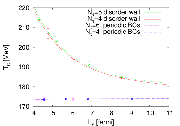
Figure 1: Estimates of finite volume corrections to $T_{c}$.

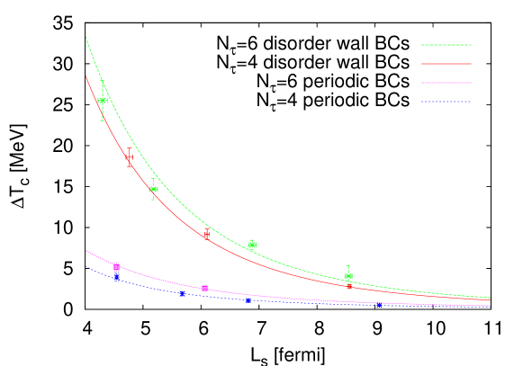
Figure 2: Estimates of finite volume corrections to the width of the Polyakov loop susceptibility.

Fits of pseudo-transition coupling constant values lead to estimates of finite volume corrections to $T_{c}$ as given in Fig. 1. It is seen from the figure that they are consistent with scaling as the curves for $N_{\tau}=4$ and $N_{\tau}=6$ fall on top of one another. There are no free parameters involved at this point, because the non-perturbative parametrization of the SU(3) lambda scale was determined in independent literature. Estimates of finite volume corrections to the full width of Polyakov loop susceptibilities at 2/3 maximum are shown in Fig. 2. Again, the curves are found to be consistent with scaling.

Results so far show that for volumes of BNL RHIC size the magnitudes of $T_{c}$ and width corrections are comparable to those obtained by including quarks into pure SU(3) calculations ($T_{c}$ in the opposite, width in the same direction). Similar corrections are expected for the equation of state. Previous QCD calculations at finite temperatures and densities should therefore be extended to cold BC.

However, there remain problematic questions about disorder wall BC. Although the results show scaling, it is unsatisfactory that the disorder wall BC do not reflect a physical outside volume. Two properties are desirable:

1. Inside and outside volumes are kept in the scaling region.

2. The spatial lattice spacing $a_{s}$ is the same on both sides of the boundary.

In such simulations one may again keep $T_{\rm inside}$ at $T_{c}$ and study its dependence on $T_{\rm outside}$. As outlined in the next section, this can be done in the newly introduced geometry [4] of a double layered torus (DLT), but has then to be done for a rather small $T_{\rm outside}$ interval

$$T_{\rm outside}\in\left[T_{c}-\triangle T,T_{c}\right]\,,~{}~{}\triangle T>0\,.$$ (16)

3 Simulations on a double layered torus

Figure 3: Double layered torus in two dimensions.

For the DLT the boundaries are glued together as indicated by the arrows in Fig. 3. Note that interchanging labels 3 and 4 on one of the lattices leads to a situation in which some sites are connected by two links and the different geometry of a sphere.

With DLT BC in the spacelike directions and PBC in the fourth direction one can simulate at two temperatures and each volume becomes the outside world of the other. The two temperatures are adjusted by tuning the coupling constants in the two volumes. MPI Fortran code for SU(3) simulations on a DLT is given in Ref.[4, 5]. Preliminary numerical results with both temperatures in the SU(3) scaling region are compiled in the following.

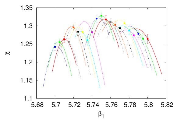
Figure 4: Polyakov loop susceptibilities on a $8^{3}4$ DLT.

Figure 4 shows the reweighting in $\beta_{1}$ of Polyakov loop susceptibilities on a $8^{3}4$ lattice, each simulation point corresponding to a different pair of coupling constant values $(\beta_{0}^{0},\beta_{1}^{0})$, adjusted so that $\beta_{1}^{0}$ is close to the pseudocritical point.

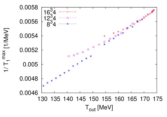
Figure 5: Inverse pseudo transition temperatures versus outside temperatures.

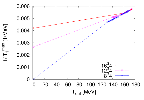
Figure 6: Results of the previous figure together with disorder wall estimates.

Using scaling relations the inverse physical pseudocritical temperatures, $1/T_{1}^{\max}$ from all our lattice sizes, with $T_{1}^{\max}$ corresponding to the maxima of the Polyakov loop susceptibilities, are plotted in Fig. 5 versus the outside temperature $T_{\rm out}$. Even for the small range of outside temperatures in the SU(3) scaling region, one sees already sizable corrections of $T_{1}^{\max}$. The same data are plotted in Fig. 6, extending the $T_{\rm out}$ down to zero, so that the estimates from Ref.[3] can be included (on the $8^{3}4$ lattice not transition was found with disorder wall BC as indicated here by $1/T_{1}^{\max}=0$).

In summary, our preliminary DLT results in the scaling region are consistent with the disorder wall finite volume $T_{c}$ estimates. These simulations keep inside and outside temperatures in the SU(3) scaling region. To achieve also a continuous spacelike lattice spacing across the boundary, one has to use asymmetric couplings in space and time directions. Considerable work remain to be done to obtain an overall convincing description.

Acknowledgments: This work has in part been supported by DOE grants DE-FG02-97ER-41022, DE-FC02-06ER-41439, by NSF grant 0555397, and by the German Humboldt Foundation. BB thanks Wolfhard Janke and his group for their kind hospitality at Leipzig University. Simulations were performed at NERSC under ERCAP 82860 and on PC clusters at FSU.

References

- [1] A. Bazavov, B.A. Berg, and A. Velytsky, Phys. Rev. D 74 (2006) 014501.
- [2] S. Necco and R. Sommer, Nucl. Phys. B 622 (2002) 328.
- [3] A. Bazavov and B.A. Berg, Phys. Rev. D 76 (2007) 014502.
- [4] B.A. Berg, arXiv:0904.0642.
- [5] B.A. Berg and H. Wu, arXiv:0904.1179.